ISTANBUL BILGI UNIVERSITY INSTITUTE OF GRADUATE PROGRAMS
FINANCIAL ECONOMICS MASTER’S DEGREE PROGRAM
MEASURING FINANCIAL STRESS INDEX FOR TURKEY
AYŞEGÜL KOYUNLU 116620008
Dr. Öğr. Üyesi SEMA BAYRAKTAR
ISTANBUL 2019
iii PREFACE
This study is submitted in fulfillment of the requirements of the Master’s Degree of Financial Economics program at Istanbul Bilgi University. The studies related to the measurement of financial stress index taking into account different market segments together has become important especially after the late 1990s. The previous studies were mostly focused on a single market and ignored the systemic impacts of it.
In this study, a financial stress index is constructed for Turkey by using a relatively new variable which is rarely used in the related literature. The objective is to predict the financial stress periods for Turkey by using different methods.
I would like to express my gratitude and thanks to my advisor Dr. Sema Bayraktar for her encouragement and invaluable support during my study. For his
encouragements and helps,I am also thankful to my brother Sercan Koyunlu.
Ayşegül Koyunlu Istanbul, May 2019
iv CONTENT PREFACE ... iii CONTENTS ... iv LIST OF ABBREVIATIONS ... iv LIST OF SYMBOLS ... vi
LIST OF FIGURES ... viii
LIST OF TABLES ...x ABSTRACT ... xi ÖZET... iv INTRODUCTION ...1 CHAPTER 1 LITERATURE REVIEW...4 CHAPTER 2 METHODOLOGY...15
2.1. Construction of a Composite Index of Financial Stress ... 15
2.1.1. Volatility Measures ...15
2.1.1.1. Generalized Autoregressive Conditional Heteroscedasticity Models ...16
2.1.1.1.1. GARCH (1, 1) Model...16
2.1.1.1.2. GJR – GARCH (1, 1) Model ...17
2.1.1.1.3. E - GARCH (1, 1) Model ...17
2.1.1.2. Volatility Measure for BIST100 Banking Sector Index ...19
2.1.1.3. Volatility Measure For Currency Basket Indicator ...20
2.1.1.4. Volatility Measure For BIST100 Stock Market Returns ... 18
2.1.2. Variables ... 22
2.1.2.1. Banking Sector ...23
v 2.1.2.3. Stock Market ...26 2.1.2.4. Housing Market...27 2.1.2.5. Public Sector ...28 2.1.2.6. Bond Market ...29 CHAPTER 3 MEASURING FINANCIAL STRESS INDEX FOR TURKEY ...32
3.1. Methods for Measuring the Financial Stress Index for Turkey ...32
3.1.1. Variance - Equal Weights (VEW) Method ...32
3.1.2. Principal Component Analysis...35
3.1.3. Portfolio Theory ...38
3.2. Comparison of the Methods and Evaluation of the Results ...41
CHAPTER 4 THE MEASUREMENT OF THE FINANCIAL STRESS INDEX WITH THE ADDITION OF THE HOUSING SECTOR ... 44
CHAPTER 5 CONCLUSIONS AND RECOMMENDATIONS ...50
REFERENCES ...52
iv
LIST OF ABBREVIATIONS
ADF Augmented Dickey-Fuller
AIC Akaike Information Criterion
ARCH Autoregressive Conditional Heteroskedasticity
ARDL Autoregressive Distributed Lag
BIS Bank for International Settlement
BIST Borsa Istanbul
BVAR Bayesian Vector Autoregressive
CAPM Capital Asset Pricing Model
CBRT Central Bank of Turkey
CDS Credit Default Swap
CISS Composite Index of Systemic Stress
CNFSI China’s Financial Stress Index
CPI Consumer Price Index
ECB European Central Bank
E-GARCH Exponential Generalized Autoregressive Heteroscedasticity
EMBIG Emerging Market Bond Index Global
EMBI + Emerging Market Bond Index Plus
EM-FSI Emerging Market Financial Stress Index
EMPI Exchange Market Pressure Index
EWMA Exponentially Weighted Moving Average
EUR Euro
FED Federal Reserve
FSI Financial Stress Index
FX Foreign Exchange
GARCH Generalized Autoregressive Conditional Heteroskedasticity
GDP Gross Domestic Product
GJR-GARCH Glosten-Jagannathan-Runkle Generalized Autoregressive Heteroscedasticity
v
HP Hodrick Prescott
HPI House Price Index
IMF International Monetary Fund
IPI Industrial Production Index
KCFSI Kansas City Financial Stress Index
LIBOR London Interbank Offering Rate
M2 Currency in Circulation + Time Deposits + Demand Deposits
MS-BVAR Markov-Switching Bayesian Vector Autoregressive
OECD Organisation for Economic Co-operation and Development
SD Standard Deviation
SE Standard Error
SIC Schwarz Information Criterion
TFSI Financial Stress Index for Turkey
TRLIBOR Turkish Lira Interbank Offering Rate
TRY Turkish Lira
TVAR Threshold Vector Autoregressive
US United States
USD United States Dollar
vi
LIST OF SYMBOLS
Ct Time-Varying Cross-Correlation Matrix of The Sub-Indices
𝑟𝑡𝑏𝑎𝑛𝑘𝑖𝑛𝑔 The Return for Banking Index
𝑟𝑡𝐵𝐼𝑆𝑇100 The Return for BIST100
𝑟𝑡ℎ𝑜𝑢𝑠𝑖𝑛𝑔 The Return for Residential Sales Prices
𝜎𝑡2 Conditional Variance
d.f. Degrees of Freedom
𝑛𝑡 Normal Distribution
𝛥𝑒𝑡 The Change in the Real Exchange Rate
𝛥𝑅𝐸𝑆𝑡 The Change in the Reserves
β, γ, Δ, 𝛼0, 𝛼1, І Parameters
𝑢𝑡 Residuals
µ Mean
µ𝛥𝑒 Mean of the Change in the Real Exchange Rate
µ𝛥𝑅𝐸𝑆 Mean of the Change in the Reserves
𝑦𝑖𝑡 The Standardized Sub-Indices
𝑦̃𝑖𝑡 The Transformed Sub-Indices
𝑥𝑡 The Raw Stress Indicator
𝑥̅𝑡 The Sample Mean of the Raw Stress Indicators
𝑧𝑡 The Standardized Sub-Market Indicator
σ Standard Deviation
𝑤𝑡 Vector of Time-Invariant Weights of the Sub-Indices
𝑠𝑡 Vector of the Submarket Stress Indices
𝑤𝑡 ο 𝑠𝑡 Hadamard Product
vii
𝜎𝑖𝑗,𝑡 Covariance
𝜎𝑖𝑗,𝑡2 Variance
𝜎𝑓𝑠𝑖 Standard Deviation of Financial Stress Index for Turkey
µ𝑓𝑠𝑖 Sample Mean of Financial Stress Index for Turkey
𝑖𝑡 Normalized Stress Index
𝐼𝑚𝑎𝑥 The Maximum Value for the Financial Stress Index Sample
viii
LIST OF FIGURES
Figure 2.1. The volatility of the BIST100 Index ... 19
Figure 2.2. The volatility of the Banking Sector Index... 20
Figure 2.3. The volatility of the Currency Basket ... 21
Figure 2.4. Values for 3-month TRLIBOR (Jan. 2003 – Oct. 2018) ... 23
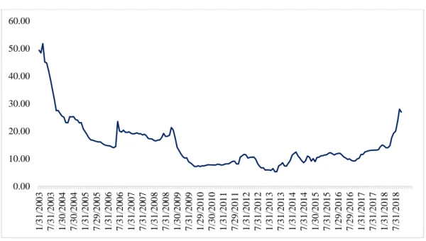
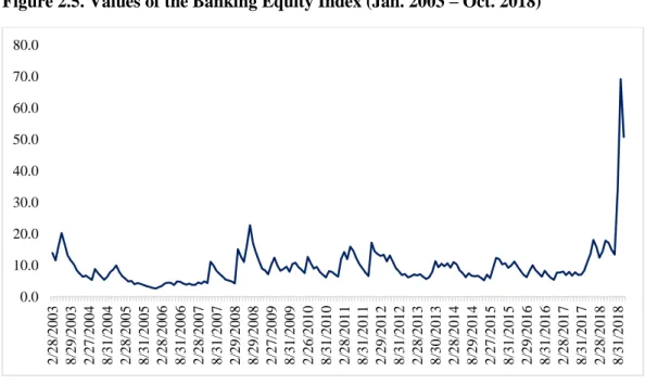
Figure 2.5. Values of the Banking Equity Index (Jan. 2003 – Oct. 2018) ... 24
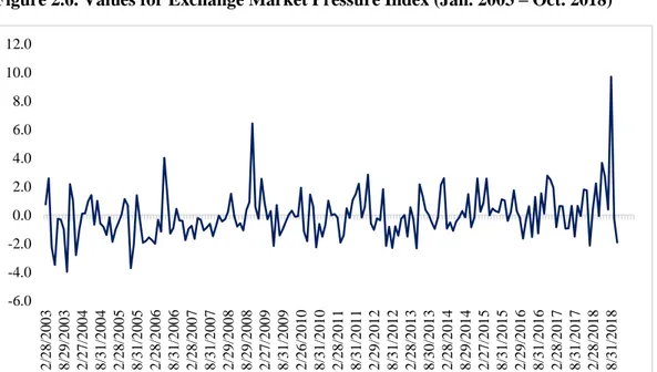
Figure 2.6. Values for Exchange Market Pressure Index (Jan. 2003 – Oct. 2018) 25 Figure 2.7. Values for Returns of BIST100 Index (Jan. 2003 – Oct. 2018) ... 27
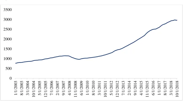
Figure 2.8. Values for Residential Sale Prices (Jan. 2003 – Oct. 2018) ... 28
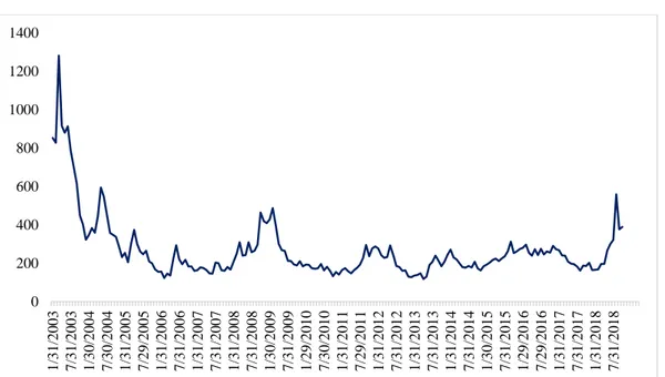
Figure 2.9. Values for 5-year CDS (Jan. 2003 – Oct. 2018) ... 29
Figure 2.10. Values for Government Bond Yield (Jan. 2003 – Oct. 2018) ... 30
Figure 3.1. Values for Standardized Variables (Jan. 2003- Oct. 2018) ... 33
Figure 3.2. Financial Stress Index for Turkey with Equal-Variance Weights Method ... 35
Figure 3.3. Financial Stress Index for Turkey with Principal Component Analysis ... 38
Figure 3.4. Financial Stress Index With Portfolio Theory ... 41
Figure 3.5. Comparison of the Financial Stress Indexes ... 42
Figure 4.1. Financial Stress Index for Turkey with Equal-Variance Weights Method with Residential Sale Prices ... 46
ix
Figure 4.2. Financial Stress Index for Turkey with Principal Component Analysis
with Residential Sale Prices ... 47
Figure 4.3. Financial Stress Index for Turkey with Portfolio Theory with Residential Sale Prices ... 48
Figure 4.4. Comparison of the Financial Stress Indexes with Residential Sale Prices ... 49
Figure A1. Principal Component Analysis EViews Output without Residential Sale Prices ... 55
Figure A2. Principal Component Analysis EViews Output with Residential Sale Prices ... 56
Figure A3. Volatility of BIST100 Index EViews Output ... 57
Figure A4. Volatility of Banking Sector Index EViews Output ... 58
Figure A5. Volatility of Currency Basket EViews Output ... 59
x
LIST OF TABLES
Table 2.1. The Model Selection Criteria Results for BIST100 Stock Market Returns ... 18
Table 2.2. The Model Selection Criteria Results for BIST100 Banking Sector Index ... 19
Table 2.3. The Model Selection Criteria Results for Currency Basket Indicator . 21
Table 2.4. Summary of The Variables ... 30
Table 2.5. Statistical Summary of Non-Standardized Variables (Jan. 2003 – Oct. 2018) ... 31
Table 3.1. Correlation Matrix for Variables in TFSI for the Period of January 2003 and October 2018 ... 36
Table 3.2. The Weights Extracted From the Principal Component Analysis ... 37
Table 3.3. The Results for Principal Component Analysis ... 37
Table 4.1. Correlation Matrix for Variables in TFSI for the Period of January 2003 and October 2018 with Residential Sale Prices ... 45
Table 4.2. The Weights Extracted From the Principal Component Analysis with Residential Sale Prices ... 46
Table 4.3. The Results for Principal Component Analysis with Residential Sale Prices ... 47
xi ABSTRACT
The aim of this study is to construct a financial stress index for Turkey by using different methods to evaluate whether the financial stress index that is constructed is successful in terms of predicting stressful time periods properly for the period between 2003-2018. In the literature, the measurement of the Financial Stress Index is commonly based on the banking sector, the foreign exchange market, the stock market, the bond market, and the public sector. Likewise, these indicators are used in this study, and also housing market indicator is added because deterioration in the housing market can have a systemic impact on the economy due to its relationship with the other markets. In this way, this study will contribute to the literature in terms of adding a relatively new variable in the measurement of financial stress. The 3-month TRLIBOR, foreign exchange market pressure index, the return of the Borsa Istanbul stock price index, 2-year government bond yields, Credit Default Swaps, and residential sales prices are the sub-components of the measurement of the financial stress in Turkey. The weighting scheme of those variables is based on three different methods. The equal-variance method is the most commonly used one which assumes every single market component has equal importance for all the financial system and also each component acts independently from each other. However, the principal component analysis takes into account the co-movement of the sub-market indicators in calculating financial stress. The standard portfolio theory considers the time-varying cross-correlations among the different stress indices. Furthermore, to measure volatilities for the banking sector equity index, currency, and the stock market, generalized autoregressive conditional heteroskedasticity models are used.
Keywords: Financial Stress, Equal-Variance Weight, Principal Component
iv ÖZET
Bu çalışmanın amacı farklı metodlar kullanarak Türkiye için bir finansal stres endeski oluşturmak ve 2003-2018 dönemi için oluşturulan bu stres endeksinin ilgili zaman aralığında stres dönemlerini doğru tahmin edip etmediğini araştırmaktır. Literatürde finansal stresin ölçümünde genel olarak bankacılık sektörü, döviz piyasası, hisse senedi piyasası, bono piyasası ve kamu sektörü kullanılmaktadır. Benzer şekilde bu çalışmada da bu piyasalar kullanılmış olup, ayrıca diğer piyasalarla etkileşimden dolayı sistemik etkiye sahip olduğu düşünülen konut fiyat endeksi çalışmaya dahil edilmiştir. Böylelikle finansal stresin ölçümünde görece yeni bir değişken eklenerek literature katkı sağlayacağı düşünülmüştür. 3-aylık TRLIBOR, döviz piyasası baskı endeksi, 2-yıllık devlet tahvili getirileri, Kredi Temerrüt Takası ve konut satış fiyatları Türkiye için finansal stresin ölçümünde kullanılan alt bileşenlerdir. Değişkenlerin ağırlıklandırılması üç farklı metoda dayanmaktadır. Her bir alt bileşenin birbirinden bağımsız hareket ettiğini ve eşit öneme sahip olduğunu varsayan eşit-varyans ağırlıklandırma metodu en yaygın kullanılandır. Bununla birlikte temel bileşenler analizi, alt piyasa göstergelerinin birlikte hareketini göz önünde bulundurur. Standard portföy teorisi ise farklı stres bileşenleri arasındaki zamana göre değişen çapraz korelasyonları dikkate alır. BIST bankacılık sektörü, hisse senedi endeksi, döviz piyasası ve BIS100 hisse senedi getirilerine ait volatilitelerin hesaplanmasında GARCH modelleri kullanılmıştır.
Anahtar Kelimeler: Finansal Stres, Eşit-Varyans Ağırlıklandırma, Temel
1
INTRODUCTION
Before the 1980s the studies about the financial sector focused mostly on only a single market rather than trying to draw a holistic picture of financial system. This situation has started to change after the late 1990s with the studies taking into consideration the interrelationship between different market segments. As a result, the financial stress indexes which include several variables from various sub-markets have been constructed (Ekinci, 2013).
There are several definitions of financial stress in the literature. It is defined as “the force that is exerted on economic agents by uncertainty, and changing expectations of loss in financial markets and institutions” by Illing and Liu (2003). Although Hakkio and Keeton (2009) mention the difficulty of defining financial stress specifically, they explain the common characteristics that different financial stress periods share. In those periods, there is an increase in the uncertainty with respect to the fundamental values of financial assets, which is a sign of an increase in the volatility of asset prices or the deterioration in the outlook of the economy as a whole. Uncertainty about the investor behavior also increases which again results in rising volatility in asset prices. Information asymmetry is another sign of financial stress. Furthermore, there is a transition from risky assets to safe assets. According to Hakkio and Keeton (2009), every period of financial stress comprises at least one of these features.
The global financial crisis has revealed the weaknesses in the financial system, and the importance of monitoring and supervising role of the regulatory authorities have increased. The ECB, FED, IMF, OECD, and BIS have developed the financial stress indexes for different countries to assess and monitor their current states of the
financial stability (Hakkio and Keeton, 2009; Cardarelli et al., 2011;Holló et al.,
2012). The studies which investigate the relationship between financial stress and economic activity have also become more important after the crises. Holló (2012), in his study of the Hungarian financial system, develops a financial stress index, a Composite Index of Systemic Stress (CISS), and shows that when the CISS exceeds
2
a certain threshold level, there is a decline in industrial production. Aboura and Van Roye (2013) in their study for France reach a similar conclusion that an increase in financial stress leads to lower economic activity. Same results can be found in Van Roye's (2013) study of the financial stress and economic activity in Germany. He argues that rise in financial stress is associated with a significant plunge in GDP growth. The studies searching the causes of financial stress do not treat the indicators of the stress independently, but create composite indexes reflecting the developments in many different market segments as a whole by considering the increased co-movements in those markets. In the literature, the measurement of the Financial Stress Index (FSI) is commonly based on five indicators; the banking sector, the foreign exchange market, the stock market, the bond market, and the public sector. Likewise, these indicators will be used in this study, and also another indicator - housing market which is an important component of the financial stress index will be added. In order to choose the appropriate variables to be the representatives of these six sectors, the study will refer to the related literature and will use the most commonly used variables. In that sense, firstly, in order to calculate the riskiness of the banking sector, interbank cost of borrowing which is represented by 3-month TRLIBOR will be used. The important thing in calculating the stress level in the banking sector is to consider the interbank liquidity constraints and the measurement of the default probability of the banking sector. Furthermore, some ratios such as non-performing loan ratio, loan-to-deposit ratio, etc. could be useful in evaluating the stress levels in different periods for this sector. Secondly, the volatility of the foreign exchange market will be calculated by considering the exchange rates and foreign reserves. For this, the foreign exchange market pressure index (EMPI) is commonly used. Stock market volatility which reflects the investor behavior will be measured by using the historical volatility of BIST100. For the representative of the stress in bond markets, two-year government bond yields are used. Another important component of the FSI is the public sector which is mostly measured by the Credit Default Swaps (CDS). This is an important indicator for investors to assess the economic conditions in the countries. The five-year CDS spreads can be used to measure the default risk of a sovereign. Furthermore,
3
sovereign bond spreads - the difference between Turkey’s 10-year government bond yield and 10-year US Treasury yield – can also be used. These are the main variables included in the measurement of FSI in Turkey. In addition to these variables, I will add the housing market because deterioration in the housing market can have a systemic impact on the economy due to its relationship with the other markets. After choosing the appropriate variables for Turkey, we need to decide which weighting scheme is better to explain the financial stress levels. The equal variance weight, the principal component analysis, and portfolio theory are the possible choices to be made. The equal-variance method is the most commonly used method which assumes every single market component has equal importance for the whole financial system. This method also assumes different sub-markets act independently from each other. However, the principal component analysis takes into account the co-movement of the sub-market indicators in calculating financial stress. However, the standard portfolio theory considers the time-varying cross-correlations among the different stress indices. I will calculate the FSI for these three different methods in order to see the differences in explaining power of the index. Apart from those, to measure volatilities generalized autoregressive conditional heteroskedasticity (GARCH (1,1)) models will be used.
In conclusion, the critical stress levels will be determined and it will be assessed whether the FSI that is calculated can be a good indicator for evaluating the economic conditions and estimating the stressful periods properly.
The remaining structure of the study is as follows. The first chapter includes the literature review. In the second chapter, the variables that are used in the measurement of the financial stress index for Turkey and the volatility measures are introduced. The construction and measurement of the financial stress index with three different approaches - equal-variance method, principal component analysis, and portfolio theory - is introduced in the following section. The fourth chapter includes the measurement of the financial stress index with the addition of the housing market indicator by using the same approaches in the third chapter. The conclusions and recommendations take place in the final part.
4 CHAPTER 1 LITERATURE REVIEW
As a representative of the financial stress, several indicators have been used since the 1980s. The slope of the yield curve, the credit risk, and the stock markets are some of them (Ekinci, 2013). However, the global financial crisis in the late 2000s in the US which spread over other countries has necessitated the detailed studies about the sources of financial stress. As a result, measuring financial stress can be seen as an attempt to elucidate the interrelations between the different market segments rather than focusing only on one indicator. However, there is no standard financial stress index which conforms to all countries or area that is investigated. Therefore, different indexes which reflect and consider the financial structure of the specific country examined have been developed. A financial stress index for developed countries is developed by Cardarelli et al. (2009). Balakrishnan et al. (2009), on the other hand, adapted it to the developing countries. Some of the indexes, in the literature, are country-specific (e.g., Illing and Liu, 2003; Holló, 2012; Aboura and Roye, 2013; Sun and Huang, 2016, Eraslan, 2017), some of them are constructed for several countries (e.g., Grimaldi, 2010; Roye, 2011; Paries et al., 2014; Vermeulen et al., 2014), and some of them investigate the relationship between the financial conditions and the economic activity (e.g., Hakkio and Keeton, 2009; Hatzius et al., 2010; Cardarelli et al., 2011). Financial stress indexes are also useful tools for policymakers for monitoring the financial stability, and make it possible to follow the sources of the stress, and provide alerts to risk managers to prevent or mitigate the effects of it (Oet et al., 2012).
Cardarelli et al. (2011) explored the effect of financial stress on the real economy. Their findings revealed that financial stress does not always result in an economic downturn, however, it often explains it properly. They constructed a financial stress index by using the variables from the banking, the securities, and the foreign exchange markets in 17 developed countries, but their particular attention was on the banking distress rather than the securities or the foreign exchange markets because of the longer recovery time requirement with related to the problems in the
5
banking sector. For them, more severe slowdowns in economic activities are associated with rapid credit expansion, rising housing prices, and increasing borrowing levels. They explain these downturns regarding the banking-dependent financial stress periods with the procyclicality of the leverage in the banking system in those countries.
A financial stress index for emerging economies (EM-FSI) is developed by Balakrishnan et al. (2009). They explicate the transition of financial stress from advanced to the emerging economies through trade and financial channels. According to them, profound changes in the asset prices, increases in uncertainty and risk, the liquidity constraints, and the stresses stemming from the banking sector are some of the main characteristics that the financial stress periods have in common. The index that they create includes the banking, the securities, and the exchange markets. Their contribution to the index that is developed by Cardarelli et al. (2009) is the inclusion of exchange market pressure index because it reflects the stress in emerging economies rather than the developed ones.
There are several studies which investigate the interaction between financial stress and economic activity. Hakkio and Keeton (2009) explain three possible ways that financial stress affects the real economy. When uncertainty about the financial asset prices rises, this would affect both households and the firm's decisions. In such a case, the household would prefer to delay their spending because of their future wealth concerns, businesses likewise would be more prudent about their investment and hiring decisions. Secondly, there may be an increase in financing cost through the rise in interest rates which in turn can lead both households and firms to decrease their spending, and the ultimate impact would be an additional deterioration in economic activity. Finally, financial stress may have an impact on diminishing economic activity through tightening credit standards of banks which means a further decline in spending. That is, during the times of financial crisis the willingness of banks to providing loan tendency will decline. The financial stress index – the Kansas City Financial Stress Index (KCFSI) – developed by Hakkio and Keeton explain the financial stress periods successfully and provides valuable
6
information about predicting changes in economic activity. Besides, it can also be a useful tool for policymakers in terms of making comparison possible with the current value of KCFSI and the known periods of financial stress in the previous periods. However, they do not provide an index which is capable of determining threshold levels of stress in the financial sector.
Elekdag and Kanlı (2010) analyze the relationship between financial stress and economic activity from the perspective of emerging markets. The impact of both external and internal financial stress shocks on Turkish economic activity is examined in a comparative way with the emerging economies. Their findings indicate that independent of being persistent or temporary, industrial production level is substantially affected by financial shocks which demonstrates the strong impact of financial stress on economic activity, is also proven with the latest global financial crisis. In their studies, they use a monthly composite index as an indicator of stress in the financial system. The comparative study of these authors reveals the sharper and faster contraction in the level of industrial production in Turkey after the global financial crisis. The sub-components of the index are foreign exchange market pressure index, comprising exchange rate and change in the level of central bank’s reserves, JPMorgan Emerging Market Bond Index Global (EMBIG), a benchmark index for the bond performance in emerging market countries, stock returns as a proxy for the stress in equity market and implied volatilities of stock returns as a benchmark for uncertainty perception relating to these stock returns in financial markets, and finally banking sector beta, an indicator of banking sector stress, which is based on Capital Asset Pricing Model (CAPM).
Kaya and Açdoyuran (2017), in their studies, fill a gap in the crises literature concentrating mostly on liquidity, banking, and debt crises but neglecting stock market. Since the volatility in oil prices not only affecting economic activity but also has a substantial impact on the financial sector, they incorporate that component to the financial stress index which they construct and examine the relationship between financial stress and oil prices with Autoregressive Distributed – Lagged (ARDL) Model. They follow Balakrishnan et al. (2009), Ekinci (2012),
7
Illing and Liu (2006), and Aklan et al. (2015) in deciding components of financial stress index. Accordingly, five-year credit default spread, stock returns, exchange market pressure index, and interbank cost of borrowing spread are used, and August 2002 – September 2015 period is examined with a monthly frequency. Their results indicate the usefulness of the index in predicting financial crises, and in providing beneficial information to policy makers in decision making.
Eraslan (2017) also analyzes the relationship between financial stress and economic activity. According to him, measuring financial stress is important for both determining economic policies and assessing the vulnerabilities in the financial system. To reflect the development in different market segments, he uses five different components to construct a financial stress index for Turkey for the period August 2002 – April 2016 with a daily frequency. These are the stock market, bond market, banking sector, foreign exchange market, and the public sector. As a proxy for the Turkish stock market, the return of Borsa Istanbul benchmark stock price index and the historical volatility of BIST100 are used. There are two variables, that Eraslan mentions in his study, to measure the stress in Turkish bond markets. One is the government bond spreads, which is the difference between Turkish two-year benchmark Treasury bond and US two-year Treasury bond, and another is Emerging Market Bond Index Plus (EMBI +), which represents total returns for traded external debt instruments, and is used as a benchmark for emerging market sovereign debt. 3-month LIBOR and idiosyncratic risk of the banking sector, measured by banking sector stock market volatilities, are the two instruments for evaluating the stress level in the banking sector. The volatility in the foreign exchange market is measured by the equally weighted average of USD and EUR. Finally, five-year USD denominated CDS spreads are used for the stress component of the public sector. Dynamic Principal Component Analysis is combined with Static Principal Component Analysis in this study to show the significance of using time-varying weights of financial market indicators, and the results indicate the capability of the financial stress index in identifying the financial stress episodes successfully, and can be a useful tool for early warning for risk in the Turkish economy.
8
Aklan, Çınar, and Akay (2015) also investigate the financial stress and economic activity relationship for Turkey. According to them, a system which enables the prediction of financial stress previously can reduce the possibility of financial crises
through the implementation of effective policy measures.The unfavorable impact
of potential stress sources can be eliminated owing to an early warning system. In this sense, a financial stress index, which comprises different market segments, i.e., stock markets, foreign exchange markets, banking sector, and public sector, is used in their study to measure and to monitor instabilities in Turkish financial system. The one-way causal relationship from financial stress to economic activity is found according to the Granger Causality Test, and the results indicate that for the period January 2002 – October 2014 economic activity contracts when there is an increase in financial stress in Turkey.
A similar study is conducted to reveal the relationship between financial stress and economic activity by Kaya and Kılınç (2017) for the period of August 2002 – September 2015 by using monthly frequency data. By following the literature (Illing and Liu, 2006; Balakrishnan et al., 2009; Ekinci, 2012; Aklan, 2015), they also constitute the financial stress index with the banking sector, foreign exchange market, security market, and public sector variables. Granger Causality Test and Vector Autoregressive (VAR) models are applied, and statistically significant relationship is found between financial stress and economic activity, which implies that financial stress index is successful in terms of reflecting crisis periods and directing economic activities.
Çamlıca (2016), on the other hand, constructs a composite index of systemic stress (CISS), combining the Central Bank of Turkey (CBRT)’s policy reaction function with a special financial stress index. He aims to measure the responsiveness of the CBRT’s monetary policy to financial stress during the period January 2005 and October 2015 by considering the cross-correlations between different market segments and by applying to CBRT’s policy interest rate. The variables of the index are money, credit, bond, equity, and forex markets. In estimating the CISS, the time-varying cross-correlations between different financial market segments are taken
9
into account. In this study, it is addressed that in the aftermath of the global financial crisis the importance of central banks’ roles in controlling financial risks in early stages is increased, and early warning mechanisms against financial instabilities have become important. That is, there is a change in the strategy of central banks after the global crisis from ‘clean after burst’, in which financial issues are mostly disregarded and price stability becomes the main concern, towards ‘lean against wind’, in which central banks have an effective role in intervening in financial crises and preventing financial risks. The empirical research is based on evaluating whether central bank’s responsiveness to financial stress has changed or not after heterodox tools that are used after mid-2010, and CBRT’s effort to achieve both financial and price stability at the same time during this period is an evidence that CBRT’s monetary policy is leaning more against financial stress compared to the previous period.
Çamlıca and Güneş (2016), in their studies, focus on methodological differences in measuring financial stress in Turkey. They apply the most widely used methods - equal variance weighting, principal component analysis, and portfolio theoretic weighting - in financial stress literature to compute the financial stress in Turkey for the period between 2002-2015. Their findings reveal the successful performance of these three different methods in explaining the financial stress terms during the period in question. To make a comprehensive study, they incorporate five sub-components to their index; the money market, the bond market, the banking sector, the security market, and the foreign exchange market. They also use daily frequency data to be able to reflect the real-time effects in financial markets. The comparison of the methods demonstrates the superiority of the portfolio theoretic weighting model among others in terms of taking time-varying correlations between sub-financial markets into consideration. Furthermore, this method considers the relations between financial stress and economic activity far more than other methods, and the recursive calculation provides a real-time index.
In this study, in addition to the main market segments that reflect the conditions of the financial system of Turkey, the residential sales prices are added to the financial
10
stress index. In the literature, there are some studies which incorporate that component to the index. Sun and Huang (2016) in their study constructed both financial stress index (CNFSI), which identifies the episodes of financial instability in China, and financial condition index (CNFCI), which provides information about the current financial state in China in order to measure the systemic risks. Their indices consist of four distinct markets which are banking, foreign exchange, stock, and debt markets. In order to find the contributing factors to the systemic financial stress, they suggest four leading indicators – credit, asset, monetary, and price – in addition to the main representors of China’s financial system. As a representative of those indicators growth rates of loans and deposits, house price index, growth rates of M2, and CPI inflation are used, and a combination of those indicators with CNFSI identifying the stress periods is an important step in terms of providing an early warning system for macroprudential regulations in China.
Kota and Saqe (2013), in their studies of the measurement of financial stress for Albania, also incorporate the variable of the housing market in addition to the banking sector, the money market, and the foreign exchange market since the problems in housing markets also have a tendency to lead to a systemic effect on the economy. Their study introduces the importance of taking into account using of an aggregated index which combines different market segments. Because by such an aggregated index the interaction between the markets can be followed, which makes it possible to follow systemic risk that is crucial for assessing the overall financial stability in a country. They define systemic risk as such that results in a financial system which is not well-functioning, and hindering economic growth and welfare by following Holló et al. (2011). According to them, increased uncertainty in financial markets which is reflected in terms of volatilities, liquidity constraints, the soundness of the banking sector, and the housing market trends are the common things that have to be considered when assessing the developments in financial markets. The effects of boom and bust in asset prices and credit growth on financial stability are analyzed in the literature in some studies. Borio and Lowe (2002), for example, discusses that in case of rapid credit growth, rapid increases in asset prices, and rapid increases in investment levels with simultaneous imbalances in
11
the other segments of financial markets stimulate the financial problems. The relation between asset prices, credit cycles, and developments in the real economy is revealed through their studies. Therefore, assessing the systemic impact of the deterioration in the housing market, that is the deviation of the housing price index from its trend, is an important tool for determining systemic stress, because, for Kota and Saqe (2013), it affects both financial systems via credit channel and real economy through the construction sector. That is, imbalances in the housing market would have a direct impact on other market segments.
Riiser (2005) in his study investigates some of the indicators that can be useful for forecasting banking crises in Norway. Correspondingly, he investigates the interrelation between asset prices and banking crises by applying to gap analysis, and the primary aim is to determine the indicators which have a predictive power of estimating banking-related crises. The argument is based on that during economic expansion, asset prices, and investment level increase, but that is not sustainable and at some point, the situation will reverse resulting in financial imbalances because of banks' ability to finance will be damaged. A similar study is conducted by Borio and Lowe (2002), and they evaluate the capability of the asset prices, credit to the private sector, and investment indicators in estimating banking crises at different time horizons. Their study reveals that credit gap alone is the best indicator in capturing stressful periods in the banking sector. On the other hand, a combination of these indicators improves the predictive ability and in that case credit gap together with real equity price give the best results. Riiser’s study is different in the sense that he also adds house prices to those indicators. His results show that before banking crises for the period that is analyzed there is mostly a visible increase in real house price gap - the percentage change of the deviation of HPI from its trend which is deflated by CPI - which implies that house price gap is successful in terms of capturing the crises periods in the banking sector.
The issue of predicting financial stress through observing the changes in credit and asset prices is also studied by Misina and Tkacz (2009). The aim is to provide leading indicators with regard to financial stress. Credit measures, asset prices,
12
macroeconomic variables, and foreign variables are the explanatory variables that they use. As credit measures, they use the growth rate of total household credit, total business credit, and total credit / GDP, and as asset prices, they use stock prices, commercial and residential real estate indices, the average price to personal disposable income ratio, and the Canadian dollar price of gold. The question of whether some combination of credit expansion and upward movement in asset prices can be used to forecast financial stress is investigated by them by applying to both linear and endogenous threshold models, and the result is affirmative depending on the model used and the forecast horizon. In particular, they found that the incorporation of business credit to the index causes some improvements in prediction performance of the financial stress in both linear and non-linear models at the one- and two- year horizons and their results suggest that the best predictor of the Canadian stress index is domestic credit growth at all horizons within a linear framework whereas asset prices are better predictors when it is allowed for nonlinearities. Their results show the difficulty of predicting financial stress. The relation between financial stress index (FSI) and financial crisis is studied by Vermeulen et al. (2014) for 28 OECD countries, and their results are different in the sense that they found a weak relationship between the start of a crisis and financial stress index. Their study, on the other hand, demonstrated the connection between FSI and the occurrence of a crisis. This relationship between financial stress and crises is also examined by Louzis and Vouldis (2013) in their study of developing a financial systemic stress index for Greece. They apply to the multivariate GARCH approach to capture the time-varying correlations between different markets. A survey is conducted for specifying the crises chronology for Greece among financial experts. According to the results, the index that they constructed is successful in identifying the crises periods and the stress levels in the Greek financial system.
There are several studies which investigate the negative relationship between financial stress and economic activity. Aboura and Van Roye (2013), in their study of the French economy, generated a financial stress index in order to evaluate the
13
real-time financial conditions with a dynamic approximate factor model. They mentioned three channels that financial stress has an impact on real economic activity; in stressful time periods banks’ willingness to lend decrease, firms postpone their investment decisions, and funding costs of the private sector increase. They analyzed this relationship by applying Markov – Switching Bayesian Vector Autoregressive Model (MS-BVAR) in order to identify the regime switching-between low-stress regime and high-stress regime. The financial stress index, industrial production growth, inflation rate, and the short-term interest rates are the variables that they use for identifying the regime switching. The FSI that they constructed captures the significant events in the French economy, and the results also indicate that if the economy is in a high-stress regime, the probability of financial stress to affect the economic activity increases, whereas in a low-stress regime economic activity is almost unaffected. Their ultimate results demonstrate the usefulness of the index as an early warning tool in the French financial system. In his study of Germany and the Euro area, Van Roye (2011), also used a dynamic factor model with regard to the construction of financial stress indicators. The impact of financial stress on business cycles is analyzed by applying to Bayesian VAR model (BVAR). According to the results, a significant decline in economic activity is associated with high financial stress.
The impact of financial stress on economic activity is also studied by Holló et al. (2011) by using econometric approaches – an autoregressive Markov-Switching model and a threshold bivariate VAR (TVAR) model, and their results also show that depending on the regime financial stress affects economic activity. That means in low-stress regime periods the effect of financial stress on economic activity is low whereas economic activity is highly affected when the economy is in a high-stress regime.
To evaluate the impact of financial stress shocks on real economic activity for Turkey, Güneş (2016), also applied a TVAR model by using the industrial production index as a representative of real economic activity. Since external shocks affect real economic activity more severely in high-stress regimes than the
14
low-stress regimes, the regime-dependent model was applied. In that sense, firstly TVAR model is estimated, then it is examined whether there is a threshold effect or not, and finally, impulse-response analysis is used to determine the asymmetric reactions caused by the financial stress shocks in both high- and low- stress regimes. The results revealed the negative effects of financial stress on economic activity. That is, industrial production is highly affected even in normal stress regimes. The impact, however, is more severe and prolonged in high-stress regimes.
None of the FSI studies on Turkey has used housing market as an indicator explaining the financial stress of the country. However, literature on various countries shows that house market index may be a significant variable in constructing FSI. Thus, the present study tries to fill this gap by using this additional variable in the construction of FSI for Turkey.
15 CHAPTER 2 METHODOLOGY
2.1. Construction of a Composite Index of Financial Stress
In the literature, different stress variableswhich reflect the characteristics of the
country investigated are used to construct the financial stress index. Following the previous literature in Turkey, this study also uses the banking sector, the foreign exchange market, the stock market, the public sector, and the bond market as the main sub-components to be in the construction of the index in Turkey. The variables are in monthly frequency and comprise the periods between January 2003 and
October 2018.The 3-month TRLIBOR, foreign exchange market pressure index,
the return of the Borsa Istanbul stock price index, 2-year government bond yields, 5-year Credit Default Swaps, and residential sales prices are the variables representing the relevant markets. Furthermore, to measure volatilities for the banking sector equity index, currency, and the stock market, generalized autoregressive conditional heteroskedasticity (GARCH) models are used.
2.1.1. Volatility Measures
The financial time series have three fundamental characteristics. These are heavy kurtosis, volatility clustering, and the leverage effect (Özden, 2008). It is assumed that if the financial time series have at least one of these properties, then the constant variance assumption is not valid. The traditional econometric models are based on the constant variance assumption. However, the homoskedasticity assumption is not sufficient to reflect the characteristics of financial time series. Therefore, ARCH-GARCH models are developed, considering changing variance in time. Engle (1982) developed the Autoregressive Conditional Heteroskedasticity (ARCH) model in order to reflect the dynamic characteristics of financial assets, and then Bollerslev (1986) developed the Generalized Autoregressive Conditional Heteroskedasticity Model, which is the extension of ARCH model. However,
16
positive and negative shocks have a different impact on volatility. The GARCH model does not take into account the asymmetric effects of positive and negative shocks. The effects of the shocks are determined independently of the sign of the shocks. Therefore, Nelson (1991) introduced the E-GARCH model. The GJR-GARCH model is an alternative model which also takes into account asymmetric effects, introduced by Glosten, Jagannathan, and Runkle (1993).
In this study, in measuring volatility, nonlinear conditional variance models, GARCH (1, 1), E-GARCH (1, 1), and GJR-GARCH (1, 1), are used. The reason for using these models is to see the effects of fluctuations in index that is investigated on variance, and then the appropriate model is chosen with certain criteria. The one with the highest R-squared value, or the one with the lowest Akaike Information Criterion or Schwarz Information Criterion value, or the one with the highest log-likelihood value will be chosen. For all volatility measures monthly logarithmic returns are used for the period 31.03.2003 and 31.10.2018. The stationarity tests are conducted with the Augmented Dickey-Fuller Test (ADF). After it is decided that the stationarity condition is satisfied, the best conditional mean equation is determined for all of the indexes. Then, the conditional variance models are estimated with the three different models.
2.1.1.1. Generalized Autoregressive Conditional Heteroscedasticity Models 2.1.1.1.1. GARCH (1, 1) Model
The conditional variance equation for GARCH (1, 1) model is as follows:
𝜎𝑡2 = 𝛼
0 + 𝛼1 𝑢𝑡−12 + 𝛽1𝜎𝑡−12 (2.1)
where 𝛼1 parameter shows the effect of shocks on the volatility, 𝛽1 parameter shows
the effect of the previous term volatility on the current term volatility. This equation is more successful in terms of capturing the volatility in financial asset returns data
17
compared to the ARCH (1) model1 because there is an additional term in this model
which takes into account that if there is large volatility in the previous time period, then the next time volatility will be predicted higher. That means large changes in asset prices will be followed by large changes and small changes will be followed by small changes, which is called volatility clustering.
2.1.1.1.2. GJR – GARCH (1, 1) Model
In this model, the variance changes depend on the size and/or the sign of the shock. Therefore, this is an asymmetric GARCH model. The conditional variance equation for this model is as follows:
𝜎𝑡2 = 𝛼0 + 𝛼1 𝑢𝑡−12 + 𝛾 𝑢𝑡−12 𝐼𝑡−1 + β 𝜎𝑡−12 (2.2)
where 𝐼𝑡−1 = 1 if 𝑢𝑡−1 < 0 and 0 otherwise. The parameter γ can be negative or
positive. The positive and statistically significant values of γ is an indicator of a leverage effect. That is, a large decrease in the price of a financial asset will affect the volatility of the returns more than a large increase within the price of a financial asset with the same magnitude.
2.1.1.1.3. E - GARCH (1, 1) Model
This is another asymmetric GARCH model. Again, the shocks will affect variance differently depending on the size or the sign of the shock. The conditional variance equation for this model is as follows:
ln (𝜎𝑡2) = 𝛼0 + β ln (𝜎𝑡−12 ) + γ 𝑢𝑡−1 √𝜎𝑡−12 + 𝛼1 (|𝑢𝑡−1 | √𝜎𝑡−12 ) (2.3) 1 𝜎 𝑡2 = 𝛼0 + 𝛼1 𝑢𝑡−12
18
There is also a leverage effect which implies that if γ is negative and statistically significant, then a decrease in returns will cause greater volatility than an increase in returns with the same magnitude.
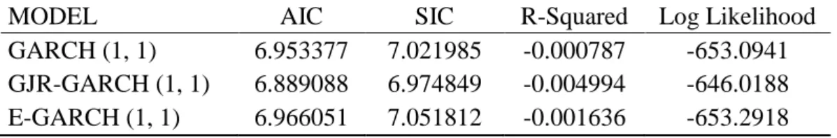
2.1.1.1.4. Volatility Measure for BIST100 Stock Market Returns
For monthly BIST100 Stock Market Returns, it is decided that GJR-GARCH (1, 1) is the most convenient model to apply. The results are as follows:
Table 2.1. The Model Selection Criteria Results for BIST100 Stock Market Returns
MODEL AIC SIC R-Squared Log Likelihood
GARCH (1, 1) 6.953377 7.021985 -0.000787 -653.0941
GJR-GARCH (1, 1) 6.889088 6.974849 -0.004994 -646.0188
E-GARCH (1, 1) 6.966051 7.051812 -0.001636 -653.2918
According to those results, GARCH parameter β (1.027655) is highly significant with p-values 0.0000, which indicates that the volatility in the previous time period will have an effect on the volatility in the next time period. The ARCH parameter
α1 (-0.074434) is significant at 1% level with p-values 0.0000, which indicates the
importance of the size of the shock on the volatility. The volatility of the BIST100 index has a positive contribution to the TFSI. The conditional variance equation for the BIST100 stock market returns are as follows:
𝜎𝑡 2 = 0.485220 – 0.074434 𝑢𝑡−12 + 1.027655 𝜎𝑡−12 + 0.058204 𝑢𝑡−12 𝐼𝑡−1 (2.4)2
19
Figure 2.1. The volatility of the BIST100 Index
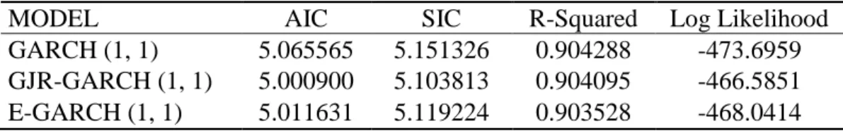
2.1.1.2. Volatility Measure for BIST100 Banking Sector Index
For monthly BIST100 Banking Sector Index, it is decided that GJR-GARCH (1, 1) is the most convenient method to apply. The results are as follows:
Table 2.2. The Model Selection Criteria Results for BIST100 Banking Sector Index
MODEL AIC SIC R-Squared Log Likelihood
GARCH (1, 1) 5.065565 5.151326 0.904288 -473.6959
GJR-GARCH (1, 1) 5.000900 5.103813 0.904095 -466.5851
E-GARCH (1, 1) 5.011631 5.119224 0.903528 -468.0414
According to those results, GARCH parameter β (0.873651) is highly significant with p-values 0.0000, which indicates that the volatility in the previous term has an impact on the volatility in the current term. In this way, if there is large volatility in the previous time period, then there will be a large amount of volatility in the next
time period. The ARCH parameter α1 (-0.031808), on the other hand, is not
significant at the 10% level with p-values 0.1752. The coefficient (γ) is positive with a value of 0.297232, which implies a leverage effect. It is also statistically
0.0 20.0 40.0 60.0 80.0 100.0 120.0 140.0 160.0 180.0 2 /2 8 /2 0 0 3 8 /2 9 /2 0 0 3 2 /2 7 /2 0 0 4 8 /3 1 /2 0 0 4 2 /2 8 /2 0 0 5 8 /3 1 /2 0 0 5 2 /2 8 /2 0 0 6 8 /3 1 /2 0 0 6 2 /2 8 /2 0 0 7 8 /3 1 /2 0 0 7 2 /2 9 /2 0 0 8 8 /2 9 /2 0 0 8 2 /2 7 /2 0 0 9 8 /3 1 /2 0 0 9 2 /2 6 /2 0 1 0 8 /3 1 /2 0 1 0 2 /2 8 /2 0 1 1 8 /3 1 /2 0 1 1 2 /2 9 /2 0 1 2 8 /3 1 /2 0 1 2 2 /2 8 /2 0 1 3 8 /3 0 /2 0 1 3 2 /2 8 /2 0 1 4 8 /2 9 /2 0 1 4 2 /2 7 /2 0 1 5 8 /3 1 /2 0 1 5 2 /2 9 /2 0 1 6 8 /3 1 /2 0 1 6 2 /2 8 /2 0 1 7 8 /3 1 /2 0 1 7 2 /2 8 /2 0 1 8 8 /3 1 /2 0 1 8
20
significant at 1% level with a p-value of 0.041. The existence of the leverage effect indicates that when there is a large decrease in the price of the financial asset, the return of the asset will be more volatile in the immediate future periods compared
to the large price increase with the same magnitude because of the parameter 𝐼𝑡−1.
In general, the volatility of the BIST100 index has a positive contribution to the TFSI. The conditional variance equation for the BIST100 banking sector index is as follows:
𝜎𝑡2 = 0.432919 – 0.031808 𝑢
𝑡−1
2 + 0.873651 𝜎
𝑡−12 + 0.297232 𝑢𝑡−12 𝐼𝑡−1 (2.5)3
Figure 2.2. Volatility of the Banking Sector Index
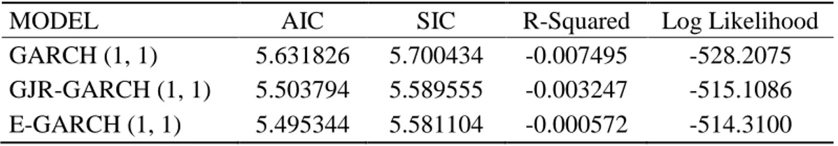
2.1.1.3. Volatility Measure For Currency Basket Indicator
For monthly Currency Basket Indicator (0.5 USD/TRY + 0.5 EUR/TRY), it is decided that E-GARCH (1, 1) is the most convenient method to apply due to the following results:
3 For details, see Figure A4.
0.0 10.0 20.0 30.0 40.0 50.0 60.0 70.0 80.0 90.0 100.0 2 /2 8 /2 0 0 3 8 /2 9 /2 0 0 3 2 /2 7 /2 0 0 4 8 /3 1 /2 0 0 4 2 /2 8 /2 0 0 5 8 /3 1 /2 0 0 5 2 /2 8 /2 0 0 6 8 /3 1 /2 0 0 6 2 /2 8 /2 0 0 7 8 /3 1 /2 0 0 7 2 /2 9 /2 0 0 8 8 /2 9 /2 0 0 8 2 /2 7 /2 0 0 9 8 /3 1 /2 0 0 9 2 /2 6 /2 0 1 0 8 /3 1 /2 0 1 0 2 /2 8 /2 0 1 1 8 /3 1 /2 0 1 1 2 /2 9 /2 0 1 2 8 /3 1 /2 0 1 2 2 /2 8 /2 0 1 3 8 /3 0 /2 0 1 3 2 /2 8 /2 0 1 4 8 /2 9 /2 0 1 4 2 /2 7 /2 0 1 5 8 /3 1 /2 0 1 5 2 /2 9 /2 0 1 6 8 /3 1 /2 0 1 6 2 /2 8 /2 0 1 7 8 /3 1 /2 0 1 7 2 /2 8 /2 0 1 8 8 /3 1 /2 0 1 8
21
Table 2.3. The Model Selection Criteria Results for Currency Basket Indicator
MODEL AIC SIC R-Squared Log Likelihood
GARCH (1, 1) 5.631826 5.700434 -0.007495 -528.2075
GJR-GARCH (1, 1) 5.503794 5.589555 -0.003247 -515.1086
E-GARCH (1, 1) 5.495344 5.581104 -0.000572 -514.3100
The statistically significant beta term at 1% level (0.0063) implies that past
volatility helps to predict future volatility. The ARCH term (α1), is also statistically
significant at 1% level, has a p-value of 0.0049, which implies that the size of the shock also has a significant impact on the volatility of the currency basket. The volatility of the currency basket has a positive contribution to the TFSI. The conditional variance equation for the currency basket is as follows:
ln (𝜎𝑡2) = 1.221541 + 0.337155 (|𝑢𝑡−1 | √𝜎𝑡−12 ) + 0.605133 𝑢𝑡−1 √𝜎𝑡−12 + 0.430395 ln (𝜎𝑡−1 2 ) (2.6)4
Figure 2.3. The volatility of the Currency Basket
4 For details, see Figure A5.
0.0 200.0 400.0 600.0 800.0 1000.0 1200.0 2 /2 8 /2 0 0 3 8 /2 9 /2 0 0 3 2 /2 7 /2 0 0 4 8 /3 1 /2 0 0 4 2 /2 8 /2 0 0 5 8 /3 1 /2 0 0 5 2 /2 8 /2 0 0 6 8 /3 1 /2 0 0 6 2 /2 8 /2 0 0 7 8 /3 1 /2 0 0 7 2 /2 9 /2 0 0 8 8 /2 9 /2 0 0 8 2 /2 7 /2 0 0 9 8 /3 1 /2 0 0 9 2 /2 6 /2 0 1 0 8 /3 1 /2 0 1 0 2 /2 8 /2 0 1 1 8 /3 1 /2 0 1 1 2 /2 9 /2 0 1 2 8 /3 1 /2 0 1 2 2 /2 8 /2 0 1 3 8 /3 0 /2 0 1 3 2 /2 8 /2 0 1 4 8 /2 9 /2 0 1 4 2 /2 7 /2 0 1 5 8 /3 1 /2 0 1 5 2 /2 9 /2 0 1 6 8 /3 1 /2 0 1 6 2 /2 8 /2 0 1 7 8 /3 1 /2 0 1 7 2 /2 8 /2 0 1 8 8 /3 1 /2 0 1 8
22 2.1.2. Variables
Choosing different market segments as the sub-components of financial stress, and incorporating the appropriate variables to the index requires considering certain criteria. Firstly, data must be available for a long period of time with a high frequency, and it has to encompass as much of the financial system volatility as possible. Namely, money markets, capital markets, banking sector, and foreign exchange markets (Holló et al., 2012) are good candidates in that sense. However, other market segments can also be included that is thought to be exploratory and to reflect the financial conditions of the specific country. Likewise, it is possible to extract unnecessary market segments that do not reflect country-specific characteristics. For example, Turkey is a country, which has experienced various
types of monetary policies since 2001.5 If we do not take into account the effects of
changing monetary policies on other financial indicators, in particular on exchange rates, we can get misleading results. That is, if exchange rates are not determined by the market, and exchange targeting regime is implemented, we cannot incorporate the foreign exchange market to the index (Ekinci, 2013). Therefore, it is important to choose a period when a certain policy is implemented consistently. Turkey has experienced many different monetary policies since 2000s. For the period between January 2000 and February 2001, exchange rate-based stability program is implemented. However, this system is terminated with the 2001 Crisis, which has resulted in some crucial structural changes in the monetary policy of Turkey. It is replaced with the floating exchange rate regime. Then, inflation targeting became the main objective of the CBRT and the implicit inflation targeting regime executed for the period between 2002-2005. After 2006 the CBRT adopted the explicit inflation targeting regime. In that sense, the variables that are
5 "Exchange rate peg between January 2000 and February 2001, the transition period between
February 2001 and December 2001, and dual targeting including monetary targeting and implicit inflation targeting between 2002 and 2005, and explicit inflation targeting between 2006 and today" (Ekinci, 2013).
23
chosen in this study cover the periods in which the consistent monetary policy is implemented, which is the inflation targeting after 2002.
2.1.2.1. Banking Sector
Incorporating the banking sector to the index is important because of its close relationship with the real economy. Under financial stress, banks cannot carry out their role of intermediation, and of providing credit and liquidity to the financial
systemproperly. In order to assess the soundness of the banking sector interbank
cost of borrowing, and the volatility of the banking sector will be used. As a proxy for the interbank cost of borrowing, three-month TRLIBOR is used by following Eraslan (2017).
Interbank cost of borrowingt = three-month TRLIBORt (2.7)
Figure 2.4. Values for 3-month TRLIBOR (Jan. 2003 – Oct. 2018)
To determine the bank-specific risk, that is the idiosyncratic risk of the banking sector, the volatility of the banking sector equity index is used. In determining the
0.00 10.00 20.00 30.00 40.00 50.00 60.00 1 /3 1 /2 0 0 3 7 /3 1 /2 0 0 3 1 /3 0 /2 0 0 4 7 /3 0 /2 0 0 4 1 /3 1 /2 0 0 5 7 /2 9 /2 0 0 5 1 /3 1 /2 0 0 6 7 /3 1 /2 0 0 6 1 /3 1 /2 0 0 7 7 /3 1 /2 0 0 7 1 /3 1 /2 0 0 8 7 /3 1 /2 0 0 8 1 /3 0 /2 0 0 9 7 /3 1 /2 0 0 9 1 /2 9 /2 0 1 0 7 /3 0 /2 0 1 0 1 /3 1 /2 0 1 1 7 /2 9 /2 0 1 1 1 /3 1 /2 0 1 2 7 /3 1 /2 0 1 2 1 /3 1 /2 0 1 3 7 /3 1 /2 0 1 3 1 /3 1 /2 0 1 4 7 /3 1 /2 0 1 4 1 /3 0 /2 0 1 5 7 /3 1 /2 0 1 5 1 /2 9 /2 0 1 6 7 /2 9 /2 0 1 6 1 /3 1 /2 0 1 7 7 /3 1 /2 0 1 7 1 /3 1 /2 0 1 8 7 /3 1 /2 0 1 8
24
volatility in the banking sector, GJR-GARCH (1, 1) model is applied. The model is as follows:
𝑟𝑡𝑏𝑎𝑛𝑘𝑖𝑛𝑔= µ + 𝑟𝑡𝐵𝐼𝑆𝑇100 + 𝑢𝑡 (2.8)
𝜎𝑡2 = 𝛼0 + 𝛼1 𝑢𝑡−12 + β 𝜎𝑡−12 + 𝛾 𝑢𝑡−12 𝐼𝑡−1 (2.9)
In those equations, the return for banking sector index is represented by 𝑟𝑡𝑏𝑎𝑛𝑘𝑖𝑛𝑔,
BIST100 return by 𝑟𝑡𝐵𝐼𝑆𝑇100, residuals by 𝑢
𝑡, and conditional variance by 𝜎𝑡2. The
formula in 2.2 shows therelative volatility in returns on bank stocks as opposed to
the returns on the overall stock market.
Figure 2.5. Values of the Banking Equity Index (Jan. 2003 – Oct. 2018)
2.1.2.2. Foreign Exchange Market
Fluctuations in exchange rates affect countries, in particular, the countries having a large amount of current account deficits and external debt. The firms in the real sector have also affected the volatilities in the exchange rates in case they use foreign-currency loans. Currency crises are associated with important devaluations
0.0 10.0 20.0 30.0 40.0 50.0 60.0 70.0 80.0 2 /2 8 /2 0 0 3 8 /2 9 /2 0 0 3 2 /2 7 /2 0 0 4 8 /3 1 /2 0 0 4 2 /2 8 /2 0 0 5 8 /3 1 /2 0 0 5 2 /2 8 /2 0 0 6 8 /3 1 /2 0 0 6 2 /2 8 /2 0 0 7 8 /3 1 /2 0 0 7 2 /2 9 /2 0 0 8 8 /2 9 /2 0 0 8 2 /2 7 /2 0 0 9 8 /3 1 /2 0 0 9 2 /2 6 /2 0 1 0 8 /3 1 /2 0 1 0 2 /2 8 /2 0 1 1 8 /3 1 /2 0 1 1 2 /2 9 /2 0 1 2 8 /3 1 /2 0 1 2 2 /2 8 /2 0 1 3 8 /3 0 /2 0 1 3 2 /2 8 /2 0 1 4 8 /2 9 /2 0 1 4 2 /2 7 /2 0 1 5 8 /3 1 /2 0 1 5 2 /2 9 /2 0 1 6 8 /3 1 /2 0 1 6 2 /2 8 /2 0 1 7 8 /3 1 /2 0 1 7 2 /2 8 /2 0 1 8 8 /3 1 /2 0 1 8
25
in the local currency, changes in reserve levels, and prominent changes in interest rates (Illing and Liu, 2003). Exchange market pressure index (EMPI) which includes both exchange rate depreciation and changes in international reserves will be used as a representative of the stress in the foreign exchange market (Balakrishnan et al., 2009). The formula for EMPI is as follows:
𝐸𝑀𝑃𝐼𝑡 = (𝛥𝑒𝑡−µ𝛥𝑒)
𝜎𝛥𝑒 –
(𝛥𝑅𝐸𝑆𝑡− µ𝛥𝑅𝐸𝑆)
𝜎𝛥𝑅𝐸𝑆 (2.10)
The changes in USD/TRY exchange rate is represented by 𝛥𝑒 and the changes in
international reserves for Turkey is represented by 𝛥𝑅𝐸𝑆. µ and σ denote the mean and standard deviation of the related variable, respectively. According to the formula 2.4, an increase in the real exchange rate and a decrease in reserves indicates that stress in the foreign exchange market escalates, and would have a negative impact on EMPI.
Figure 2.6. Values for Exchange Market Pressure Index (Jan. 2003 – Oct. 2018)
For capturing the stress in foreign exchange market, volatility of currency basket indicator, which comprises of equally weighted euro and dollar currencies (0.5 USD / TRY + 0.5 EUR / TRY), is also used. In measuring volatility of the currency
-6.0 -4.0 -2.0 0.0 2.0 4.0 6.0 8.0 10.0 12.0 2 /2 8 /2 0 0 3 8 /2 9 /2 0 0 3 2 /2 7 /2 0 0 4 8 /3 1 /2 0 0 4 2 /2 8 /2 0 0 5 8 /3 1 /2 0 0 5 2 /2 8 /2 0 0 6 8 /3 1 /2 0 0 6 2 /2 8 /2 0 0 7 8 /3 1 /2 0 0 7 2 /2 9 /2 0 0 8 8 /2 9 /2 0 0 8 2 /2 7 /2 0 0 9 8 /3 1 /2 0 0 9 2 /2 6 /2 0 1 0 8 /3 1 /2 0 1 0 2 /2 8 /2 0 1 1 8 /3 1 /2 0 1 1 2 /2 9 /2 0 1 2 8 /3 1 /2 0 1 2 2 /2 8 /2 0 1 3 8 /3 0 /2 0 1 3 2 /2 8 /2 0 1 4 8 /2 9 /2 0 1 4 2 /2 7 /2 0 1 5 8 /3 1 /2 0 1 5 2 /2 9 /2 0 1 6 8 /3 1 /2 0 1 6 2 /2 8 /2 0 1 7 8 /3 1 /2 0 1 7 2 /2 8 /2 0 1 8 8 /3 1 /2 0 1 8
26
basket, E-GARCH (1,1) model is applied according to the following formulas (Eraslan, 2017): 𝑟𝑡 = µ + 𝑢𝑡 (2.11) ln (𝜎𝑡2) = 𝛼0 + β ln (𝜎𝑡−12 ) + γ 𝑢𝑡−1 √𝜎𝑡−12 + 𝛼1 (|𝑢𝑡−1 | √𝜎𝑡−12 ) (2.12) 2.1.2.3. Stock Market
Equity crises are generally associated with steep declines in the overall market index in the literature. In such a case, the expected loss will rise, and there will be an increase in uncertainty regarding the returns of firms (Illing and Liu, 2003). There are several studies which incorporate stock market variables to the financial stress index (Illing and Liu, 2006; Balakrishnan et al., 2009; Cardarelli et al., 2009; Hakkio and Keeton, 2009; Ekinci, 2013; Vermeulen, 2014; Sun and Huang, 2016; Eraslan, 2017). Stress stemming from stock market-related events is seen as a crucial factor contributing to the financial crises. It is important to incorporate the variables in the index which take into account the time-varying characteristics of the asset price volatility. In that sense, in addition to Borsa Istanbul stock price index (BIST100), stock market return volatility is also used as a stress indicator in the equity market for Turkey.
27
Figure 2.7. Values for Returns of BIST100 Index (Jan. 2003 – Oct. 2018)
Forecasting volatility is crucial in order to counteract the risks in the financial markets. The volatility of BIST100 is measured by applying to the GJR-GARCH (1, 1) model.
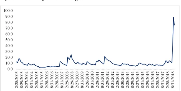
2.1.2.4. Housing Market
A steep increase in house prices can result in financial imbalances. Incorporating the housing market to the index can improve the predictive ability of crises. In that sense, following Kota and Saqe (2013) and Riiser (2005), the developments in the housing market is also monitored and the Residential Sale Prices are used as a proxy for this purpose. The beta of the housing sector is found with the following formula:
𝑟𝑡ℎ𝑜𝑢𝑠𝑖𝑛𝑔= µ + 𝑟𝑡𝐵𝐼𝑆𝑇100 + 𝑢𝑡 (2.13)
In this formula, the return for residential sale prices is represented by 𝑟𝑡ℎ𝑜𝑢𝑠𝑖𝑛𝑔,
BIST100 return by 𝑟𝑡𝐵𝐼𝑆𝑇100, and residuals by 𝑢𝑡. The formula in 2.13 shows the
-30.0 -20.0 -10.0 0.0 10.0 20.0 30.0 2 /2 8 /2 0 0 3 8 /2 9 /2 0 0 3 2 /2 7 /2 0 0 4 8 /3 1 /2 0 0 4 2 /2 8 /2 0 0 5 8 /3 1 /2 0 0 5 2 /2 8 /2 0 0 6 8 /3 1 /2 0 0 6 2 /2 8 /2 0 0 7 8 /3 1 /2 0 0 7 2 /2 9 /2 0 0 8 8 /2 9 /2 0 0 8 2 /2 7 /2 0 0 9 8 /3 1 /2 0 0 9 2 /2 6 /2 0 1 0 8 /3 1 /2 0 1 0 2 /2 8 /2 0 1 1 8 /3 1 /2 0 1 1 2 /2 9 /2 0 1 2 8 /3 1 /2 0 1 2 2 /2 8 /2 0 1 3 8 /3 0 /2 0 1 3 2 /2 8 /2 0 1 4 8 /2 9 /2 0 1 4 2 /2 7 /2 0 1 5 8 /3 1 /2 0 1 5 2 /2 9 /2 0 1 6 8 /3 1 /2 0 1 6 2 /2 8 /2 0 1 7 8 /3 1 /2 0 1 7 2 /2 8 /2 0 1 8 8 /3 1 /2 0 1 8
28
relative volatility in returns on housing as opposed to the returns on the overall stock market.
Figure 2.8. Values for Residential Sale Prices (Jan. 2003 – Oct. 2018)
2.1.2.5. Public Sector
As a representative of the public sector, Turkish five-year USD denominated credit default swaps (CDS), which shows the credit risk of the country, is used. The CDS is a protection against the borrower's default in return for a premium. That is, high levels of CDS premiums are associated with increased risk of default probability for sovereign debt. Increasing default probability leads to some problems on banks' balance sheet and the stress level in the financial system as a whole will be affected by that situation (Aboura and Roye, 2013). As a result, a high level of CDS contributes to TFSI positively.
0 500 1000 1500 2000 2500 3000 3500 1 /1 /2 0 0 3 8 /1 /2 0 0 3 3 /1 /2 0 0 4 1 0 /1 /2 0 0 4 5 /1 /2 0 0 5 1 2 /1 /2 0 0 5 7 /1 /2 0 0 6 2 /1 /2 0 0 7 9 /1 /2 0 0 7 4 /1 /2 0 0 8 1 1 /1 /2 0 0 8 6 /1 /2 0 0 9 1 /1 /2 0 1 0 8 /1 /2 0 1 0 3 /1 /2 0 1 1 1 0 /1 /2 0 1 1 5 /1 /2 0 1 2 1 2 /1 /2 0 1 2 7 /1 /2 0 1 3 2 /1 /2 0 1 4 9 /1 /2 0 1 4 4 /1 /2 0 1 5 1 1 /1 /2 0 1 5 6 /1 /2 0 1 6 1 /1 /2 0 1 7 8 /1 /2 0 1 7 3 /1 /2 0 1 8 1 0 /1 /2 0 1 8