IS S N 1 3 0 3 –5 9 9 1
A SIMULATION STUDY ON TESTS FOR ONE-WAY ANOVA UNDER THE UNEQUAL VARIANCE ASSUMPTION
ESRA YI ¼GIT AND FIKRI GÖKPINAR
Abstract. The classical F-test to compare several population means depends on the assumption of homogeneity of variance of the population and the nor-mality. When these assumptions especially the equality of variance is dropped, the classical F-test fails to reject the null hypothesis even if the data actu-ally provide strong evidence for it. This can be considered a serious problem in some applications, especially when the sample size is not large. To deal with this problem, a number of tests are available in the literature. In this study, the Brown-Forsythe, Weerahandi’s Generalized F, Parametric Boot-strap, Scott-Smith, One-Stage, One-Stage Range, Welch and Xu-Wang’s Gen-eralized F-tests are introduced and a simulation study is performed to compare these tests according to type-1 errors and powers in di¤erent combinations of parameters and various sample sizes.
1. INTRODUCTION
In applied statistics an experimenter wants to compare two or more populations measured using independent samples. The classical F- (CF) test is used under the assumption that the populations have normal distributions with the same variances. In this paper we consider the problem of comparing the means of k populations with the assumption of heteroscedastic variances.
The CF test fails to reject the null hypothesis even for large samples when the pop-ulation variances are unequal. This is a serious problem, especially for biomedical experiments in which one does not usually have large samples. In such applications each data point can be so vital and expensive. Alternative methods are developed due to this problem. Some of these test statistics’distribution is not known and the p-value can be found by simulation (Weerahandi, 1995; Weerahandi, 2004). There
Received by the editors June 25, 2010, Accepted: October. 26, 2010.
2000 Mathematics Subject Classi…cation. Primary 05C38, 15A15; Secondary 05A15, 15A18. Key words and phrases. Brown-Forsythe test, Generalized F-test, Parametric Bootstrap test, Scott- Smith test, One-Stage test, One-Stage Range Test, Classic F-test, Welch test, Xu-Wang test.
c 2 0 1 0 A n ka ra U n ive rsity
are a large number of approximate tests (Chen and Chen, 1998; Chen, 2001; Tsui and Weerahandi, 1989; Krishnamoorthy et al., 2006; Xu and Wang, 2007a, 2007b) and exact tests (Bishop and Dudewicz, 1981; Welch, 1951; Scott and Smith, 1971; Brown and Forsythe, 1974) in the literature. In practice, some exact procedures such as the CF, Welch (W), Scott-Smith (SS) and Brown-Forsythe (BF) tests are widely used. Alternative tests have been applied to solve a number of problems when conventional methods are di¢ cult to apply or fail to provide exact solutions. In this paper we carry out a simulation study to compare the size performance of the CF, W, SS, BF, Chen-Chen’s One Stage (OS), Chen-Chen’s One Stage Range (OSR), Weerahandi’s Generalized F (GF), Xu-Wang’s Generalized F (XW) and Parametric Bootstrap (PB) tests when population variances are unequal in one-way ANOVA problems. The type-I error rates and powers of the tests are compared us-ing Monte Carlo simulation usus-ing various sample sizes and under various parameter combinations.
2. TESTS FOR ONE-WAY ANOVA
Let Xi1; : : : ;Xinibe a random sample from N ( i; 2i) i=1,. . . ,k. The problem of
interest involves testing
H0: 1= 2= : : : = k H1: Not all is are equal i = 1; : : : ; k (2.1)
The standardized between-group sum of squares and the standardized error sum of
squares are given in (2.2) and (2.3) when 2
is are unequal. ~ Sb= ~Sb 21; : : : ; 2k = k X i=1 niXi2 2 i Pk i=1 niXi 2 i 2 Pk i=1 ni 2 i (2.2) ~ Se= k X i=1 niSi2 2 i (2.3) Most of the test statistics to test the equality of means under heteroscedasticity are based on the standardized between-group sum of squares and standardized error sum of squares. In the rest of this section test statistics are brie‡y introduced. In this section the W, SS and BF tests, whose distribution can be obtained theorically, are given. GF test and the XW test based on the generalized F-test, whose p-values are obtained by simulation, are given. The OS and OSR tests developed by Chen and Chen (1998, 2001) based on Bishop and Dudewicz’s (1981) two-stage procedure are investigated. Finally, the PB test developed by Krishnamoorthy et al. (2006) is discussed.
The Welch Test If wi=Sn2i
i, Welch (1951) gives the following test statistics.
W = ~ Sb S12; : : : ; Sk2 . (k 1) 1 + 2(k 2)k2 1 Pk i=1ni11 1 wi P wj 2 = Pk i=1wi h (Xi X)2 . (k 1)i 1+2 (kk2 12) Pk i=1ni 11 1 Pwiwj 2 (2.4)
If H0is true, then the distribution of W is Fk 1;f where
f = 1 3 k2 1 Pk i=1ni11 1 wi P wj 2
For a given level , and an observed value Wh of W, this test rejects the H0 in
(2.1) whenever the p-value is given as P (Fk 1;fi Wh) h .
The Scott-Smith Test
If S 2
i = nnii 13S
2
i, Scott and Smith (1971) give the following test statistics.
Fs= k X i=1 ni Xi X 2 S 2 i
If Hois true, then the distribution of Fsis 2k. For a given level , and an observed
value fs of Fs, this test rejects the H0 in (2.1) whenever the p-value is given as
P (Fsifs) h .
The Brown-Forsythe Test
Brown and Forsythe (1974) give the following test statistics.
B = k X i=1 ni Xi X 2 , k X i=1 1 ni n S 2 i
If H0is true, then the distribution of B is Fk 1;v; where
v = " k X i=1 1 ni n S 2 i #2, k X i=1 1 ni n 2 S4 i ni 1
For a given level , and an observed value Bhof B, this test rejects the H0in (2.1)
Weerahandi’s Generalized F-test
The sample variances (MLEs) of the k populations are denoted by Si2, where
Si2= 1 ni ni X i=1 Xij Xi 2 : De…ne Bj= Pj i=1 niSi2 2 i Pj+1 i=1 niS2i 2 i ; j = 1; : : : ; k 1
It follows from (2.3) that Bjis a beta random variable with parametersPji=1
(ni 1)
2 and
(nj+1 1)
2 and that ~Se, Bj are all independent random variables. Note also that the
random variables niSi2 2 i can be expressed as n1S12 2 1 = ~SeB1B2: : : Bk 1; niSi2 2 i = ~Se(1 Bi 1) Bi: : : Bk 1 for i = 2; : : : ; k 1 nkSk2 2 k = ~Se(1 Bk 1)
Therefore, the generalized p value can be expressed as
p = 1 E Hk 1;n k n k k 1~sb n1s21 B1B2: : : Bk 1 ; n2s 2 2 (1 B1)B2: : : Bk 1 ; : : : ; nks 2 k (1 Bk 1) (2.5)
where Hk 1;n kis the cumulative distribution function of the F -distribution with
k-1 and N-k degrees of freedom. This test rejects the H0 in (2.1) whenever ph
(Weerahandi, 1995a).
Xu-Wang’s Generalized F-test
For a bigger value of k the type-I error probability of the generalized F-test ex-ceeds the nominal level. Xu-Wang (2007a) developed some test statistics where its empirical type-I error probability does not exceed its nominal level.
Denote va= 1; 2; : : : ; k 1
0
and vb= 1k 1 k, where 1k 1 is the
(k 1) 1vector whose elements are all ones. Then null hypothesis in (2.1) is equal
to the null hypothesis as
The sample variances (MLEs) of the k populations are denoted by S2 i, where Si2= 1 ni ni X i=1 Xij Xi 2 . De…ne Ya = X1; : : : ; Xk 1 0 ; Yb= 1k 1Xk; Sa = diag S2 1 n1 1 ; : : : ; S 2 k 1 nk 1 1 Sb = 1 nk 1 Sk21k 11k0 1
Let ya, yb, sa and sb denote the observed values of Ya; Yb; Saand Sb respectively.
T is a generalized test variable as
T = Y0 (sa+ sb) 1=2 diag s2 1 U1 ; : : : ; s 2 k 1 Uk 1 + s 2 k Uk 1k 110k 1 (sa+ sb) 1=2 Y
and the observed value of T is given as
t = (ya yb)
0
(sa+ sb) 1(ya yb)
where Y N (0; Ik 1) ; Ui 2ni 1; i = 1; : : : ; k:
Under the null hypothesis in (2.1), the generalized p-value is given by
p = P (T t)
and H0 is rejected if p < .
The One-Stage Test
Chen and Chen (1998) developed the OS procedure since the number of samples that are required at the second stage of two-stage procedure of Bishop and Dudewicz (1981) can be large and impracticable.
For each population, the …rst (or any randomly chosen) n0(2 n0 ni) observation
is chosen to calculate the usual sample mean and variance as
Xi(n0) =Pnj=10 Xij n0 and S 2 i = Pn0 j=1 (Xij Xi(n0)) 2 (n0 1)
De…ne weights Ui and Vi for the observations in the i th sample as
Ui= n1i +n1i s ni n0 n0 S2 [k] S2 i 1 and Vi = 1 ni 1 ni s n0 ni n0 S2 [k] S2 i 1
Where S[k]2 is the maximum of (S12; : : : ; Sk2). Let the …nal weighted sample mean be
~ Xi= n X j=1 WijXij where Wij= Ui 1 j n0 Vi n0hj n
Chen and Chen (1998) give the following test statistics.
~ F1= k X i=1 ~ Xi X~ S[k] pn !2 Let ~X =Pki=1X~i k , = Pk i=1 ki and t = Pk i=1ti k = 1 k Pk i=1 ~ Xi i S[k]/pn = 1 S[k]/pn Pk i=1 ~ Xi i k = ~ X S[k]/pn Then we have ~ F1= k X i=1 ti t + i S[k] pn !2
Under the null hypothesis in (2.1), it follows that ~F1 is distributed as
Q = k X i=1
(ti t)2
which is a quadratic form in the independent student’s t variates each with n0-1
degrees of freedom (Chen and Chen, 1998). For a given level , and an observed
value ~Fh1of ~F1, this test rejects the H0 in (2.1) whenever the p-value is given as
P Qk;n0 > ~F
1
h < .
The One-Stage Range Test
In another procedure based on one stage, Chen (2001) gives the following test statistics. T1 = ~ Xmax X~min p z
where ~Xmax( ~Xmin) is the maximum (minumum) of ~X1; ; ~Xk and z* is the
max-imum of S12
n1; : : : ;
S2k
nk. Under the null hypothesis in (2.1), it follows that T1 is
R = max
1 i;j kj ti tjj
which is the range of k independent student’s t variates each with n0-1 degrees of
freedom. For a given level , and an observed value t1 of T1, this test rejects the
H0in (2.1) whenever the p-value is given as P (Rk;n0 1> t1) < .
A Parametric Bootstrap Approach
In the case of population variances 2
is are unknown; a test statistic can be obtained
by replacing 2 i in (2.2) by S2iand is given by ~ Sb S12; : : : ; Sk2 = k X i=1 niXi2 S2 i Pk i=1 niXi S2 i 2 Pk i=1 ni S2 i (2.6) As the test statistic in (2.6) is location invariant, without loss of generality, we can
take the common mean to be zero. Let XBi N 0;S
2 i
ni and S
2
Bi Si2 2ni 1 (ni 1).
Then the parametric boostrap pivot variable can be obtained by replacing X, S2
iin (2.6) by XBi, S2Biand is given by SbB= k X i=1 ni S2 Bi XBi2 " k X i=1 niXBi S2 Bi #2, k X i=1 ni S2 Bi (2.7)
XBi is distributed as Zi pSnii , where Zi is a standard normal random variable.
So the PB pivot variable in (2.7) is distributed as
~ SbB Zi; 2ni 1; S 2 i = k X i=1 Z2 i (ni 1) 2 ni 1 Pk i=1 pn iZi(ni 1) Si 2ni 1 2 Pk i=1 ni(ni 1) S2 i 2ni 1 H0is rejected if P n ~ SbB Zi; 2ni 1; s 2 i i ~sb o h (Krishnamoorthy, 2006). 3. SIMULATION STUDY
In this section we compare the CF, W, SS, BF, GF, XW, OS, OSR and PB tests according to type-1 errors and powers in di¤erent combinations of parameters and sample sizes.
3.1. Comparison between the type I error rates of the tests. In this section we consider the balanced and unbalanced cases from smaller to larger sample sizes where k =3 and k =5 for comparing the tests. The values for the variances vary over
a large range so that 2
1 < : : : < 2k and 21> : : : > 2k. For each combination of
ni and 2ithe rejection rate of each testing procedure is calculated and compared
with the nominal level 0.05 when the means are all equal. To estimate the type I error rates of the CF, W, SS, BF tests, we use simulation consisting of 5000 runs for each of the sample sizes and parameter con…gurations. CF, W, SS, BF test statistics are calculated from these generated data and type I errors are estimated by the proportion of test statistics that exceed the critical values calculated from the distributions. To estimate the type I error rates of the GF, PB, OS, OSR and XW tests, we use a two-step simulation. For estimating the type I error rates of
the GF test we generate 5000 observed vectors x1; :::; xk; s21; :::; s2k , and used 5000
runs for each observed vector to estimate the p value in (2.5). Finally the type I error rate of the GF test are estimated by the proportion of the 5000 p-values that
are less than the nominal level . The type I error rates of the PB, OS, OSR and
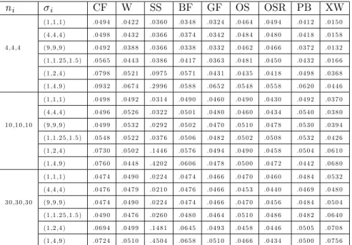
XW tests are similarly estimated. In both cases of equal and unequal variances for k=3 and k =5 simulated type I error probabilities are given in tables 1, 2, 3 and 4.
ni i CF W SS BF GF OS OSR PB XW (1 ,1 ,1 ) .0 4 9 4 .0 4 2 2 .0 3 6 0 .0 3 4 8 .0 3 2 4 .0 4 6 4 .0 4 9 4 .0 4 1 2 .0 1 5 0 (4 ,4 ,4 ) .0 4 9 8 .0 4 3 2 .0 3 6 6 .0 3 7 4 .0 3 4 2 .0 4 8 4 .0 4 8 0 .0 4 1 8 .0 1 5 8 4 ,4 ,4 (9 ,9 ,9 ) .0 4 9 2 .0 3 8 8 .0 3 6 6 .0 3 3 8 .0 3 3 2 .0 4 6 2 .0 4 6 6 .0 3 7 2 .0 1 3 2 (1 ,1 .2 5 ,1 .5 ) .0 5 6 5 .0 4 4 3 .0 3 8 6 .0 4 1 7 .0 3 6 3 .0 4 8 1 .0 4 5 0 .0 4 3 2 .0 1 6 6 (1 ,2 ,4 ) .0 7 9 8 .0 5 2 1 .0 9 7 5 .0 5 7 1 .0 4 3 1 .0 4 3 5 .0 4 1 8 .0 4 9 8 .0 3 6 8 (1 ,4 ,9 ) .0 9 3 2 .0 6 7 4 .2 9 9 6 .0 5 8 8 .0 6 5 2 .0 5 4 8 .0 5 5 8 .0 6 2 0 .0 4 4 6 (1 ,1 ,1 ) .0 4 9 8 .0 4 9 2 .0 3 1 4 .0 4 9 0 .0 4 6 0 .0 4 9 0 .0 4 3 0 .0 4 9 2 .0 3 7 0 (4 ,4 ,4 ) .0 4 9 6 .0 5 2 6 .0 3 2 2 .0 5 0 1 .0 4 8 0 .0 4 6 0 .0 4 3 4 .0 5 4 0 .0 3 8 0 1 0 ,1 0 ,1 0 (9 ,9 ,9 ) .0 4 9 9 .0 5 3 2 .0 2 9 2 .0 5 0 2 .0 4 7 0 .0 5 1 0 .0 4 7 8 .0 5 3 0 .0 3 9 4 (1 ,1 .2 5 ,1 .5 ) .0 5 4 8 .0 5 2 2 .0 3 7 6 .0 5 0 6 .0 4 8 2 .0 5 0 2 .0 5 0 8 .0 5 3 2 .0 4 2 6 (1 ,2 ,4 ) .0 7 3 0 .0 5 0 2 .1 4 4 6 .0 5 7 6 .0 4 9 4 .0 4 9 0 .0 4 5 8 .0 5 0 4 .0 6 1 0 (1 ,4 ,9 ) .0 7 6 0 .0 4 4 8 .4 2 0 2 .0 6 0 6 .0 4 7 8 .0 5 0 0 .0 4 7 2 .0 4 4 2 .0 6 8 0 (1 ,1 ,1 ) .0 4 7 4 .0 4 9 0 .0 2 2 4 .0 4 7 4 .0 4 6 6 .0 4 7 0 .0 4 6 0 .0 4 8 4 .0 5 3 2 (4 ,4 ,4 ) .0 4 7 6 .0 4 7 9 .0 2 1 0 .0 4 7 6 .0 4 6 6 .0 4 5 3 .0 4 4 0 .0 4 6 9 .0 4 8 0 3 0 ,3 0 ,3 0 (9 ,9 ,9 ) .0 4 7 4 .0 4 9 0 .0 2 2 4 .0 4 7 4 .0 4 6 6 .0 4 7 0 .0 4 5 6 .0 4 8 4 .0 5 0 4 (1 ,1 .2 5 ,1 .5 ) .0 4 9 0 .0 4 7 6 .0 2 6 0 .0 4 8 0 .0 4 6 4 .0 5 1 0 .0 4 8 6 .0 4 8 2 .0 6 4 0 (1 ,2 ,4 ) .0 6 9 4 .0 4 9 9 .1 4 8 1 .0 6 4 5 .0 4 9 3 .0 4 5 8 .0 4 4 6 .0 5 0 5 .0 7 0 8 (1 ,4 ,9 ) .0 7 2 4 .0 5 1 0 .4 5 0 4 .0 6 5 8 .0 5 1 0 .0 4 6 6 .0 4 3 4 .0 5 0 0 .0 7 5 6
Table 1.Simulated type I error rates when k=3 and sample sizes are equal under
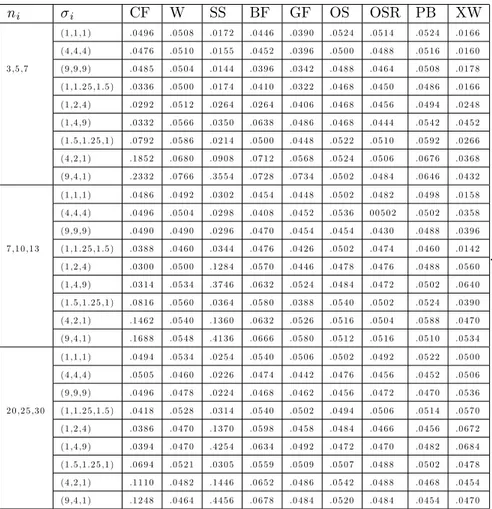
ni i CF W SS BF GF OS OSR PB XW (1 ,1 ,1 ) .0 4 9 6 .0 5 0 8 .0 1 7 2 .0 4 4 6 .0 3 9 0 .0 5 2 4 .0 5 1 4 .0 5 2 4 .0 1 6 6 (4 ,4 ,4 ) .0 4 7 6 .0 5 1 0 .0 1 5 5 .0 4 5 2 .0 3 9 6 .0 5 0 0 .0 4 8 8 .0 5 1 6 .0 1 6 0 3 ,5 ,7 (9 ,9 ,9 ) .0 4 8 5 .0 5 0 4 .0 1 4 4 .0 3 9 6 .0 3 4 2 .0 4 8 8 .0 4 6 4 .0 5 0 8 .0 1 7 8 (1 ,1 .2 5 ,1 .5 ) .0 3 3 6 .0 5 0 0 .0 1 7 4 .0 4 1 0 .0 3 2 2 .0 4 6 8 .0 4 5 0 .0 4 8 6 .0 1 6 6 (1 ,2 ,4 ) .0 2 9 2 .0 5 1 2 .0 2 6 4 .0 2 6 4 .0 4 0 6 .0 4 6 8 .0 4 5 6 .0 4 9 4 .0 2 4 8 (1 ,4 ,9 ) .0 3 3 2 .0 5 6 6 .0 3 5 0 .0 6 3 8 .0 4 8 6 .0 4 6 8 .0 4 4 4 .0 5 4 2 .0 4 5 2 (1 .5 ,1 .2 5 ,1 ) .0 7 9 2 .0 5 8 6 .0 2 1 4 .0 5 0 0 .0 4 4 8 .0 5 2 2 .0 5 1 0 .0 5 9 2 .0 2 6 6 (4 ,2 ,1 ) .1 8 5 2 .0 6 8 0 .0 9 0 8 .0 7 1 2 .0 5 6 8 .0 5 2 4 .0 5 0 6 .0 6 7 6 .0 3 6 8 (9 ,4 ,1 ) .2 3 3 2 .0 7 6 6 .3 5 5 4 .0 7 2 8 .0 7 3 4 .0 5 0 2 .0 4 8 4 .0 6 4 6 .0 4 3 2 (1 ,1 ,1 ) .0 4 8 6 .0 4 9 2 .0 3 0 2 .0 4 5 4 .0 4 4 8 .0 5 0 2 .0 4 8 2 .0 4 9 8 .0 1 5 8 (4 ,4 ,4 ) .0 4 9 6 .0 5 0 4 .0 2 9 8 .0 4 0 8 .0 4 5 2 .0 5 3 6 0 0 5 0 2 .0 5 0 2 .0 3 5 8 (9 ,9 ,9 ) .0 4 9 0 .0 4 9 0 .0 2 9 6 .0 4 7 0 .0 4 5 4 .0 4 5 4 .0 4 3 0 .0 4 8 8 .0 3 9 6 7 ,1 0 ,1 3 (1 ,1 .2 5 ,1 .5 ) .0 3 8 8 .0 4 6 0 .0 3 4 4 .0 4 7 6 .0 4 2 6 .0 5 0 2 .0 4 7 4 .0 4 6 0 .0 1 4 2 (1 ,2 ,4 ) .0 3 0 0 .0 5 0 0 .1 2 8 4 .0 5 7 0 .0 4 4 6 .0 4 7 8 .0 4 7 6 .0 4 8 8 .0 5 6 0 (1 ,4 ,9 ) .0 3 1 4 .0 5 3 4 .3 7 4 6 .0 6 3 2 .0 5 2 4 .0 4 8 4 .0 4 7 2 .0 5 0 2 .0 6 4 0 (1 .5 ,1 .2 5 ,1 ) .0 8 1 6 .0 5 6 0 .0 3 6 4 .0 5 8 0 .0 3 8 8 .0 5 4 0 .0 5 0 2 .0 5 2 4 .0 3 9 0 (4 ,2 ,1 ) .1 4 6 2 .0 5 4 0 .1 3 6 0 .0 6 3 2 .0 5 2 6 .0 5 1 6 .0 5 0 4 .0 5 8 8 .0 4 7 0 (9 ,4 ,1 ) .1 6 8 8 .0 5 4 8 .4 1 3 6 .0 6 6 6 .0 5 8 0 .0 5 1 2 .0 5 1 6 .0 5 1 0 .0 5 3 4 (1 ,1 ,1 ) .0 4 9 4 .0 5 3 4 .0 2 5 4 .0 5 4 0 .0 5 0 6 .0 5 0 2 .0 4 9 2 .0 5 2 2 .0 5 0 0 (4 ,4 ,4 ) .0 5 0 5 .0 4 6 0 .0 2 2 6 .0 4 7 4 .0 4 4 2 .0 4 7 6 .0 4 5 6 .0 4 5 2 .0 5 0 6 (9 ,9 ,9 ) .0 4 9 6 .0 4 7 8 .0 2 2 4 .0 4 6 8 .0 4 6 2 .0 4 5 6 .0 4 7 2 .0 4 7 0 .0 5 3 6 2 0 ,2 5 ,3 0 (1 ,1 .2 5 ,1 .5 ) .0 4 1 8 .0 5 2 8 .0 3 1 4 .0 5 4 0 .0 5 0 2 .0 4 9 4 .0 5 0 6 .0 5 1 4 .0 5 7 0 (1 ,2 ,4 ) .0 3 8 6 .0 4 7 0 .1 3 7 0 .0 5 9 8 .0 4 5 8 .0 4 8 4 .0 4 6 6 .0 4 5 6 .0 6 7 2 (1 ,4 ,9 ) .0 3 9 4 .0 4 7 0 .4 2 5 4 .0 6 3 4 .0 4 9 2 .0 4 7 2 .0 4 7 0 .0 4 8 2 .0 6 8 4 (1 .5 ,1 .2 5 ,1 ) .0 6 9 4 .0 5 2 1 .0 3 0 5 .0 5 5 9 .0 5 0 9 .0 5 0 7 .0 4 8 8 .0 5 0 2 .0 4 7 8 (4 ,2 ,1 ) .1 1 1 0 .0 4 8 2 .1 4 4 6 .0 6 5 2 .0 4 8 6 .0 5 4 2 .0 4 8 8 .0 4 6 8 .0 4 5 4 (9 ,4 ,1 ) .1 2 4 8 .0 4 6 4 .4 4 5 6 .0 6 7 8 .0 4 8 4 .0 5 2 0 .0 4 8 4 .0 4 5 4 .0 4 7 0 .
Table 2. Simulated type I error rates when k=3 and sample sizes are unequal
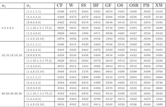
ni i CF W SS BF GF OS OSR PB XW (1 ,1 ,1 ,1 ,1 ) .0 4 8 6 .0 4 7 2 .0 4 9 4 .0 3 3 4 .0 6 1 8 .0 4 8 4 .0 4 8 0 .0 3 2 2 .0 1 6 2 (4 ,4 ,4 ,4 ,4 ) .0 4 8 0 .0 4 7 2 .0 4 7 2 .0 3 4 4 .0 5 6 8 .0 5 3 0 .0 5 3 8 .0 3 5 6 .0 1 2 0 (9 ,9 ,9 ,9 ,9 ) .0 4 6 2 .0 5 2 2 .0 5 1 0 .0 3 1 8 .0 6 4 0 .0 5 1 0 .0 5 1 6 .0 3 5 8 .0 1 0 8 4 ,4 ,4 ,4 ,4 (1 ,1 .2 5 ,1 .5 ,1 .7 5 ,2 ) .0 6 3 8 .0 6 3 4 .0 6 4 0 .0 4 4 2 .0 7 4 0 .0 4 9 4 .0 4 9 4 .0 4 7 0 .0 2 2 6 (1 ,2 ,4 ,6 ,8 ) .0 9 2 0 .0 8 0 4 .1 8 9 9 .0 5 7 1 .0 9 3 6 .0 4 6 5 .0 4 6 7 .0 5 2 8 .0 3 4 2 (1 ,4 ,9 ,1 3 ,1 8 ) .0 9 7 8 .0 8 5 6 .4 1 9 8 .0 5 5 6 .1 0 9 2 .0 5 3 8 .0 5 3 2 .0 5 8 0 .0 3 5 8 (1 ,1 ,1 ,1 ,1 ) .0 4 8 6 .0 5 1 8 .0 4 2 0 .0 4 6 8 .0 5 8 6 .0 5 1 6 .0 4 6 0 .0 4 9 6 .0 5 2 2 (4 ,4 ,4 ,4 ,4 ) .0 4 8 8 .0 5 2 0 .0 4 0 4 .0 4 7 0 .0 5 8 0 .0 4 9 2 .0 4 3 4 .0 4 9 4 .0 4 8 4 1 0 ,1 0 ,1 0 ,1 0 ,1 0 (9 ,9 ,9 ,9 ,9 ) .0 4 9 8 .0 5 4 8 .0 4 3 6 .0 4 8 8 .0 6 1 6 .0 4 9 8 .0 4 4 2 .0 5 0 6 .0 5 0 8 (1 ,1 .2 5 ,1 .5 ,1 .7 5 ,2 ) .0 6 2 6 .0 5 1 8 .0 4 9 4 .0 5 7 0 .0 6 1 0 .0 5 1 2 .0 5 1 8 .0 4 8 8 .0 5 8 6 (1 ,2 ,4 ,6 ,8 ) .0 8 5 2 .0 5 1 4 .1 8 4 4 .0 5 6 6 .0 6 4 4 .0 5 1 2 .0 5 1 8 .0 4 8 8 .0 7 6 0 (1 ,4 ,9 ,1 3 ,1 8 ) .0 8 8 0 .0 5 1 6 .5 4 7 6 .0 6 6 4 .0 6 8 4 .0 4 9 6 .0 4 9 0 .0 4 9 0 .0 7 6 8 (1 ,1 ,1 ,1 ,1 ) .0 4 9 4 .0 4 8 4 .0 3 0 0 .0 4 9 0 .0 5 1 0 .0 4 7 6 .0 5 0 4 .0 4 8 4 .0 6 6 6 (4 ,4 ,4 ,4 ,4 ) .0 4 9 4 .0 5 0 0 .0 3 1 0 .0 4 9 0 .0 5 3 8 .0 4 6 8 .0 4 7 2 .0 5 0 4 .0 7 3 6 (9 ,9 ,9 ,9 ,9 ) .0 5 0 4 .0 5 5 0 .0 3 1 8 .0 4 9 6 .0 5 7 0 .0 5 3 2 .0 5 2 8 .0 5 4 8 .0 6 8 8 3 0 ,3 0 ,3 0 ,3 0 ,3 0 (1 ,1 .2 5 ,1 .5 ,1 .7 5 ,2 ) .0 5 8 2 .0 4 8 4 .0 3 7 6 .0 5 6 2 .0 5 1 6 .0 4 9 0 .0 4 7 6 .0 4 8 8 .0 8 3 2 (1 ,2 ,4 ,6 ,8 ) .0 8 3 0 .0 4 9 4 .2 8 2 2 .0 7 9 0 .0 5 4 2 .0 4 7 4 .0 4 6 2 .0 4 7 0 .1 0 4 4 (1 ,4 ,9 ,1 3 ,1 8 ) .0 8 5 4 .0 5 0 2 .5 8 1 2 .0 8 1 4 .0 5 0 2 .0 5 3 8 .0 5 3 6 .0 4 8 6 .1 0 0 0 .
Table 3.Simulated type I error rates when k=5 and sample sizes are equal under
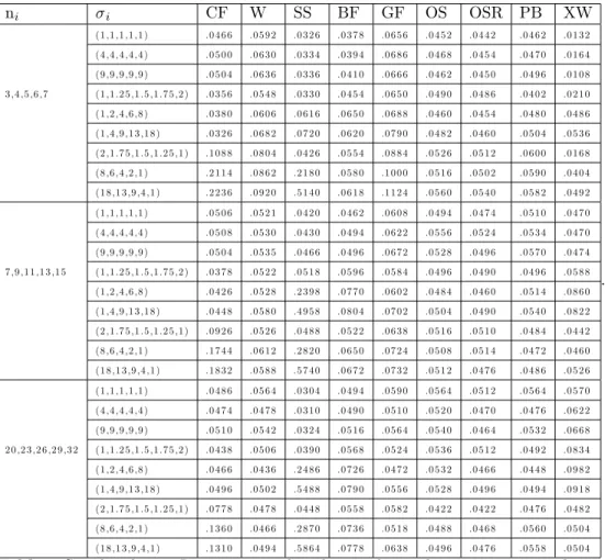
ni i CF W SS BF GF OS OSR PB XW (1 ,1 ,1 ,1 ,1 ) .0 4 6 6 .0 5 9 2 .0 3 2 6 .0 3 7 8 .0 6 5 6 .0 4 5 2 .0 4 4 2 .0 4 6 2 .0 1 3 2 (4 ,4 ,4 ,4 ,4 ) .0 5 0 0 .0 6 3 0 .0 3 3 4 .0 3 9 4 .0 6 8 6 .0 4 6 8 .0 4 5 4 .0 4 7 0 .0 1 6 4 (9 ,9 ,9 ,9 ,9 ) .0 5 0 4 .0 6 3 6 .0 3 3 6 .0 4 1 0 .0 6 6 6 .0 4 6 2 .0 4 5 0 .0 4 9 6 .0 1 0 8 3 ,4 ,5 ,6 ,7 (1 ,1 .2 5 ,1 .5 ,1 .7 5 ,2 ) .0 3 5 6 .0 5 4 8 .0 3 3 0 .0 4 5 4 .0 6 5 0 .0 4 9 0 .0 4 8 6 .0 4 0 2 .0 2 1 0 (1 ,2 ,4 ,6 ,8 ) .0 3 8 0 .0 6 0 6 .0 6 1 6 .0 6 5 0 .0 6 8 8 .0 4 6 0 .0 4 5 4 .0 4 8 0 .0 4 8 6 (1 ,4 ,9 ,1 3 ,1 8 ) .0 3 2 6 .0 6 8 2 .0 7 2 0 .0 6 2 0 .0 7 9 0 .0 4 8 2 .0 4 6 0 .0 5 0 4 .0 5 3 6 (2 ,1 .7 5 ,1 .5 ,1 .2 5 ,1 ) .1 0 8 8 .0 8 0 4 .0 4 2 6 .0 5 5 4 .0 8 8 4 .0 5 2 6 .0 5 1 2 .0 6 0 0 .0 1 6 8 (8 ,6 ,4 ,2 ,1 ) .2 1 1 4 .0 8 6 2 .2 1 8 0 .0 5 8 0 .1 0 0 0 .0 5 1 6 .0 5 0 2 .0 5 9 0 .0 4 0 4 (1 8 ,1 3 ,9 ,4 ,1 ) .2 2 3 6 .0 9 2 0 .5 1 4 0 .0 6 1 8 .1 1 2 4 .0 5 6 0 .0 5 4 0 .0 5 8 2 .0 4 9 2 (1 ,1 ,1 ,1 ,1 ) .0 5 0 6 .0 5 2 1 .0 4 2 0 .0 4 6 2 .0 6 0 8 .0 4 9 4 .0 4 7 4 .0 5 1 0 .0 4 7 0 (4 ,4 ,4 ,4 ,4 ) .0 5 0 8 .0 5 3 0 .0 4 3 0 .0 4 9 4 .0 6 2 2 .0 5 5 6 .0 5 2 4 .0 5 3 4 .0 4 7 0 (9 ,9 ,9 ,9 ,9 ) .0 5 0 4 .0 5 3 5 .0 4 6 6 .0 4 9 6 .0 6 7 2 .0 5 2 8 .0 4 9 6 .0 5 7 0 .0 4 7 4 7 ,9 ,1 1 ,1 3 ,1 5 (1 ,1 .2 5 ,1 .5 ,1 .7 5 ,2 ) .0 3 7 8 .0 5 2 2 .0 5 1 8 .0 5 9 6 .0 5 8 4 .0 4 9 6 .0 4 9 0 .0 4 9 6 .0 5 8 8 (1 ,2 ,4 ,6 ,8 ) .0 4 2 6 .0 5 2 8 .2 3 9 8 .0 7 7 0 .0 6 0 2 .0 4 8 4 .0 4 6 0 .0 5 1 4 .0 8 6 0 (1 ,4 ,9 ,1 3 ,1 8 ) .0 4 4 8 .0 5 8 0 .4 9 5 8 .0 8 0 4 .0 7 0 2 .0 5 0 4 .0 4 9 0 .0 5 4 0 .0 8 2 2 (2 ,1 .7 5 ,1 .5 ,1 .2 5 ,1 ) .0 9 2 6 .0 5 2 6 .0 4 8 8 .0 5 2 2 .0 6 3 8 .0 5 1 6 .0 5 1 0 .0 4 8 4 .0 4 4 2 (8 ,6 ,4 ,2 ,1 ) .1 7 4 4 .0 6 1 2 .2 8 2 0 .0 6 5 0 .0 7 2 4 .0 5 0 8 .0 5 1 4 .0 4 7 2 .0 4 6 0 (1 8 ,1 3 ,9 ,4 ,1 ) .1 8 3 2 .0 5 8 8 .5 7 4 0 .0 6 7 2 .0 7 3 2 .0 5 1 2 .0 4 7 6 .0 4 8 6 .0 5 2 6 (1 ,1 ,1 ,1 ,1 ) .0 4 8 6 .0 5 6 4 .0 3 0 4 .0 4 9 4 .0 5 9 0 .0 5 6 4 .0 5 1 2 .0 5 6 4 .0 5 7 0 (4 ,4 ,4 ,4 ,4 ) .0 4 7 4 .0 4 7 8 .0 3 1 0 .0 4 9 0 .0 5 1 0 .0 5 2 0 .0 4 7 0 .0 4 7 6 .0 6 2 2 (9 ,9 ,9 ,9 ,9 ) .0 5 1 0 .0 5 4 2 .0 3 2 4 .0 5 1 6 .0 5 6 4 .0 5 4 0 .0 4 6 4 .0 5 3 2 .0 6 6 8 2 0 ,2 3 ,2 6 ,2 9 ,3 2 (1 ,1 .2 5 ,1 .5 ,1 .7 5 ,2 ) .0 4 3 8 .0 5 0 6 .0 3 9 0 .0 5 6 8 .0 5 2 4 .0 5 3 6 .0 5 1 2 .0 4 9 2 .0 8 3 4 (1 ,2 ,4 ,6 ,8 ) .0 4 6 6 .0 4 3 6 .2 4 8 6 .0 7 2 6 .0 4 7 2 .0 5 3 2 .0 4 6 6 .0 4 4 8 .0 9 8 2 (1 ,4 ,9 ,1 3 ,1 8 ) .0 4 9 6 .0 5 0 2 .5 4 8 8 .0 7 9 0 .0 5 5 6 .0 5 2 8 .0 4 9 6 .0 4 9 4 .0 9 1 8 (2 ,1 .7 5 ,1 .5 ,1 .2 5 ,1 ) .0 7 7 8 .0 4 7 8 .0 4 4 8 .0 5 5 8 .0 5 8 2 .0 4 2 2 .0 4 2 2 .0 4 7 6 .0 4 8 2 (8 ,6 ,4 ,2 ,1 ) .1 3 6 0 .0 4 6 6 .2 8 7 0 .0 7 3 6 .0 5 1 8 .0 4 8 8 .0 4 6 8 .0 5 6 0 .0 5 0 4 (1 8 ,1 3 ,9 ,4 ,1 ) .1 3 1 0 .0 4 9 4 .5 8 6 4 .0 7 7 8 .0 6 3 8 .0 4 9 6 .0 4 7 6 .0 5 5 8 .0 5 0 4 .
Table 4.Simulated type I error rates when k=5 and sample sizes are unequal
under nominal =0.05
We observe the following from the numerical results in Tables 1, 2, 3 and 4. The CF and SS tests seem to have a type I error probability exceeding the nominal level for the balanced case and small sample sizes. In the case of extreme heteroscedasticity the W, BF, GF and PB tests exceed the nominal level. However, the OS, OSR and XW tests are superior to the other tests. The W, GF and PB tests also seem to be very conservative, when the sample sizes are large. The CF, SS and BF tests exceed the nominal level when the sample sizes are proportional to variances for small sample sizes. The W, GF, OS, OSR, PB tests seem to be very conservative not only for the small sample sizes but also for the large samples. However, the XW test exceeds the nominal level for the large sample sizes. The CF, W, BF, SS and GF tests exceed the nominal level when variances and sample sizes are inversly
proportional. However, the OS, OSR and XW tests seem to be very conservative. The W, GF and PB tests have similarly results when the sample sizes are large. For a bigger value of k the CF, W, SS, BF, GF tests exceed the nominal level when the sample sizes are small. The SS, BF and XW tests have similar results when the sample sizes are large. The OS, OSR and PB tests seem to be very conservative not only for the small sample sizes but also for the large sample sizes. For all cases similar results were found. It appears that the PB, OS and OSR tests are superior to the other tests.
3.2. Comparison Between The Powers Of The Tests. For each combination
of ni and 2ithe rejection rate of each testing procedure is calculated and compared
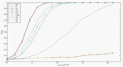
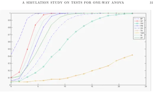
with the nominal level 0.05 when the means are not all equal. In this section we use 5000 runs for each of the sample sizes and parameter con…gurations to alculate the powers of the CF, W, SS, BF, OS, OSR, GF, PB, XW tests. For k=3 and k =5 we provide the powers of these tests.
Figure 1. Powers of the CF, W, SS, BF, OS, OSR, GF, PB, XW tests under
Figure 2. Powers of the CF, W, SS, BF, OS, OSR, GF, PB, XW tests under
nominal =0.05 for k =3, n=3, 5, 7 and 2
i=9, 4, 1
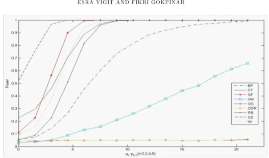
Figure 3. Powers of the CF, W, SS, BF, OS, OSR, GF, PB, XW tests under
Figure 4. Powers of the CF, W, SS, BF, OS, OSR, GF, PB, XW tests under
nominal =0.05 for k =5, n=3, 4, 5, 6, 7 and 2i=18, 13, 9, 4, 1
Figure 5. Powers of the CF, W, SS, BF, OS, OSR, GF, PB, XW tests for k =3,
n=20, 25, 30 and 2
Figure 6. Powers of the CF, W, SS, BF, OS, OSR, GF, PB, XW tests for k =3,
n=20, 25, 30 and 2
i=9, 4, 1
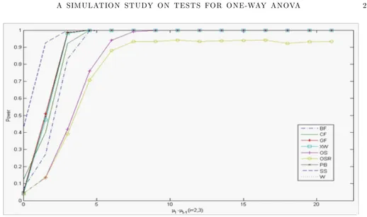
Figure 7. Powers of the CF, W, SS, BF, OS, OSR, GF, PB, XW tests for k =5,
n=20, 23, 26, 29,32 and 2
Figure 8. Powers of the CF, W, SS, BF, OS, OSR, GF, PB, XW tests for k =5,
n=20, 23, 26, 29,32 and 2
i=18, 13, 9, 4, 1
Figure 9. Powers of the CF, W, SS, BF, OS, OSR, GF, PB, XW tests under
Figure 10. Powers of the CF, W, SS, BF, OS, OSR, GF, PB, XW tests under
nominal =0.05 for k =3, n=30, 30, 30 and 2i=1, 4, 9
Figure 11. Powers of the CF, W, SS, BF, OS, OSR, GF, PB, XW tests under
nominal =0.05 for k =5, n=4, 4, 4, 4, 4 and 2
Figure 12. Powers of the CF, W, SS, BF, OS, OSR, GF, PB, XW tests under
nominal =0.05 for k =5, n=30, 30, 30, 30, 30 and 2
i=1, 4, 9, 13, 18
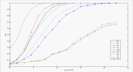
We once again observe from these …gures that the tests control the type I errors. The OS and OSR tests are badly a¤ected, especially with small and di¤erent sample sizes. These tests appear to be less powerful than the other tests although their type I error rates are close to the intended level 0.05. In most cases the SS test is disregarded because of its type I error rates exceeding the intended level 0.05. The other tests exhibit close power proporties provided the type I error rates are close to the intended level 0.05. Powers of tests become di¤erent from each other when the variances and sample sizes are inversely proportional for small sample sizes. These di¤erences increase, especially for bigger values of k. In most cases the GF, W and PB tests appear to be more powerful than the other tests. In particular, the GF test is superior to the other tests, except for small sample sizes and bigger values of k, because its type I error rates exceed the intended level 0.05. In this case the PB test is superior to the other tests.
4. CONCLUSION
In this simulation study for a range of choices of sample sizes and parameter con-…gurations we compared the performance of the above tests for testing the equality of means of one-way ANOVA models under heteroscedasticity. The CF test is not an appropriate test for heteroscedasticity because its type I error rates exceed the intended level 0.05. The same is true for the SS test. The OS and OSR tests appear to be less powerful than the other tests even though their type I error rates
are close to the intended level 0.05, regardless of the sample sizes, value of the error variances and the number of means being compared.
The W and PB and especially the GF tests appear to be more powerful than the
other tests when k =3 and the sample sizes are small (n1, n2, n3=3, 5, 7). The
W and PB tests are superior to the other tests when k =5 and the sample sizes
are small (n1, n2, n3=3, 5, 7). When the sample sizes are large the GF, W and
PB tests are more powerful than the other tests when both k =3 and k =5. In this case the XW test is also powerful when the variances and sample sizes are inversely proportional.
Although the empirical type I errors of the tests based on the OS procedure are close to their nominal level, the powers of these tests are not as high as those of the GF, W and PB tests. For this reason, the GF, W and PB tests can be used instead of tests based on the OS procedure.
ÖZET: ·Ikiden fazla y¬¼g¬n¬n ortalamalar¬n¬n e¸sitli¼gi hipotezinin
testi amac¬yla kullan¬lan klasik F testi, normallik ve y¬¼g¬n varyanslar¬n¬n
homojenlik varsay¬m¬na dayan¬r. Bu varsay¬mlar özellikle varyanslar¬n
homojenlik varsay¬m¬sa¼glanmad¬¼g¬nda klasik F testinin
kullan¬lma-s¬uygun olmamaktad¬r. Bu durum özellikle örneklem hacmi büyük
olmad¬¼g¬nda, önemli bir s¬k¬nt¬ do¼gurmaktad¬r. Literatürde bu
konuyla ilgili bir çok test istatisti¼gi geli¸stirilmi¸stir. Bu çal¬¸smada
Brown-Forsythe, Weerahandi’nin Genelle¸stirilmi¸s F, Parametrik
Bootstrap, Scott-Smith, One-Stage, One-Stage Range, Welch ve
Xu-Wang testleri tan¬t¬lm¬¸s ve testlerin farkl¬y¬¼g¬n
parametre-leri ve örnek hacimparametre-leri alt¬nda deneysel I.tip hata oran¬ ve testin
gücü bak¬m¬ndan kar¸s¬la¸st¬r¬lmas¬yap¬lm¬¸st¬r.
References
[1] Bishop, T.A. and Dudewicz, E.J. Heteroscedastic ANOVA, Sankhya 43B:40-57 (1981). [2] Brown, M.B., Forsythe, A.B. The small sample behavior of some statistics which test the
equality of several means, Technometrics 16: 129-132 (1974).
[3] Chen, S. and Chen, J.H. Single-Stage Analysis of Variance Under Heteroscedasticity, Com-munications in Statistics Simulations 27(??): 641-666 (1998).
[4] Chen, S. One stage and two stage statistical inference under heteroscedasticity, Communica-tions in Statistics SimulaCommunica-tions 30(??): 991-1009 (2001).
[5] Krishnamoorthy, K., Lu, F., Thomas, M. A parametric boostrap approach for ANOVA with unequal variances: …xed and random models, Computational Statistics and Data Analysis, 51:5731-5742 (2006).
[6] Weerahandi, S., ANOVA under unequal error variances, Biometrica, 38:330-336 (1995a). [7] Weerahandi, S., Exact statistical method for data analysis, Springer-Verlag, New York, 2-50
[8] Weerahandi, S., Generalized inference in repeated measures: Exact methods in MANOVA and mixed models, Wiley, New York, 1-60 (2004).
[9] Welch, B.L., The generalization of student’sproblem when several di¤erent population vari-ances are involved, Biometrika,3 4:28-35(1947).
[10] Welch, B.L., On the comparison of several mean values: An alternative approach, Biometrica, 38:330-336 (1951).
[11] Scott, A.J. ve Smith, T.M.F., Interval Estimates for Linear Combinations of Means, Applied Statistics, 20(??):276-285 (1971).
[12] Tsui, K. and Weerahandi, S., Generalized p-Values in Signi…cance Testing of Hypotheses in the Presence of Nuisance Parametres, Journal of the American Statistical Assocation, 84:602-607 (1989).
[13] Xu, L. and Wang, S. A new generalized p-value for ANOVA under heteroscedasticity, Statis-tics and Probability Letters, 78:963-969 (2007a).
[14] Xu, L. and Wang, S. A new generalized p-value and its upper bound for ANOVA under unequal erros variances, Communications in Statistics Theory and Methods, 37:1002-1010 (2007b).
Current address : Gazi University Faculty of Science and Art Depermant of Statistics Teknikokullar Ankara
E-mail address : [email protected]; [email protected] URL: http://communications.science.ankara.edu.tr