C om mun.Fac.Sci.U niv.A nk.Series A 1 Volum e 66, N umb er 2, Pages 243–252 (2017) D O I: 10.1501/C om mua1_ 0000000815 ISSN 1303–5991
http://com munications.science.ankara.edu.tr/index.php?series= A 1
A DISCRETE TIME MODEL FOR EPIDEMIC SPREAD: TRAVELING WAVES AND SPREADING SPEEDS
OZGUR AYDOGMUS
Abstract. In this paper, we aim to study spread of an epidemic in a spatially strati…ed population with non-overlapping generations. We consider mean …eld equation of an endemic chain-binomial process and allow individuals to dis-perse in the spatial habitat. To be able to model the spatial movement, we used an averaging kernel. The existence of traveling waves for traveling wave speeds greater than a certain minimum is proved. In addition, an explicit formula for the critical wave speed is given in terms of the moment generating function of the dispersal kernel and the basic reproductive ratio of the infectives.
1. Introduction
Mollison [14] modeled infectious disease spread by using a nonlocal contact model and this study triggered many other studies concerning the invasion of a new ter-ritory by intruder species. Mollison’s model does not allow individuals to disperse. Medlock and Kot [13] compared the nonlocal contact model and distributed infec-tives model. Both of these approaches assume that the dynamics of the populations under consideration are governed by continuous time processes.
On the other hand, discrete time models have also been used to model dynamics of epidemic processes [1, 2]. One of the most popular processes is the chain-binomial models(see for example [7, 11].) Chain binomial processes assume that the popu-lation has non-overlapping generations. Recently extinction time of a generalized endemic model with no immunity against the disease is studied using its mean …eld dynamics [5]. The mean …eld equation of the model, not surprisingly, is a di¤erence equation.
Ecological di¤erence equations with dispersal have been studied by Kot [9] in terms of traveling waves. Traveling waves in ecological processes are used to study invasion of a new habitat by an intruder species. Similarly in continuous time epi-demiological processes such solutions have been studied to determine the conditions
Received by the editors: October 12, 2016; Accepted: January 24, 2017.
2010 Mathematics Subject Classi…cation. Primary 05C38, 15A15; Secondary 05A15, 15A18. Key words and phrases. Epidemic, spread of infectives, asymptotic speed of propagation, trav-eling waves.
c 2 0 1 7 A n ka ra U n ive rsity C o m m u n ic a tio n s d e la Fa c u lté d e s S c ie n c e s d e l’U n ive rs ité d ’A n ka ra . S é rie s A 1 . M a th e m a t ic s a n d S t a tis tic s .
for invasion of a previously occupied habitat by infective individuals. For continu-ous time systems, the analysis of epidemic spread in terms of traveling waves and spreading speeds have been studied by many authors (see e.g. [17] and references therein.)
Here we consider the mean …eld equation of a generalized endemic chain-binomial process as given in [5] with spatial dispersal. This equation keep tracks of the frequency of infective individuals in discrete generations. We also allow individuals to disperse in the spatial habitat. The resulting equation is an integro-di¤erence equation describing an epidemic process with no immunity against the disease.
Given a spatially inhomogeneous epidemic model it is natural to look for traveling wave solutions. We show that there exists a critical traveling wave speed such that if the traveling wave speed exceeds this value there exists a solution connecting the disease free equilibrium and the endemic equilibrium. We also show that the model is linearly determinate, and thus we are able to give an explicit formula to calculate the critical wave speed in terms of the basic reproductive ratio of the model and the moment generating function of the dispersal kernel.
The paper is organized as follows: In section 2, we brie‡y introduce our model and some of its properties. In section 3, we give our main results concerning the invasion of the spatial habitat by infective individuals. In section 4, we provide simulation results concerning the model and verify that our theoretical …ndings are in accordance with the simulation results. In addition, the e¤ect of parameters, range of nonlocality and basic reproductive ratio, is investigated numerically. In section 5, we conclude our paper.
2. Model
Given a contact of a susceptible in period t; the probability that it is with an infective is {t= It=(N 1) where Itdenotes the number of infectives in a population
of size N: More generally, the probability that no e¤ective contact with susceptibles can be taken as a function of 1 {t: To de…ne the function we follow the method
suggested in [7] i.e. we assume that this function is a probability generating function of a discrete distribution and has the following form:
f (x) =
1
X
k=0
pkxk
where pk is the probability that a susceptible makes k contacts during a time
interval.
Assume that all infected individuals Itat time t will return to susceptible class
at time t + 1: In this case, there is no removed state so that St+ It= N for any
N 2 N where St is the number of susceptible individuals in the population. In
probability distribution: P r (It+1= xt+1jIt= xt) =
N xt
xt+1
(1 f (1 {t))xt+1(f (1 {t))N xt xt+1:
We consider the mean …eld equation of the above de…ned Markov process as following di¤erence equation:
it+1= (1 it)(1 f (1 it)) =: g(i): (2.1)
As an easy consequence of [5, Theorem 5], one can easily verify that for any " > 0 and T 2 N
lim
N!1P r( max1 n Tj{n inj > ") = 0
where {n= In=(N 1):
Hence, trajectories of the stochastic model and its mean …eld equation stay close to each other for any …nite time with probability 1. De…ne the basic reproductive number as follows:
= f0(1):
This value plays an important role in the dynamics of mean …eld equation (2.1). In [5], conditions for the existence and stability of an endemic equilibrium are given using the basic reproductive number as follows:
Theorem 1. [5] The following statements hold for any initial condition i02 (0; 1):
(i) If 1 then solutions to (2.1) approach the disease-free equilibrium i.e. limt!1it= 0:
(ii) If > 1 then solutions to (2.1) approach the unique endemic equilibrium ie2 (0;12) i.e. limt!1it= ie:
Equation (2.1) does not allow spatial movements of individuals. To be able to consider such movements, we denote the frequency of infective individuals at spatial location x and time t by it(x): Changes in these frequencies are modeled in two
alternating steps. In the …rst step it(x) is mapped into g(it(x)) The second stage
is spatial shu- ing. This stage is called dispersal stage and modeled by an integral operator. Hence the model is given as an integro-di¤erence equation of the form:
it+1(x) =
Z
k(x; y)g(it(y)) dy:
Here the kernel k(x; y) describes the dispersal of individuals from y: In particular, it is the probability that an infective individual in an interval of length dy about y disperses to an interval of the same length about x: Since k(x; y) is a probability kernel, it must be nonnegative. In a biological point of view, It is reasonable to assume that the dispersal weight depends on the relative distance i.e. k(x; y) = k(x y):
Here we assume also that the domain is in…nite and the redistribution or dispersal kernel has exponentially bounded tails. This is to say that the moment generating function of the probability kernel exists.
We state our standing assumptions on the probability generating function f and moment generating function of the dispersal kernel k as follows:
Assumption 1.
Random variables with probability generating function f and k have their …rst and second moments.
There exists a 0> 0 Z
R
e yk(y) dy < 1 for all j j 0:
Dispersal kernel k is piecewise continuous.
3. Traveling waves and spreading speeds Consider the following integro-di¤erence equation
it+1(x) = Q[it](x) :=
Z
R
k(x; y)g(it(y)) dy: (3.1)
Simple traveling waves are the solutions satisfying
it(x) = I(x ct) (3.2)
for some constant c: This constant is called traveling wave speed. In this setting, each iterate yields an extension of the solution with no change in the shape of it. Plugging the equation (3.2) in (3.1) one obtains
I(x c) = Z
R
k(x y)g(I(y)) dy: (3.3)
Here it is easy to see that the constant solutions to this equation are given by I = 0 and I = ie: Here we consider the traveling wave equation (3.3) with the following
boundary conditions:
I( 1) = ie and I(1) = 0: (3.4)
For the existence of such solutions see Appendix A. To be able to compute the critical wave speed explicitly we need to show the operator is linear determinate i.e.
g(i) i:
To be able to show this recall Bernoulli’s inequality:
for n 1: Using this, we have the following inequality: 1 f (1 i) 1 p0 1 X k=1 pk(1 ik) = i:
Thus we have g(i) i(1 i) < i for i 2 (0; 1):
Linear determinacy of this map implies that the critical wave speed can be characterized using the linearization of equation (3.1) near the equilibrium point 0 [19]. The critical wave speed c is the slowest value of the traveling wave speed c for which we can …nd a positive solution connecting two equilibria 0 and ie:
The linearization (or the Frechet derivative) of the of (3.1) near 0 is given by I(x c) = M[u](x) :=
Z
R
k(x y)I(y) dy: (3.5)
For a moving wave in negative direction, one can consider the following ansatz
I(x) = A exp( x) (3.6)
for positive. Plugging (3.6) in (3.5), one obtains the characteristic equation: exp( c) =
Z
R
k(s) exp( s) ds: (3.7)
Since we require that I(x) decussates the disease-free equilibrium 0; the appearance of such a solution coincides with the …rst appearance of a double root for (3.7). De…ne the following function
( ) = c log( ) log Z R k(s) exp( s) ds ! : (3.8)
First observe that 00(0) < 0 and hence we can conclude that 00( ) < 0 for all
j j 0 for some 0> 0: Thus the double root of this equation can be calculated
by taking = 0: Then, one can obtain a formula for the critical traveling wave speed which is given by
c = min >0 ( 1 log h Z R k(s) exp( s) ds i) (3.9) We have the following two results regarding the long time behavior of the model (3.3).
Theorem 2. If c c ; there exists solution of the equation (3.3) satisfying the boundary conditions (3.4).
The result follows from [19, Theorem 6.6] and hypotheses are veri…ed in Appendix A. This theorem implies that there exists a traveling wave solution connecting two equilibria 0 and ie: Biological interpretation of the result is that infectives in the
population cannot spread in the population if traveling wave speed is larger than the critical wave speed c :
To be able to get the whole picture we give the following result related to the operator (3.1) that informs us about both of the cases c < c and c > c :
Theorem 3. Suppose that the initial function 0 i0(x) 1 is zero for su¢ ciently
large x and i0(x) for some positive constant and all su¢ ciently negative x:
Then for any positive " the solution in(x) of the recursion (3.1) has the following
properties:
limn!1 supx n(c +")in(x) = 0;
limn!1 supx n(c ") ie in(x) = 0:
We used the theory developed in [10] to obtain above result and the conditions are veri…ed in Appendix A. The last limit tells us that infectives can spread at a speed no higher than the critical wave speed c :
4. Simulation studies
In this section, we turn to simulation studies on the e¤ects of model parameters on epidemic spread. We are interested in e¤ect of two parameters namely the basic reproductive number for the deterministic equation (2.1) and the range of nonlocality.
We concentrate on the normal distribution: k(x y) = p 1
2 2 exp
(x y)2
2 2 (4.1)
for simulation studies. This distribution is centered around zero and parameter characterizes the range of nonlocality. Here we also need to specify the discrete dis-tribution i.e. its mass function f: Here we use Poisson disdis-tribution for computation purposes. Hence we chose
f (x) = exp (1 x)
Thus our model without spatial dispersal can be read as
it+1= (1 it)(1 exp( it)): (4.2)
In our numerical simulations, we consider (3.3) corresponding to equation (4.2) with symmetric boundary conditions and use the discretization of the space variable 50 x 50 with a mesh interval of x = 0:01: The convolution terms is approximated by fast Fourier transform.
(a) (b)
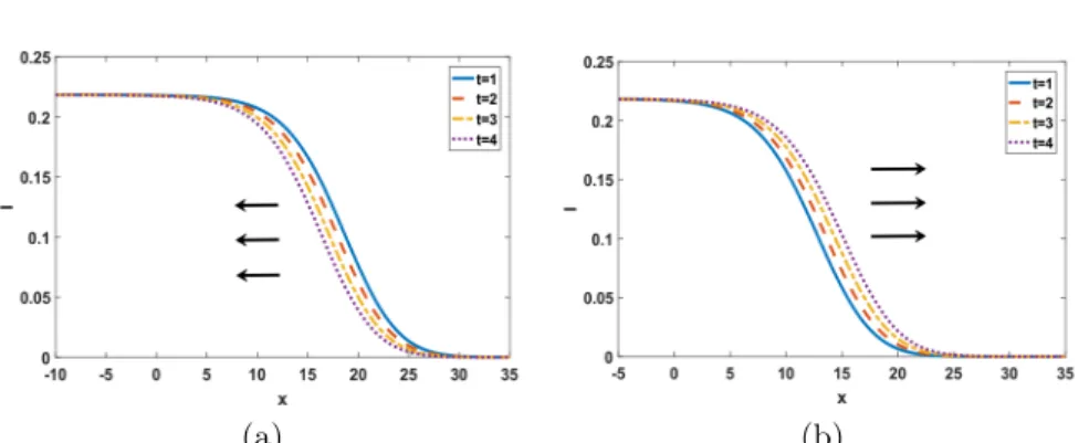
Figure 1. Panels (a) and (b) display the existence and non existence of traveling waves. The model parameters chosen here are = 1:5 and = 0:5: We set c = 2 for Panel (a) and c = 0:2 for panel (b).
For demonstration, we set = 1:5 and = 0:5: For these values, the critical wave speed can be calculated as c = 0:495 using the formula (3.9). Theorem 2 implies that traveling waves exist only for traveling wave speed c larger than this critical value. Panel (a) in Figure 1 shows the formation of a traveling wave whose front towards the negative direction as time evolves, and panel (b) suggests that no traveling waves along the negative direction are formed and the solution converges to constant ie on the domain. Hence, infective individuals spread in sustains in
panel (b) in Figure 1 and they diminish for large traveling wave speeds as shown in panel (a) of the same …gure.
Figure 2. E¤ect of the parameters and on the critical wave speed c . Here it is clear that the critical wave speed c measure the likelihood that infec-tives vanish in a population i.e. infection diminishes when the critical wave speed
is small. For our models (3.3) or (3.1), the critical speed is a function of two pa-rameters, namely the basic reproductive ratio and the range of nonlocality : To be able to further investigate and illustrate the e¤ect of these parameters we calculated the critical wave speed for a set of parameters. Here it is clear that the critical wave speed c measures the likelihood that infectives vanish in a popula-tion i.e. infecpopula-tion diminishes when the critical wave speed is small using the kernel function (4.1) with moment generating function exp( 2x2=2):
As seen in Figure 2, the critical waves speed increases with the parameters and : As expected, this implies that the higher rate of infection favors the spread of infectives. On the other hand, as the range of nonlocality gets larger, the spread of infectives is favored again.
5. Conclusion
In this paper, we considered spatial extension of an epidemic process derived as mean …eld equation of a stochastic process. The resulting equation is an integro-di¤erence equation modeling nonlocal dispersal of infective individuals.
We analyze the deterministic model on an unbounded region. We focus on studying traveling wave speed and/or the asymptotic speed of propagation. It has been shown that the model is linearly determinate which allows us to calculate the critical wave speed explicitly. Our main results can be summarized as follows:
(1) We investigate the critical traveling wave speed (or the spreading speed) as a function of extend of nonlocality of the dispersal kernel and the rate of infection. As a result, we found general conditions on the spread of infective individuals in terms of the critical traveling wave speed.
(2) We numerically studied the model and showed that the critical traveling wave speed increases as the range of nonlocality of the dispersal kernel and/or the rate of infection grows. Larger model parameters favors the spread of infectives.
One can extend these results to the multidimensional epidemic models using the theories developed in [10, 12]. These models include the multinomial AIDS models as presented in [18, pp. 89-92]. Another interesting question involves the study of asymptotic behavior of spatial generalization of SEIR type endemic processes with fractional time derivative [6, 15] .
Appendix A. Proof of Theorem 3
Here we sketch the proof of Theorem 3 by using the theory developed by Li et. all. [10] and Weinberger [19] Existence and uniqueness of solutions are clear. This also implies that map Q has semigroup property.
First of all note that for any constant ; Q[ ] = f ( ): In addition it is easy to show that f maps [0; 1] to itself. It was shown in [5, Theorem 1], f ( ) > for 2 (0; ie) and f ( ) < for 2 (ie; 1): Now we would like to note that the map Q
i. Suppose that u v ie a.e. for some u; v 2 B: Then we have
Q[u] Q[v] =
Z
R
k(x y) g u(y) g v(y) dy:
(A.1) Recall that the endemic equilibrium ies globally stable and hence the map
g is increasing for any function u ie: Then one can easily conclude that
g(u) g(v) 0 for any u v ie: Since the above given integrand is
non-positive, we have the order preserving property of the recursion as desired. ii. It is clear that for our model there are only two spatially homogeneous …xed points 0 and ie: It is easy to see that ie is an asymptotically stable …xed
point of Qtfor any constant initial condition by Theorem 1.
iii. If it(x) is a solution to equation (3.1) so does vt(x) = it(x y): Hence map
Q is translation invariant.
iv. Continuity can be obtained using [16, Theorem 5.3].
v. Existence of a subsequence vnk such that Q[vnk] converges uniformly on a
bounded set follows from Arzela-Ascoli theorem.
Consider the map Q and choose a continuous function with the following prop-erties:
(x) is non-increasing in x; (x) = 0 for all x 0;
0 ( 1) ie
To be able to de…ne the spreading speed, let a0(c; s) = (s) and de…ne the
sequence an(c; s) by the recursion;
an+1(c; s) = maxf (s); Q[an(c; s)](s + c)g: (A.2)
The above de…ned operator is also order preserving. By de…nition, it is easy to see that a1 a0= (s): It can be shown that an an+1 ieby induction. Moreover,
sequence an(c; s) is not increasing in c an s: Thus the sequence an converges to
a limit function a(c; s) non-increasing in c and s and bounded by ie: It follows
from Lui’s argument [12] that a(c; 1) are equilibrium of the map Q: In particular a(c; 1) = ie as noted in [10].
Now consider another initial condition ^ satisfying the above given properties. Hence there is another sequence ^an(c; s) whose limit function can be denoted by
^
a(c; 1): As discussed in [10], one can show that aN(c; x ) ^(x) for some
integer N and a translation : Hence, by comparison principle, it can be shown that ^a(c; 1) = a(c; 1): Hence we conclude that vector a(c; 1) is independent of the choice of the initial function : We then de…ne the slowest spreading speed by
Hence the result follows from [10, Theorem 2.2] for map Q: It is also possible to show that c+ is equal to critical traveling wave speed c given in (3.9) for the recursion (3.3) follows from [20, Theorem 3.4].
References
[1] Allen, L. J. S. Some discrete-time SI, SIR, and SIS epidemic models. Math. Biosci. (1994), 124(1), 83-105.
[2] Allen, L. J. S. ; Burgin, A.M. Comparison of deterministic and stochastic SIS and SIR models in discrete time. Math. Biosci. (2000), 163(1), 1-33.
[3] Aronson, D. G. The asymptotic speed of propagation of a simple epidemic. In Nonlinear Di¤ usion ; Fitzgibbon, W. E., Walker, H. F., Eds.; Pittman: London, UK, 1977; pp. 1-23. [4] Atkinson, C.; Reuter, G.E.H. Deterministic epidemic waves. Math. Proc. Camb. Philos. Soc.
(1976), 80(2), 315-330.
[5] Aydogmus, O. On extinction time of a generalized endemic chain-binomial model. Math. Biosci. (2016), 276, 38-42.
[6] Demirci, E.,Unal, A., Ozalp , N., A fractional order SEIR model with density dependent death rate, HJMS, (2011), 40, No. 2 287–295
[7] Jacquez, J. A. A note on chain-binomial models of epidemic spread: What is wrong with the Reed-Frost formulation?. Math. Biosci. (1987), 87(1), 73-82.
[8] Kendall D.G. Mathematical models for the spread of infection. In Mathematics and Computer Science in Biology and Medicine (1965) pp. 213-225.
[9] Kot, M. Discrete-time travelling waves: ecological examples. J. Math. Bio. (1992), 30.4, 413-436.
[10] Li, B.; Weinberger, H. F.; Lewis, M. A. Spreading speeds as slowest wave speeds for cooper-ative systems. Math. Biosci. (2005), 196.1 82-98.
[11] Longini, I. M. A chain binomial model of endemicity. Math. Biosci. (1980), 50.1, 85-93. [12] Lui, R. Biological growth and spread modeled by systems of recursions. I. Mathematical
theory. Math. Biosci. (1989), 93.2, 269-295.
[13] Medlock, J. and Kot, M., Spreading disease: integro-di¤erential equations old and new, Math. Biosci. (2003), 184.2, 201-222.
[14] Mollison, D. Spatial contact models for ecological and epidemic spread. J. Roy. Stat. Soc. B (1977), 283-326.
[15] Ozalp, N. and Demirci E., A fractional order SEIR model with vertical transmission, Math. and Comp. Mod. (2011), 54(1-2), 1-6.
[16] Precup, R., Methods in nonlinear integral equations, Springer Science & Business Media, 2013.
[17] Rass, L.; Radcli¤e, J., Spatial deterministic epidemics, American Mathematical Soc. Vol. 102., 2003.
[18] Tan W.Y., Stochastic models with applications to genetics, cancers, AIDS and other biomed-ical systems, World Scienti…c Vol. 4., 2002.
[19] Weinberger, H. F., Long-time behavior of a class of biological models. SIAM J. Math. Anal., 13.3, (1982), 353-396.
[20] Weinberger, H. F., Some deterministic models for the spread of genetic and other alterations. In Biological Growth and Spread, Springer, 1980; 320-349.
Current address : Ozgur Aydogmus: Department of Economics, Social Sciences University of Ankara.