PAIRS TRADING : BUILDING TRADING STRATEGIES
FOR ASSET PAIRS PRICE DYNAMICS
ÜMİT ÇETKİN
105625005
İSTANBUL BİLGİ UNIVERSITY
INSTITUTE OF SOCIAL SCIENCES
MASTER OF SCIENCE IN FINANCIAL ECONOMICS
UNDER SUPERVISION OF
PROF. DR. BURAK SALTOĞLU
Pairs Trading : Building Trading Strategies for Asset Pairs Price
Dynamics
Ümit ÇETKİN
105625005
Prof. Dr. Burak SALTOĞLU
:
Assoc. Prof. Dr. Ege YAZGAN
:
Dr.
Orhan
ERDEM
:
Approval
Date
: 07.08.2008
Number
of
Pages : 82
Keywords
Anahtar Kelimeler
1)
Pairs
Trading
1)
İkili Alım/Satım
2) Statistical Arbitrage
2) İstatistiksel Arbitraj
3) Market Neutral Strategy
3) Piyasa Nötr Strateji
4) Hedge Fund
4) Hedge Fon
ABSTRACT
In this thesis, we have studied Pairs Trading, which is a market neutral strategy built over the relative value of two similar assets. The strategy is implemented by identifying two assets whose prices tend to move together in long run and taking inverse positions in these two assets when there is a deviation from the long run relationship. In pairs trading, the trader does not make a bet on the direction of the stock prices, but invests in the condition of the asset prices relative to each other. In this study, we have analyzed the effects of pairs selection, threshold level selection and using bid/ask or low/high prices on the profitability of the strategy for Istanbul Stock Exchange stocks. The main implication of the study is that the portfolio formed with top 5 pairs with the lowest deviation between the normalized prices generates positive return most of the time and shows always the highest performance among the alternative portfolios. The only exception that the portfolio ends in loss is the liquidity crisis scenario where the model uses low/high prices for trade execution. However, the investor should bear in mind that there is no way to build totally risk neutral positions with Pairs Trading Strategy. There always remains the risk of break down of the relationship between the stocks and the liquidity risk that may be encountered in significant market downturns which is more important than the relationship between the stocks.
ÖZET
Bu tez çalışmasında, iki benzer kıymetin göreceli değerleri üzerine kurulmuş piyasa nötr bir strateji olan İkili Alım/Satım Stratejisi incelenmiştir. Strateji, fiyatları uzun dönemde birlikte hareket eden iki kıymetin tespit edilip uzun dönem ilişkisinden sapma olduğunda bu iki kıymette ters pozisyon alınması şeklinde uygulanır. İkili Alım/Satım’da yatırımcı hisse fiyatlarının yönüne değil, kıymet fiyatlarının birbirlerine göre olan konumlarına yatırım yapmaktadır. Bu çalışmada, İstanbul Menkul Kıymetler Borsası hisseleri için hisse seçimi, eşik değeri seçimi ve alış/satış veya en düşük/en yüksek fiyatların kullanımının strateji karlılığına etkileri incelenmiştir. Çalışmanın başlıca sonucu, normalize edilmiş fiyatlar arasında en düşük farka sahip en iyi 5 hisse ikilisi ile oluşturulan portföyün çoğunlukla pozitif getiri oluşturacağı ve alternatif portföyler arasında her zaman en iyi performansı göstereceği yönündedir. Porföyün zarar ile kapandığı tek istisna en düşük/en yüksek fiyatların işlem fiyatı olarak kullanıldığı likidite krizi senaryosudur. Ancak, yatırımcı İkili Alım/Satım Stratejisi ile, tam anlamıyla risk nötr pozisyon oluşturulması imkanının olmadığını göz önünde bulundurmalıdır. Hisseler arasındaki ilişkinin bozulması riski ve hisseler arasındaki ilişkiden daha önemli olan piyasanın ciddi çöküşlerinde yaşanacak likidite riski her durumda var olmaktadır.
ACKNOWLEDGEMENTS
I would like to express my gratitude to my supervisor Prof. Dr. Burak Saltoğlu, whose expertise and understanding added considerably to my study. I appreciate his knowledge, assistance and leading comments which helped me a lot in preparing my thesis. I would like to thank the other members of my thesis committee, Assoc. Prof. Dr. Ege Yazgan and Dr. Orhan Erdem for the assistance they provided.
I would like to thank to my mother, father and sister who have never stopped supporting. Their love and belief have been a great encouragement to me in every second of my life.
TABLE OF CONTENTS
1. INTRODUCTION ...1
1.1. Pairs Trading and Market Neutral Strategies...2
1.2. Emergence of Pairs Trading ...6
1.3. Role of Hedge Funds ...9
2. LITERATURE REVIEW ...15
3. METHODOLOGY ...23
3.1. Pairs Formation...24
3.2. Trading Period ...25
3.3. Return Calculation ...29
3.4. When does the Strategy Win or Fail? ...30
4. EMPIRICAL RESULTS...34
4.1. Strategy Performance...34
4.2. Trading Statistics ...41
4.3. Transaction Costs...45
4.4. Bid-Ask Spread...49
4.5. Liquidity Crisis Scenario ...54
5. RISKS WITH PAIRS TRADING STRATEGY ...58
6. SUMMARY ...64
7. CONCLUSION ...67
8. REFERENCES ...68
LIST OF TABLES
Table 1.1. Hedge Fund Investment Styles ...9
Table 1.2. List of Hedge Fund Losses with Market Neutral Strategies...12
Table 3.1. Summary of Trades for SKBNK-KRDMD Pair...31
Table 3.2. Summary of Trades for SKBNK-ARCLK Pair ...33
Table 4.1. Strategy Results with 2.0 Standard Deviation Threshold Level...35
Table 4.2. Strategy Results with 1.0 Standard Deviation Threshold Level...37
Table 4.3. Trading Statistics with Different Threshold Levels...41
Table 4.4. Strategy Results after 0.3% Transaction Cost with 2.0 Standard Deviations...45
Table 4.5. Strategy Results after 0.1% Transaction Cost with 2.0 Standard Deviations...46
Table 4.6. Decrease in Strategy Returns after Transaction Costs...49
Table 4.7. Strategy Results by using Bid/Ask Prices with 2.0 Standard Deviations...50
Table 4.8. Decrease in Strategy Returns by using Bid/Ask Prices ...53
Table 4.9. Strategy Results by using Low/High Prices with 2.0 Standard Deviations...55
LIST OF FIGURES
Figure 3.1. Sample Pairs Trading Strategy ...27
Figure 3.2. Sample Pairs Trading Strategy for SKBNK-KRDMD Pair ...30
Figure 3.3. Sample Pairs Trading Strategy for SKBNK-ARCLK Pair ...32
Figure 4.1. Average Returns of Pairs Trading Strategies ...38
Figure 4.2. Percentage of Pairs with Positive Return ...39
Figure 4.3. Average Number of Trades ...43
Figure 4.4. Average Number of Days in Position...44
Figure 4.5. Average Return for Top 5 Pairs after Transaction Costs ...47
Figure 4.6. Average Return for All Pairs after Transaction Costs...48
Figure 4.7. Average Return for Top 5 Pairs by using Bid/Ask Prices...51
Figure 4.8. Average Return for All Pairs by using Bid/Ask Prices ...52
Figure 4.9. Average Return for Top 5 Pairs by using Low/High Prices...56
Figure 4.10. Average Return for All Pairs by using Low/High Prices...56
APPENDICES
A.1. Table of Stocks ...74
A.2. Sample Trade Statistics...75
A.3. Performance of the Strategy...76
A.4. Average Return of Portfolios ...77
A.5. Percentage of Observations with Positive Return...77
A.6. Average Days in Position...78
A.7. Average Number of Trades...78
A.8. Average Return of Portfolios with 0.3% Transaction Cost ...79
A.9. Percentage of Observations with Positive Return with 0.3% Transaction Cost ...79
A.10. Average Return of Portfolios with 0.1% Transaction Cost ...80
A.11. Percentage of Observations with Positive Return with 0.1% Transaction Cost ...80
A.12. Average Return of Portfolios with Daily Bid/Ask Prices...81
A.13. Percentage of Observations with Positive Return with Daily Bid/Ask Prices...81
A.14. Average Return of Portfolios with Daily Low/High Prices...82
1. INTRODUCTION
In this thesis, we have tested the performance of Pairs Trading, a market-neutral trading strategy mainly implemented by hedge funds, on Istanbul Stock Exchange stocks. We have aimed to identify the effects of pairs selection, threshold level selection and using bid/ask or low/high prices on the profitability of the trading strategy.
In section 1, we have first described Pairs Trading Strategy and how the strategy emerged and became popular among the traders. Then, we have tried to understand the basics of market neutral strategies and arbitrage conditions. The main players of Pairs Trading Strategy, Hedge Funds, and the roles they have taken to increase the efficiency in financial markets have been mentioned. However, we have also summarized the biggest crashes of hedge funds in the history, such as LTCM case, which have to be taken into consideration and taken as lesson.
In section 2, we have reviewed the academic studies published about the market neutral strategies. There are many studies about different types of trading strategies those aim to build market neutral or risk-free profit opportunities. The studies cover mainly the stock markets and models are generally based on the price series of the stocks.
Section 3 covers the model we have built, which is mainly a partial replication of the strategy used in the study of Gatev et al. (2006). The model selects the portfolio of pairs according to the deviations between normalized price series of the stocks and opens inverse positions in two stocks when the deviation reaches the predetermined threshold level. In section 4, we have analyzed the empirical results of the trading strategy and compared the results in terms of portfolios and threshold levels. We have tested the robustness of the performance to transaction costs, which simulates a more realistic scenario. We also
replicated the model for different conditions such as using bid/ask prices or low/high prices in stead of daily close prices.
Although Pairs Trading Strategy is market neutral and expected to return profit with lower risk than traditional buy and hold strategies, there still remains the risk of losing money. The risks with Pairs Trading Strategy are covered in Section 5, which are due to the break down of the relationship between the stocks or market crash which results in the lack of liquidity.
1.1. Pairs Trading and Market Neutral Strategies
Pairs trading is a trading strategy that is built over the relative value of two assets, or a basket of assets, that allows traders profit from the anomalies between these assets’ prices. Although the strategy is generally formed to be market neutral by simultaneously buying and selling stocks from the same industry, market neutrality is not a necessity as long as the two stocks those invested have a strong relationship which may give the opportunity of exploiting any deviation from the long run relationship.
Pairs trading is implemented by identifying two assets whose prices tend to move together in long run and building trading strategy to gain profits while there exists a deviation in short run. In pairs trading, the trader does not make a bet on the direction of the stock prices, but exploits the probability of short run divergence.
The investor sells the stock that is thought to be overvalued and buys the other stock simultaneously, which is thought to be undervalued. As long as the strong relationship condition continues, one position should incur loss while the other position yields profit. However, if the relationship between these two stocks converges to equilibrium as expected, the net return of the position will be positive.
The benefit of pairs trading in this situation is that since the value of position in one stock is equal to the value of the position in the second stock, the strategy does not require any financing need, except the trading costs and short selling commissions for the margin account. Therefore, there exists an investment opportunity without any initial capital exposure. In addition, as the strategy is market neutral, the trader concentrates on the relationship between the two stocks instead of general market moves and performance of the strategy does not depend on the market direction.
Combined with fundamental analysis and improved computational and execution skills, pairs trading strategy is valuable for the investors who wants to earn more without betting in the market direction. Moreover, since the strategy can be implemented with a very low capital that will cover the margin maintenance and transaction costs, it is possible to use the advantages of leverage and gain significant profits. However, it is important to bear in mind that although the strategy is named as market neutral or an arbitrage strategy, there still remains the risk of firm specific events or market crashes which will make the investor lose more than a traditional buy and hold investment style. In addition, the relationship between the two assets may not be stable over time and the strategy investing in this relationship may unexpectedly fail.
Strategies like pairs trading are called “market neutral strategies” as these strategies do not bet on the direction of the market by buying or selling one asset and wait for the market to move in favor of the original position. The purpose of market neutral strategies is to find the portfolio of assets that will not be affected from the market movements and return excess profit with lower risk compared to the market.
Pairs trading is a simple form of market neutral strategies that is constructed by using just two securities, consisting of a long position in one security and a short position in another security, in a predetermined ratio. The portfolio is composed of securities having some kind of relationship that makes the securities move in a similar trend. The stocks with common
price dynamics decrease the riskiness of the portfolio return and make the whole investment market neutral.
There are two main types of pairs trading: Statistical Arbitrage Pairs Trading and Risk Arbitrage Pairs Trading.
Statistical Arbitrage Pairs Trading is based on the idea that assets with similar characteristics in terms of price dynamics must be priced similarly. Or, the assets having a relationship between each other that is stable in time should have similar market values. Any deviation from the long run relationship between the assets may be treated as mispricing between the two assets and it may be determined as an indicator to have a long position in the lower priced asset and a short position in the higher priced asset with the expectation of mispricing being eliminated when the relationship returns to its long run equilibrium.
Statistical arbitrage pairs trading can be implemented in different sectors and markets, or even with different assets. Since the strategy depends on the existence of long run relationship between the invested assets and the main determinant of this relationship is the comparison of historical price series of the assets, quantitative analysis of the asset price series is more important than the fundamental specifications of the assets. In addition, the market should allow short-selling and have enough liquidity as lack of these two conditions will make the implementation of statistical arbitrage pairs trading impossible.
Risk Arbitrage Pairs Trading, on the other hand, can be formed in case of a merger or acquisition between two companies. The terms of the merger agreement establish a parity relationship between the values of the two stocks of the two firms involved in the merger. The trade decision can be made for risk arbitrage when there is a significant deviation from the defined parity relationship. Investor analyzes the two securities involved in the merger, buys the lower priced security and sells the higher priced security. As a result, the portfolio
manager invests in the price parity and locks the price difference between the stocks before the merger is finalized.
Risk arbitrage pairs trading is possible when both securities in merger process are publicly traded in the open market while the merger is announced. Since risk arbitrage pairs trading requires understanding the merger process and details of the agreement, it is more than just analyzing the price movements of the stocks and requires additional evaluation skills. The investor should be well informed about fundamentals of the companies attending the merger process and be capable of pricing the whole trade with insights of corporate finance. The strategies which are searching for a riskless portfolio with positive return over market anomalies ended up in the introduction of the term “arbitrage”. There are some conditions to be satisfied to call a strategy as arbitrage. The transaction should have a positive probability of a positive payoff, a zero probability of a negative payoff, and the cost of the transaction should be zero, or at least there should be certain profit that will compensate the transaction costs. Statistical arbitrage pairs trading, on the other hand, is not riskless in general. However, there is positive expected payoff and zero probability of negative payoff only as time approaches infinity.
According to the definition introduced by Hogan et al. (2003), a self financing, zero-cost strategy that satisfies the following four conditions is called Statistical Arbitrage:
1. Discounted profit should be zero at t0,
2. The expected discounted profit should be positive, or at least be equal to risk-free rate, as time goes to infinity,
3. The probability of having negative expected discounted profit should be zero, as time goes to infinity,
4. A time averaged variance converges to zero when there is positive probability of a loss at every finite point in time, which could be achieved through portfolio rebalancing or
controlling the value of long and short positions to avoid excessive net exposure either long or short, as time goes to infinity.
Although the pairs trading strategy is a statistical arbitrage strategy and it has a positive expected profit as time goes to infinity, the strategy includes the low probability of a huge loss in case the relationship between the pair stocks crashes when the trader is holding a position. Therefore, Holton (2003) described strategies having high probability of making a little money and a low probability of losing a lot as “negatively skewed trading strategies”. The pairs trading strategy is described as market neutral and having a consistent profit performance. However, if the market dynamics change and the long run equilibrium relationship among the stocks disappears, the investment will result in a loss that can be much higher than it is imagined.
The reason for the market neutral strategies being popular among the quantitative traders is that returns of these strategies are independent and uncorrelated with the market regardless of the economic bubbles or downturns. The returns from market neutral strategies are relatively high and constant with lower volatility compared with individual asset price dynamics. Furthermore, the combination of these strategies with traditional investment strategies will help to increase portfolio diversification.
1.2. Emergence of Pairs Trading
Pairs trading emerged in 1980s with the hedging demand of Morgan Stanley’s equity block-trading desk (A Demon of Our Own Design, Bookstaber, 2007). The block-trading desk of Morgan Stanley was acting as an intermediary in executing trades on the exchange floor. The desk was executing client block orders and it was also the risk taking division in the equity markets at Morgan Stanley at that time.
In block trading, investors who decided to clear a large block trade have to manage the risk of losing some spread if they go to the market and post their prices direct. The reason for such a loss is that other players in the market who do not have any information about the total size of the order or the reason for the market price move will not be eager to be in the wrong direction in case of a market jump or crash. There will be lack of counter prices to execute the trade. Therefore, the block trade could not be generally executed at the level that the order is given.
In order to eliminate the probability of loss, the institutions were breaking their block trades into a number of smaller trades and trying to execute transactions without losing the liquidity in the market. Or alternatively, the trade was executed through a broker or dealer’s block-trading desk and the client was avoiding great losses. The only cost for the institution will be the commission paid to the broker, which is very little compared to the loss probability.
Like all brokers operating in block-trading business, Morgan Stanley was facing the problem of how to execute large block trades efficiently without suffering from the price moves. Once the block-trading desk got the order from the client, the risk of losing from the price movement due to the large size of the block trade was lying with the block-trading desk.
The block-trading desk might have carried the position in the desk’s own book, in stead of executing the order immediately and bear the risk of losing the spread. Alternatively, the desk might have an opposite position in a similar stock that would cover the loss of the block trade in case of an unexpected move in the market prices while executing the block trade. As a result, Morgan Stanley block-trading desk analyzed the fundamentals and specifications of stocks and maintained a list of pairs of stocks those were closely related with other stocks in order to have as alternatives for partially hedging positions.
While the block-trading desk was implementing the hedging alternative of having opposite positions in similar stocks in executing block trades, a young programmer, Gerry Bamberger, was assigned to work on the equity trading floor to improve the block-trading desk’s ticket entry process. The volume and profit of block-trading desk were increasing and there existed the necessity of having some re-engineering in operational processes to upgrade the business.
While Bamberger was working on the monitoring of the paired hedges as a single entity, he noticed that the stocks in paired hedges include some common behavior trend which makes the stocks follow each other. Thus, he started to think of the pairs not as a block to be executed and its hedge, but as two halves of a trading strategy, which was the first practical attempt of investing in stocks in terms of pairs trading.
According to Bamberger’s hypothesis, each stock can be paired with another stock for a reasonable period of time and only company specific information would make both stocks move away from each other. The relative value of the pair would remain unchanged. However, the company specific effects could easily be diversified away by holding many pairs since they would be independent from one company to another.
With the introduction of “Designated Order Turnaround System” (DOT), the first electronic execution system in New York Stock exchange that enables the execution of the orders electronically, block trading desk gained the ability to execute transaction in a couple of seconds. Nunzio Tartaglia, who undertook the responsibility of the desk and continued the implementation of the profit opportunity with pairs trading after Gerry Bamberger, started an automated trading group at Morgan Stanley with the improved speed of execution.
Profits earned by the traders performing pairs trading strategies in the next years took the attention of both the practitioners and the academicians, and there appeared many studies and applications in the financial market about pairs trading.
1.3. Role of Hedge Funds
The main players of market neutral strategies are Hedge Funds, large private capital management firms investing in several asset classes in different markets at a time with the purpose of high profit. Since market neutral strategies require advanced computational, trading, and management skills, the ability to trade in any market without any limitation of time or cost and significant amount of capital, hedge funds are capable of investing in market neutral strategies.
There are different approaches in classification of hedge funds used by Hedge Fund Review, CSFB/Tremont, and Standard & Poor’s, which classify the hedge funds in terms of trading styles. One alternative classification is given in the study of Sudak and Suslova, which is summarized in Table 1.1 below.
Table 1.1. Hedge Fund Investment Styles Long/Short Equity Event Driven
Relative Value / Market Neutral
Global Asset Allocation
- Value/Growth - Merger Arbitrage - Convertible Arbitrage - Futures Trading
- Sector - Distress Securities - Fixed Income Arbitrage - Global Macro
- Geographical - Corporate Restructuring - Statistical Arbitrage - CTA
- Opportunistic
- Short Selling
While long/short equity and global asset allocation strategies mainly invest in directional models involving both long and short positions over short holding periods, event driven strategies aims to benefit from the occurrence of special situations. Relative value / market neutral strategies, on the other hand, are formed to profit on mispricing of related securities of financial instruments. Statistical arbitrage pairs trading categorized as equity market neutral trading style of hedge fund strategies in terms of this classification.
The classification of hedge funds generates the question of what a hedge fund is. The answer for the question will be clear after thinking about what is not a hedge fund. If we screen all the universe of possible strategies that any investor may handle, it is easy to
conclude that the hedge fund strategies actually cover all investment strategies. The difference of the style of a hedge fund from a traditional investor is that a hedge fund will be interested in many investment types with different leverage and risk constraints, in different geographical locations, in the same period of time.
It is difficult to obtain precise data about the activities and profits of the hedge funds. Even the size of investments of hedge funds can not be calculated. Many hedge funds are off-shore funds, which are usually organized under the laws of such regulatory and tax heavens like Cayman Islands or British Virgin Islands and they are not under any obligation to disclose any information about their activities, portfolio holdings or trading strategies. Therefore, available information on hedge funds comes mostly through voluntary disclosure. They do not advertise their trading activities either.
The short term role of the hedge funds, which is emerged with the improvements in capital mobility, is to provide the market with liquidity. The main feature that enables the hedge funds to increase the market liquidity is the acting ability of hedge funds as a market maker. When there is a sharp decrease in price of one stock and hedge funds consider this condition as a price anomaly, they provide purchasing interest and the liquidity of the stock increases. Moreover, as hedge funds decrease the strength of one-sided price impact with increased liquidity, the volatility of the stock price will be lower in the markets where hedge funds are active players.
Compared to the traditional businessman, whose objective is to run a set of assets to generate the best possible results, hedge fund manager can also be classified as a businessman. For example, an entrepreneur will aim to map out a way to effectively allocate capital among the alternatives or a division manager will aim to manage the skills of the workforce as the best way. The hedge fund portfolio manager also aims to identify best opportunities in the market, but the allocation decisions are placed at a more macro level, such as deciding among different companies, asset classes or trading strategies.
Hedge funds are mainly concentrated in skill-based investment strategies with a broad range of risk and return objectives. The main feature of the strategies is the use of investment and risk management skills to search for the market profits regardless of the market direction. The strategies used by hedge funds are mostly based on heavy leverage, short selling, and use of derivatives.
Many hedge fund strategies have the ability to gain excess return with lower risk in both rising and falling market conditions. This is because including hedge funds in investment portfolios provides an efficient diversification that decreases the risk compared to the traditional investment alternatives. Moreover, hedge funds help investors manage their portfolios in a timely manner, without requiring any personal effort to decide about the best market entrance and exit levels.
Having sustainable good performance with high risk adjusted returns are the main strengths of the hedge funds. With the professional management of the funds and pro-active approach in investment style, hedge funds are easy alternatives to invest in for individual investors. Moreover, hedge funds provide the individual investors with greater flexibility of investment instruments which are not available for individual investors with small capital or for those who do not have necessary technological infrastructure.
Although hedge funds provide many opportunities to the individual investors, there are also some weaknesses to be taken for granted. First, hedge funds implement their strategies with their own internal management decisions, which are difficult to be followed by the individual investors who are only shareholders in the investment. Due to the lack of transparency in terms of strategies, the investors might have been sharing a position that is much riskier than they can bear if they are investing on their own. With the additional leverage that hedge funds are generally willing to carry, risk of failure increases and the portfolio performance evaluation becomes much more complex than a single asset investment.
Pairs trading is one of the strategies that hedge funds mainly implement to gain profit. Since hedge funds have the ability to invest in many different markets or assets at a time without capital limitation or constraints for executing trades, statistical features of asset prices can be exploited efficiently by the hedge funds with better results than individual investors.
Although hedge funds are active in market neutral strategies, such as pairs trading, these strategies result in market disasters many times as the strategies do not bet in market direction but are much sensitive to market crashes. In case of a market downturn or unexpected circumstances, the funds are facing high losses that may result in the liquidation of the fund.
Ineichen (2001) summarized the hedge fund stories in his article those ended in high loss and had negative effects over the whole market. The table shows that although the hedge fund strategies of fixed income arbitrage, long/short equity, and relative value are seemed to be risk neutral and hedged, they do not guarantee a safe close of the positions in case the conditions are against the initial transaction.
Table 1.2. List of Hedge Fund Losses with Market Neutral Strategies
Case Strategy Year Loss (US$ mio)
Askin Capital Management Fixed income arbitrage 1994 420
Vairocana Limited Fixed income arbitrage 1994 700
Fenchurch Capital Management Fixed income arbitrage 1995 N/A
LTCM Fixed income arbitrage 1998 3600
Manhattan Investment Fund Long/short equity 1999 400
Ballybunion Capital Partners Long/short equity 2000 7
Maricopa Investment Corp. Long/short equity 2000 59
Cambridge Partners, LLC Long/short equity 2000 45
Ashbury Capital Partners Long/short equity 2001 40
ETJ Partners Relative Value 2001 21
Long Term Capital Management (LTCM) case is the most important story with the amount of loss being the highest and the story of LTCM became a good example for the investors with the lessons to be learned from this experience.
LTCM was founded by John Meriwether, bond trader of Salomon Brothers, in 1994 and the hedge fund aimed to profit from the combination of the academicians’ quantitative models and the traders’ market judgment and execution capabilities. Being the partners from both academic world, such as Nobel-prize winning economists Myron Scholes and Robert Merton, and the real players in economy like David Mullins, a former vice-chairman of the Federal Reserve Board, the hedge fund was well qualified for generating profit.
LTCM concentrated on convergence trading, which involves finding securities those are mispriced relative to one another, buying the low priced security and selling the high priced one. The hedge fund defined four main types of trades to invest in:
1. Convergence among U.S., Japan, and European sovereign bonds; 2. Convergence among European sovereign bonds;
3. Convergence between on-the-run and off-the-run U.S. government bonds; 4. Long positions in emerging market sovereigns, hedged back to dollars.
As the deviation between these pairs is small, the hedge fund invested in highly leveraged positions in order to have a significant profit. Since the fund managers modeled the trades with highly correlated assets, they thought the risk to be minimal. However, declaration of moratorium by Russia was not a situation that had been foreseen by the hedge fund and the models was running without taking into consideration the extreme cases that may affect the correlation relationship between the pair securities.
The main subject that caused the real problem for LTCM was other than Russian moratorium. With the emergence of Russia’s default on its government obligations, flight to liquidity across the global fixed income markets started soon. Investors shifted their capital into U.S. Treasury market. Furthermore, the investors was putting the money only into the most liquid market, which are the most recently issued, on-the-run, treasury bonds.
All these conditions made the spreads between pairs which LTCM invested in become wider dramatically. LTCM failed to satisfy its margin maintenance and lost substantial amounts of the investors’ equity capital. The spread of negative effects into the global market was avoided by the rescue plan of Federal Reserve and the equity of LTCM was sold to leading U.S. investment and commercial banks as the return of $ 3.6 billion capital they had used for the rescue plan. After the recovery, the portfolio gained 13% and was unwounded over the following months (Safranov, 2005).
2. LITERATURE REVIEW
Pairs trading is one of Wall Street’s quantitative methods of speculation which dates back to mid-1980s (Vidyamurthy, 2004). The process of pairs trading is implemented by identifying pairs of assets whose prices tend to move together and building trading strategy to gain profits while there is a deviation in this interaction between the asset prices.
With the use of historical descriptive statistics of securities in making trading decisions, many different strategies had been introduced and implemented to gain excess profit over traditional buy and hold strategies. Being one of these new attempts, pairs trading strategy is mainly built over the fundamentals of the notion of cointegration (Engle and Granger, 1987) and the law of one price (Ingersoll, 1987). Besides, basics of the strategy are closely linked to relative value strategies (Jagedeesh and Titman, 1967), contrarian strategies (De Bondt and Thaler, 1985), and cointegration based strategies (Alexander and Dimitriu, 2002).
Hogan et al. (2003) empirically investigated whether momentum and value trading strategies constitute statistical arbitrage opportunities by using monthly equity returns data of all stocks traded on the NYSE, AMEX, and NASDAQ between January 1965 and December 2000. The strategies have been also evaluated in terms of robustness to transaction costs, margin requirements, liquidity buffers, and higher borrowing rates.
While implementing the momentum strategy, they set a formation period and a holding period and they long the top returning stock and short the lowest returning stock for the formation period and hold this pair position during the holding period. The same formation and holding periods are used for the value strategies in pairs selection process. However, the criteria to select the stocks to be invested are fundamental characteristics of the companies such as book-to-market, cash flow-to-price, or earning-to-price ratios of the holding period. The hypotheses they have tested are that the incremental profits from the
strategy must be statistically greater than zero and the time-averaged variance of the strategy must decline to zero as time approaches infinity.
.
With momentum strategies, for 14 of the 16 portfolios evaluated, the point estimate for the mean is greater than zero at 10% significance level, and the point estimate for the growth rate of variance is less than zero, which are consistent with statistical arbitrage. Value strategies, on the other hand, tests positively for statistical arbitrage at the 5% level for all observation with the sales growth based value strategy. Moreover, the test results are concluded to be robust to transaction costs and margin account costs.
In another study built with the basics of momentum strategies, Larsson et al. (2002) tested a market-neutral statistical arbitrage model using the most liquid stocks from Swedish market over the period 1995 to 2001. The study used momentum techniques to create the list of stocks that exhibit the strongest comovement relationship by forming a ranking among the stocks according to criteria of the stocks such as cumulative return during prior 6 month period, book-to-market ratio, magnitude of price change during increase in trade volume, one year ahead expectations of cash flow changes, and market capitalization. Then, they constructed equally weighted long and short positions by using this ranking.
There are 4 main risk controls in the model of Larsson et al. (2002) which are implemented during the trading period. First, every time a portfolio is formed, the best 4 candidates for inclusion are compared and the stock that will result in the lowest portfolio risk is picked according to the variance-covariance matrix calculated. Second, the stocks having price lower than 3 Swedish Krona are banned in the model as these stocks often move in large discrete steps. Third, stop-loss level for a portfolio is set to 20% of the maximum value during the holding period. The final risk control becomes effective when market-to-book value has doubled or halved in the last year for more than 4 stocks in a sector. Then, the strategy is not implemented in this sector with the expectation that when the valuations deviate too much from fundamental value, prices start to converge again.
It is concluded with the study of Larsson et al. (2002) that there exist both theoretical and empirical evidences about the improved performance with pairs trading strategies those studied in literature. The suggested model yields 39.8% annual return without any risk control, while simplistic price momentum strategy yields 19.8% annually. In addition, the negative impact on return of including transaction costs is outweighed by the lower risk provided with the pairs trading strategy. However, it is mentioned that the results in most academic studies are not based on a methodology realistic enough to measure the performance available to investors in reality.
Sudak and Suslova carried forward the study of Larsson et al. (2002) and tested the momentum effect on the European markets by replicating the pairs trading on the Swiss, French, and German and elaborated a portfolio optimization strategy.
The portfolio formed with the model is composed of two sub-portfolios formed on the basis of the cumulative return of the shares during the formation period. While the first sub-portfolio is long on the 5 highest returning stocks, the other sub-sub-portfolio is short on the 5 lowest returning stocks. Without analyzing the price movement of the stocks during the trading period, a zero cost portfolio is constructed with the 10 selected stocks such that the portfolio has the lowest variance between long and short positions.
The study of Sudak and Suslova proved that it is possible to outperform the market using behavioral statistical arbitrage strategy and portfolio optimization techniques. The best results were observed on the Swiss market, where the degree of outperformance of the strategy comparing to the index is the largest, compared to French and German markets. While annualized return over the trading strategy is 21.8% for Swiss market, German, France and U.K. markets result 8.25%, 7.42%, and 10.9% annual returns, respectively. However, Sudak and Suslova made the conclusion that there is no common model of pairs trading strategy that can be applied for all the global markets, since specifications of the markets, number of active participants and stocks are the main determinants of the efficiency of any model.
Pairs trading strategy generally implemented in stock markets as the connection between the stock prices are more obvious without any maturity or coupon discrepancies. However, Nath (2003) decided to analyze another asset class and examined the implementation of pairs trading strategy in the highly liquid secondary market for U.S. Treasury securities, which is predominantly an over-the-counter market.
For each security, the sum of the square of the daily difference in normalized prices of the securities is calculated first. The normalization of prices for each security is done by subtracting the sample mean of the training period, and dividing by the sample standard deviation over the training period. During the trading period, a pair is opened for trading when the distance widens to reach a trigger level defined as a percentile of the empirical distribution of distances observed over the training period.
The results of Nath (2003) show that the simple pairs trading strategy performs well relative to various benchmarks and using different measures of performance. The strategy formed with trade opening trigger of 15th percentile and stop loss trigger of 5th percentile yields 2.05% without transaction costs, and 1.43% with transaction costs, while the benchmark portfolio returns 1.41% on average.
Hong and Susmel (2004) studied pairs trading strategies for 64 Asian shared listed in nine different market, Hong Kong, India, Indonesia, Israel, Japan, Korea, Philiphines, Thailand, and Taiwan, and listed in the U.S. as American Depository Receipts (ADRs). Since ADRs represent warehouse receipts for foreign underlying shares that have been deposited in a custodian bank on behalf of U.S. investors, ADRs and their underlying shares are expected to have a high correlation relationship. Therefore, they have been selected as possible pair alternatives.
The strategy formed in the study involves a short position in ADR shares in the U.S. market and a long position of underlying shares in the Asian market. The reverse possible is not taken as an alternative as it is not possible to short sell shares in the Asian market. Another
drawback of the study is that Asian markets and the U.S. market have no overlap in trading hours.
Although there are some drawbacks of the strategy due to having separate markets for pairs trading, the strategy returns 33.8% for a conservative investor willing to wait for a one-year period. For an investor intending to trade more frequently with holding period of 3 months, the return decreases to 8.5% with a lower standard deviation achieved.
There are many similar studies on arbitrage opportunities over pairing local stocks and their ADRs trading in U.S. market. Rabinovitch et al. (2003) studied Chilean and Argentine markets using a non-linear threshold model. Koumkwa and Susmel (2005), on the other hand, investigated the convergence between the prices of ADRs and the prices of the Mexican traded shares using a sample of 21 dually listed shares. Both studies concluded that while the mean returns are the same for paired stocks, the distributions of the returns are significantly different and the arbitrage opportunity can be exploited depending on the transaction costs implied on the markets.
In one of the most reviewed studies about pairs trading in literature, Gatev et al. (2006) examined pairs trading strategy for daily stock price data between 1962 and 2002 for U.S. equity market. They selected stocks that are close substitutes according to a minimum-distance criterion as pairs.
The first step of the study was normalizing the price series of stocks by fixing the reference point as the first day of formation period for each stock. Then, they calculated the spread between the normalized price series. The stocks with minimum deviation have been selected which was determined according to the sum of squared deviations between the stock prices during the pairs formation period.
During the trading period, position is opened with the stocks when prices diverge by more than two historical standard deviations as estimated during the formation period. The position is unwounded at the next crossing of the prices or at the last day of trading period. A fully invested portfolio of the five best pairs earned an average excess monthly return of 1.31%, and a portfolio of the 20 best pairs 1.44% per month. They have concluded that these excess returns are large in economical and statistical sense and suggested that pairs trading strategy is profitable.
Although there has been lower profit performance of pairs trading in recent years, the study of Gatev et al. (2006) assigned this situation to increased hedge fund activity. Hedge funds make use of the profit opportunity as soon as it emerges. They concluded that although raw returns have fallen, the risk adjusted returns have continued to persist.
In another study, Perlin (2007) investigated the profitability and risk of the pairs trading strategy for Brazilian stock market. The data used in the study categorized in three different frequencies, daily, weekly, and monthly between the periods of 2000 and 2006. The data is normalized by following similar steps with Nath (2003) and all price series of stocks are brought to the same standard unit before trading period.
It is concluded with the study that the pairs trading strategy was able to beat a properly weighted naïve portfolio in most of the cases. Such result is more consistent for the daily frequency in the interval of standard deviation threshold of 1.5 and 2.0 and also for the monthly frequency in each tested intervals of standard deviation threshold levels. Excessive returns with pairs trading for daily frequency can reach up to 129.26% with 1.6 standard deviation threshold. The strategy will hold a position in the market for 71.11% of days and 100% of the observations beat the random portfolio.
A multivariate version of pairs trading has also been studied by Perlin (2007) who suggested creating an artificial pair for a stock based on the information of many assets,
instead of just one. The study was held in Brazilian equity market with daily data from 2000 to 2006 for 57 assets and concluded that the multivariate pairs trading was able to beat the market return and random trading alternatives. However, since the model forms an artificial pair with many assets, it is not practical to invest in this artificial pair due to transaction costs resulting from too many trades to execute for just one trade signal.
The artificial pair is composed of all stocks available in the market by using one of the formation processes: ordinary least squares, equal weights, or correlation weighting. The best performing case is the correlation weighting, which yields 111.81% total excess return during the trading period. However, other cases, ordinary least squares and equal weights, return 50.33% and 58.08% with 2.0 standard deviation threshold on average. The main conclusion after the profitability analysis is that the proposed version of pairs trading performs significantly better than chance and provides positive excessive returns after transaction costs.
In addition to the studies on trading process of the pairs trading strategy, there are some sources in literature aiming to improve the performance of the whole strategy. For example, the article of Huck (2008) concentrates on the pairs selection process in stead of trading model and proposes a new method that uses multiple return forecasts based on bivariate information sets and multi-criteria decision techniques. Using artificial neural networks, the method outputs a ranking that helps to detect potentially undervalued and overvalued stocks. Applied to S&P 100 index stocks, the model provides promising results in terms of excess return and directional forecasting.
While the deviation between the paired stocks is detected with purely statistical consideration in the studies of Gatev et al. (2006) and Nath (2003), Do et al. (2006) proposed a general approach to model relative mispricing for pairs trading purposes in a continuous time setting. The relative pricing between two assets is formulated as a continuous time model of mean reversion and with this formulation, the stochastic residual
spread is calculated between the pairs. Empirical results of the study shows that mean reversion is captured significantly with the stochastic residual spread model.
Apart from the studies on empirical analysis about pairs trading strategies, there are other sources of reference those only studied the implementation of the pairs trading without any empirical results. Herlemont (2004) studied the implementation of a trading strategy by investing in stocks those have similar market betas with the expectation of the stock that is bought will outperform the stock that is sold. Herlemont (2004) had some constraints in his trading strategy such as investing in stocks operating in same sector and seeking for very low beta differences between the stocks invested in. With these constraints, he aimed to build a portfolio which is market and sector neutral.
In the book of Vidyamurthy (2004), processes for both statistical arbitrage pairs trading and risk arbitrage pairs trading are covered. The statistical arbitrage strategy implemented in the book is based on cointegration framework, and determines the step without empirical results. First, the candidate list of potentially cointegrated stock pairs is formed using a distance measure between the stocks. The distance measure is the absolute value of the common factor correlation between the two stocks. Then, the model executes the trades when the predetermined threshold level is breached. The book also discusses various classes of spread dynamics and possible ways to model them.
Although the pairs trading strategy is simple and widely implemented by traders and hedge funds, published research about the subject is limited. Studies mainly focus on the stock markets and models are generally based on the price series of the stocks. It is possible to have empirical studies on European markets and some works on Asian Markets, which are mainly evaluating ADRs and their local pairs. As hedge fund activities increase rapidly and global markets are more affected from each other, it is expected to have more studies on emerging markets in the future.
3. METHODOLOGY
The implementation of our pairs trading strategy has two separate stages. First, we form pairs to be used in the strategy over 100 business days (formation period). Then, we execute the trades in the next 402 business days (trading period). Formation period and trading period cover years 2006 and 2007.
We have collected daily close, bid, ask, low and high prices of the publicly traded securities in Istanbul Stock Exchange National 30 Indices between the years 2006 and 2007. The data was retrieved from the database of Bloomberg Professional Service and non-trading days for the stock exchange have been eliminated.
Since it is better to have sufficiently long sample of stocks with full price history, we have eliminated the stocks with missing price information. With this elimination, we can guarantee that the stocks selected as the candidates for pairs trading are liquid or at least continuously publicly traded for a sufficient long period of time. The number of stocks matching this criterion is 25 among 30 stocks of ISE National Index.
One difficulty in selecting the pairs for investing is that the number of alternatives to be evaluated is too high. For a traditional trade of single asset long or short strategy for 25 possible assets requires evaluation of 25 assets separately and finding out the best alternative regarding the predetermined rules. For pairs trading, on the other hand, 25 assets mean 300 different pairs and the number of alternative investments increase exponentially with the number of assets, such as the number of alternative pairs is 4950 with 100 assets. Since it is not easy to run different tests for many alternative pairs at a time while the observations the trader testing are still changing over time, computer aided systems are invaluable for pairs trading.
3.1. Pairs Formation
In pairs formation period, we first normalize each stock price series to be able to compare the stock price series with each other. The reference point for normalization process is the first day of the pairs formation period. After the normalization process, the scale for the price series will be similar and the start point for all normalized price series will be equal to 1, which facilitates the comparison of the normalized price series.
For two stocks X and Y, with price series Px and Py, normalized price series will be
calculated as: o x t x t x P P P , , , ~ = and o y t y t y P P P , , , ~ = ,
where Px,0 is the price of X and Py,0 is the price of Y at the first day of the pairs formation period.
After normalizing the price series, we have to select a criterion to determine the spread between the stock prices. We calculate the deviation (d~t) between the normalized price series of X and Y which gives us the dispersion between the stocks with the reference point being the first day of the pairs formation period. Deviation between the normalized stock price series is calculated by subtracting the two normalized prices from each other.
t y t x t P P d~ = ~, −~,
Then, in order to define the magnitude of the dispersion between the price series, we calculate the sum of squared deviations for the formation period between the two stocks’ normalized price series,
( )
∑
= = F t t y x d ssd 1 2 , ~where F is the number of formation days selected in the model. We have used 100 days as the pairs formation period.
Pairs are formed with the securities those minimizing the sum of squared deviations with the hypothesis that these two stocks will be the best matching pairs having the most similar price movements. As we aim to exploit the deviation between the price series of similar stocks, having pairs with lowest deviation among each other will increase the probability of retaining the relationship in the long run.
3.2. Trading Period
After forming all available pairs with the stocks in our sample set, we begin to execute trades according to predetermined criteria. We will set the rules for entrance and exit signals and the transactions will be held after an objective process that depend only to price dynamics of the stocks, which is free of any personal intervention.
We can use either some ratio or difference of the two price series to track the relationship between the stocks. Although we decided to use the difference between the normalized price series of the two stocks, selection of these two alternatives, ratio or difference, can not be concluded as superior to the other since using one of the alternatives will be the result of the subjective preference of the trader.
First, we set the threshold deviation level (Tx,y) that gives the signal to open a position with the pair stocks. The main determinant of the threshold deviation level is the standard deviation of deviations between the normalized price series (σ ) during the formation ~x,y
(
)
∑
= − = F t t y x d d F 1 2 , ~ 1 ~ σwhere F is the number of formation days and d is the mean of deviations between the
normalized price series during the formation period.
The standard deviation level for the normalized price series of two stocks gives the level where approximately %68 of the observations lies. Therefore, it is possible to have lower or higher standard deviation levels as the threshold level for the strategy. The effects of having different standard deviation threshold levels will be analyzed in the later parts of our study. The threshold deviation level (Tx,y) which gives the signal to open a position with the pair stocks is calculated as y x y x k T , = σ ,
where k is the number of standard deviations used in the trading model.
Since the threshold level that will point out the trade signals is set, we can look for the trade signals during the trading period and execute the transactions. Trading decision for each stock is determined according to the comparison of deviation and the threshold level at the end of each day of the trading period.
If d~t > Tx,y , we sell stock X and buy stock Y with the expectation that d~t will revert to zero in the future. When d~t returns to zero and the deviation between the normalized stock prices disappears, we buy back stock X and sell stock Y. With these two final transactions, the position closes.
If d~t < -Tx,y , we buy stock X and sell stock Y with the expectation that dt
~
will revert to zero in the future. When d~t returns to zero and the deviation between the normalized stock prices disappears, we sell stock X and buy back stock Y. With these two final transactions, the position closes.
During the period where dt
~
< Tx,y , we do not hold any position since the deviation is less than the threshold level in absolute terms.
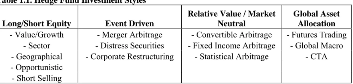
In case there is any position remaining at the end of the trading period, the position is closed at the prices of the last trading day without any comparison of the condition of deviation and the threshold level or inspecting whether the position is in profit or loss. Figure 3.1 illustrates the pairs trading strategy using two sample stocks. The top two lines are the normalized price series of the two stocks and the bottom line is the state of the position. Number of standard deviations for the threshold level is 2.0 in the sample illustration of the strategy.
Figure 3.1. Sample Pairs Trading Strategy
0,0 0,5 1,0 1,5 2,0 0 20 40 60 80 100 120 140 160 180 200
Trading Period Day Stock X Stock Y Stock X short Stock Y long Stock X long Stock Y short No position
We start to look for a trade signal and the first trade signal is detected at day 1 of the trading period. The deviation between the normalized prices is 0.507 while the standard deviation for the formation period is 0.123 and the threshold deviation level is 0.246. Stock X is sold and stock Y is bought with the expectation that the deviation will disappear in the future. On day 69 of the trading period, deviation crosses zero, which means the normalized prices of the two stocks become equal. The reverse of the first transactions are executed and stock X is bought back and stock Y is sold and position is closed.
On day 178, the deviation between the normalized prices becomes -0.324, which is lower than -2.0 standard deviation threshold level. This time, stock X is bought and stock Y is sold. 8 days later, on day 186, deviation between the normalized prices of the two stocks crosses zero. The reverse of the first transactions are executed and stock X is sold and stock Y is bought back and position is closed.
The ratio of number of stocks to be bought and sold (Nx,y,t) with the trade signal is
determined by the inverse ratio of the prices of the two stocks which is calculated as:
t x t y t y x P P N , , , , =
where Px,t is the price of stock X and Py,t is the price of stock Y at t. Using the ratio Nx,y,t makes the value of the investment in stock X and stock Y equal to each other and the position becomes dollar-neutral.
The trading rule we implemented is very simple. We open a long/short position when we detect divergence of the pair prices by a predetermined level. We close the position when the prices revert. As can be observed in the illustration, we do not have any assumption about the direction of the price movement. Therefore, position taken on the stocks is not on the same direction every time.
3.3. Return Calculation
The portfolios of pairs trading are formed by buying one stock and selling the other. Since the values of the investments are same, which means the strategy is dollar neutral; the return over the portfolio is not really the return over the capital invested. The performance of the strategy is calculated as the return over the value of one side of the transaction. Therefore, it is not possible to compare the performance of the pairs trading strategy with a buy and hold strategy, which requires capital to purchase one stock.
The performance of the strategy is considered according to the sum of the returns over the stock bought and sold during the trading period. First, we calculate return over each stock position separately as follows:
1 , , , = − n x o n x c n x P P R and 1 , , , = − n y o n y c n y P P R
In the equation, is the position opening price, is the position closing price of X
for the nth transaction and is the position opening price, is the position closing
price of X for the nth transaction.
n x o P , Pcx,n n y o P , Pcy,n
The total return for the pairs is calculated as:
(
)
∑
+ = n xn yn y x R R R 1 , , ,Since the positions are opened when the normalized price deviations are more than the threshold level and closed when the deviation is zero, any position that is closed before the last day of the trading period will result in profit, whether one of the stocks generates loss. Therefore, the condition of having negative return is only possible when the position is still open at the last day of trading period.
If the position is held on the last day of the trading period, the stock previously bought will be sold. The other stock, on the other hand, will be bought back and the position will be closed at the prices of the last trading day. Since it is possible to have a higher deviation than the threshold level while closing the position, we can encounter loss in one or both stock positions.
3.4. When does the Strategy Win or Fail?
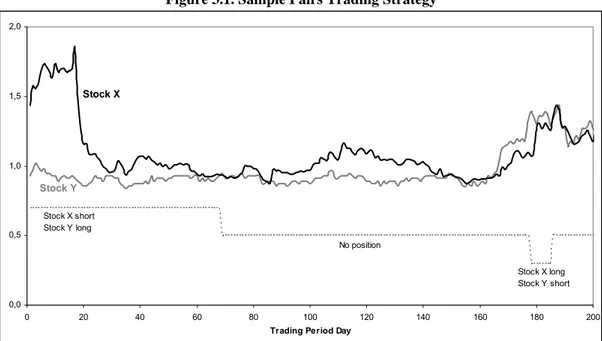
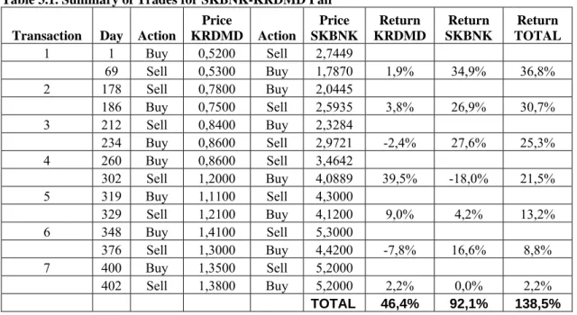
In this part of our study, we analyze two sample pairs, SKBNK-KRDMD and SKBNK- ARCLK. These two sample pairs have low deviations between the stock price series and they are expected to have good performance with the pairs trading strategy.
As shown in Figure 3.2, normalized prices of SKBNK and KRDMD move close to each other during the trading period. Although there is a significant comovement between the normalized price series, they sometimes deviate from each other and provide the trader with the opportunities to trade. The pairs provide 7 trade alternatives during the trading period, which is formed by selling SKBNK and buying KRDMD, or vice versa.
Figure 3.2. Sample Pairs Trading Strategy for SKBNK-KRDMD Pair
0,0 0,5 1,0 1,5 2,0 2,5 3,0 0 50 100 150 200 250 300 350 400
Trading Period Day SKBNK KRDMD SKBNK short KRDMD long SKBNK long KRDMD short No position
The details of the transactions are summarized in Table 3.1, which also includes the level of returns over the stocks for each transaction. In 4 of the transactions, the stocks bought gains value and the stock sold loses value and, as a result, both of the stocks return profits. In 3 of the transactions, one of the stocks results in positive return. The other stock, on the other hand, results in loss. However, the total return over the two positions is still positive as the profit level is higher than the loss. At the end of the trading period, the pair has 138.5% total return over 7 transactions.
Table 3.1. Summary of Trades for SKBNK-KRDMD Pair Transaction Day Action
Price KRDMD Action Price SKBNK Return KRDMD Return SKBNK Return TOTAL 1 1 Buy 0,5200 Sell 2,7449 0,0% 0,0% 0,0% 69 Sell 0,5300 Buy 1,7870 1,9% 34,9% 36,8% 2 178 Sell 0,7800 Buy 2,0445 0,0% 0,0% 0,0% 186 Buy 0,7500 Sell 2,5935 3,8% 26,9% 30,7% 3 212 Sell 0,8400 Buy 2,3284 0,0% 0,0% 0,0% 234 Buy 0,8600 Sell 2,9721 -2,4% 27,6% 25,3% 4 260 Buy 0,8600 Sell 3,4642 0,0% 0,0% 0,0% 302 Sell 1,2000 Buy 4,0889 39,5% -18,0% 21,5% 5 319 Buy 1,1100 Sell 4,3000 0,0% 0,0% 0,0% 329 Sell 1,2100 Buy 4,1200 9,0% 4,2% 13,2% 6 348 Buy 1,4100 Sell 5,3000 0,0% 0,0% 0,0% 376 Sell 1,3000 Buy 4,4200 -7,8% 16,6% 8,8% 7 400 Buy 1,3500 Sell 5,2000 0,0% 0,0% 402 Sell 1,3800 Buy 5,2000 2,2% 0,0% 2,2% TOTAL 46,4% 92,1% 138,5%
As the two stocks have a close comovement relationship and this relationship does not break down permanently during the trading period, the strategy formed with SKBNK and KRDMD is a good example for pairs trading with high return. In addition, having several number of trades executed and closed improves the performance of the pair as any position that is closed during the period results profit.
For the second sample pair, SKBNK and ARCLK, the normalized price series have two separate periods with different relationship characteristics. During the first half of the trading period, the price series move very closely to each other and deviate for short
periods. These short period deviations provide two transaction alternatives and both of these positions are formed by selling SKBNK and buying ARCLK.
However, during the second half of the trading period, the deviation between the normalized price series increases steadily and does not revert back. While normalized price series of SKBNK goes higher from the reference point, which is the first day of the formation period, normalized price series of ARCLK reverts to its mean and does not follow the upward move of SKBNK.
The reason for such a break down of the relationship can be fundamental which is due to a firm or sector specific news. Or, it can be only a directional movement of stock prices which can result from difference in transaction volumes of the stocks.
Figure 3.3. Sample Pairs Trading Strategy for SKBNK-ARCLK Pair
0,0 0,5 1,0 1,5 2,0 2,5 3,0 0 50 100 150 200 250 300 350 400
Trading Period Day SKBNK
ARCLK
SKBNK short ARCLK long
No position
Although, first two transactions result in a loss for ARCLK, the profit generated by buying SKBNK outperforms these losses and the pairs have returns of 25.6% and 19.4%. In the 3rd transaction, on day 181 of the trading period, the spread between the normalized price series crosses the threshold level, SKBNK is bought and ARCLK is sold. Since the
deviation after the entrance of the position does not revert back and reach to zero, the position can not be closed until the last day of the trading period. The position is closed at the last day without comparison of the condition of deviation and the threshold level. As a result, final transaction ends in losses of 20.15 and 108.1% for ARCLK and SKBNK, respectively.
Table 3.2 summarizes the transactions with SKBNK and ARCLK pair and the returns over these transactions.
Table 3.2. Summary of Trades for SKBNK-ARCLK Pair Transaction Day Action
Price ARCLK Action Price SKBNK Return ARCLK Return SKBNK Return TOTAL 1 1 Buy 9,8000 Sell 2,7449 0,0% 0,0% 0,0% 29 Sell 9,0000 Buy 1,8173 -8,2% 33,8% 25,6% 2 112 Buy 8,8500 Sell 2,2338 0,0% 0,0% 0,0% 155 Sell 8,3500 Buy 1,6734 -5,6% 25,1% 19,4% 3 181 Buy 10,2000 Sell 2,4988 0,0% 0,0% 0,0% 402 Sell 8,1500 Buy 5,2000 -20,1% -108,1% -128,2% TOTAL -33,9% -49,2% -83,1%
As mentioned above, pairs trading strategy results in profit in case the stock prices deviate form each other for short periods and revert back until the end of the trading period. As long as the stocks have a close price relationship and this relationship does not break down during the trading period, the strategy will be successful in detecting the deviations and profit generating transactions will be executed accordingly.
However, if the relationship between the price series changes significantly during the trading period, the strategy may end in loss as any position that is open at the end of the trading period should be closed.
4. EMPIRICAL RESULTS
In this part of our study, we build the results for the pairs trading strategy. We compare the performance of the strategy for different standard deviation threshold levels and summarize general trading settings such as the number of trades and the number of days in position. Since the assumption of having no transaction costs is not realistic for the strategy, we also analyzed the performance of the strategy after adding the transaction costs. In addition, to simulate the real market conditions as much as possible, we replicate our study with bid and ask prices that will be faced in case of a real transaction. Finally, we simulate a liquidity crisis scenario which uses the daily low and high prices for each stock which can form an idea about what can be the worst condition with the pairs trading strategy.
4.1. Strategy Performance
As the pairs trading strategy aims to gain profit over the relationship between the pair stocks price series, the performance of the strategy is evaluated according to the value added with each transaction. Therefore, the main determinant of good performance is the level of positive return achieved with the pairs trading strategy.
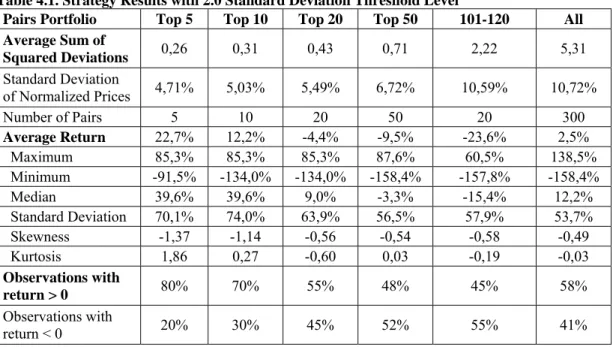
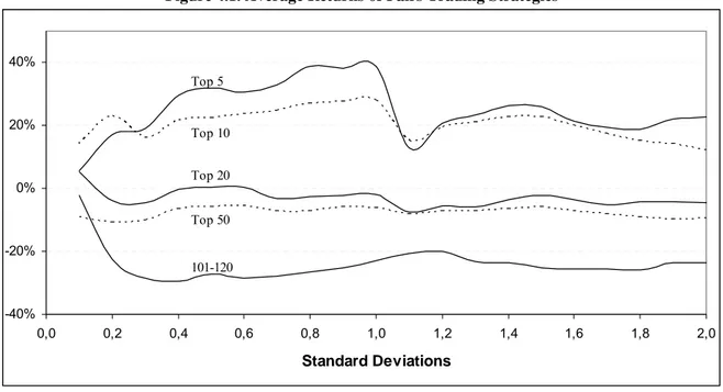
Table 4.1 summarizes the results for the trading period with 2.0 standard deviation threshold level. The results are categorized in 6 groups those composed according to the characteristics of the pairs in terms of sum of squared deviation levels between the normalized price series. While 4 groups consist of top 5, 10, 20 and 50 pairs with the lowest sum of squared deviation ranking, the 5th group has the pairs between 101st and 120th ranking. The last portfolio includes all possible pair alternatives that can be formed with the sample set.
Average return levels show that pairs trading strategy that invests in top 5 pairs earn 22.7% per pair on average during the trading period. In case the number of pairs included in the