In this paper, a supervised algorithm for the evaluation of geophysical sites using a multi-level cellular neural network (ML-CNN) is introduced, developed, and applied to real data. ML-CNN is a stochastic image processing technique based on template optimization using neighborhood relationships of the pixels. The separation/enhancement and border detection performance of the proposed method is evaluated by various interesting real applications. A genetic algorithm is used in the optimization of CNN templates. The first application is concerned with the separation of potential field data of the Dumluca chromite region, which is one of the rich reserves of Turkey; in this context, the classical approach to the gravity anomaly separation method is one of the main problems in geophysics. The other application is the border detection of archeological ruins of the Hittite Empire in Turkey. The Hittite civilization sites located at the Sivas-Altinyayla region of Turkey are among the most important archeological sites in history, one reason among others being that written documentation was first produced by this civilization.
Keywords: Cellular neural networks (CNN), genetic algorithm, data processing, information retrieval, potential anomaly separation, archeo-geophysics.
Manuscript received June 29, 2004; revised Feb. 11, 2005.
Erdem Bilgili (phone: +90 262 6538490, email: [email protected] ) is with the Department of Electrical Engineering, Gebze High Technology Institute, Turkey.
I. Cem Göknar (email: [email protected]) is with the Department of Electronics and Communications Engineering, DOGUS University, Turkey.
Ali Muhittin Albora (email : [email protected]) is with the Department of Geophysics Engineering, Istanbul University , Turkey.
Osman Nuri Uçan (email: [email protected]) is with the Department of Electrical and Electronics Engineering, Istanbul University, Turkey.
I. Introduction
Potential-field maps usually contain a number of anomalies that are superimposed onto each other. For instance, a magnetic map may be composed of regional, local, and micro-anomalies. In this case, the determination of the causative sources’ boundaries suffers from nearby source interferences, thus yielding mislocations. Since one type of anomaly often masks another, the need arises to separate the various anomalies from each other.
Potential data observed in geophysical surveys are the sum of related fields produced by all underground sources. The targets for specific surveys are often small-scale structures buried at shallow depths, and these targets are embedded in a regional field that arises from sources that are usually larger and deeper than the targets or are located farther away. Moreover, the change in the potential field of residual anomalies is much quicker than the corresponding change in the potential field of regional anomalies. Correct estimation and removal of the regional field from initial field observations
yields the residual field produced by the target sources.
Interpretation and numerical modeling are carried out on the residual field data, and the reliability of the interpretation depends to a great extent upon the success of the regional-residual separation using the distinguishing properties mentioned in this paragraph.
Interpretation of magnetic and gravity anomalies makes extensive use of enhanced maps as an initial step to eliminate or attenuate unwanted field components in order to isolate the desired anomaly (e.g., residual-regional separations).
Potential Anomaly Separation and Archeological
Site
Localization Using Genetically Trained
Multi-level
Cellular Neural Networks
Frequency analyses of gravity and magnetic anomalies were carried out in 1958 and vertical derivatives of contours were obtained [1]. Then, for the interpretation of magnetic fields, a two dimensional (2-D) harmonic analysis was performed in 1965 [2]. 2-D filters were employed by interpolating data stored on pixels of a square grid [3], [4] using Hankel transformations [5] and through Fourier transform techniques [6]. A digital filter using Hankel transformations is given in [7]. Important observations, based on the density contrast of the Mississippian-Pennsylvanian interface, were made by separation of regional anomalies from the residual ones using Wiener filtering techniques [8]. Applications of linear filters and Werner de-convolution algorithms are given in [9]. An equally important problem, for which a method is given in [10], is the determination of boundaries between different structures of buried bodies. The use of wavelets are explored in: i) separation of regional and residual anomalies of potential fields [11], [12], ii) evaluation of aeromagnetic data in [13], iii) modeling the geometry of geological bodies using multi-scale edge analysis [14], and iv) de-noising of signals from potential field effects and estimating borders of the buried objects [15]-[17]. In this paper, a supervised algorithm for a multi-level cellular neural network (ML-CNN) is developed and applied to real data obtained from the Dumluca iron site and archeological ruins of the Hittite Empire in Turkey.
In the first part of section II, the CNN structure is explained and the multi-level approach is introduced. In the second part, genetic operations and the cost function used in the paper are defined; the algorithm used for the applications considered in this paper is then presented.
Section III is concerned with the application of ML-CNN as follows: First, the CNN is trained with input-desired output (target image) data pairs, tested with synthetic examples, and then applied to real data. The best chromosomes and the related CNN templates obtained from the algorithm are given; raw data maps and the ensuing processed maps that clearly show the improvement are also exhibited.
Section IV concludes the paper by exploring some future applications.
II. Multi-level Cellular Neural Network
1. Basic CNN Structure
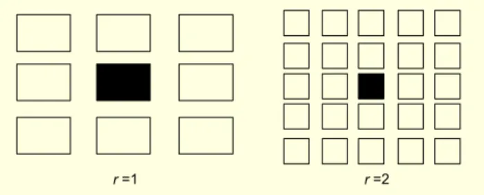
A basic 2-D CNN can be viewed as an array of basic processing units as shown in Fig. 1.
In a conventional artificial neural network (ANN), all cells communicate with each other, whereas in CNN, only cells within a prescribed neighborhood do so. The r-neighborhood of cell Ci,j is defined [18] as Nr(i,j) = {C(k,l)|max{|k - i|,|l - j|}≤r,
Fig. 1. 1- and 2-neighborhoods of the central cell.
r =1 r =2
Fig. 2. A typical circuit cell (i,j). + - Eij Iij C R x Ixu(i,j;k,l) Ixy(i,j;k,l) Iyx Ry yij + + Ixu(i,j;k,l)=B(i,j;k,l)uij Ixy(i,j;k,l)=A(i,j;k,l)yij Iyx=(|xij+1|-|xij-1|)/2Ry xij
1≤k≤M; 1≤l≤N} and shown in Fig.1 for r=1 and r=2. As
each cell communicates with its neighbors, the effect of a cell propagates to cells farther away than r. Figure 2 shows a possible equivalent circuit of a single cell as given in [18] where all elements are linear with the sole exception of the dependent current source Iyx defined via the piecewise linear
sigmoid given in Fig. 3.
In Fig. 2, uij, xij, and yij show respectively the input, capacitor,
and output voltages, and Iij is the independent bias current
source; dependent source coefficients A(i,j;k,l) and B(i,j;k,l) reflect respectively the weighted effects of the output and input of cell (k,l) in the considered neighborhood, on cell (i,j) (these coefficients will be the elements of the template matrices A and
B). Assuming normalized element values (CRx=1) and a
space-invariant CNN, namely that A(i,j;k,l)= A(i-j,k-l) and B(i,j;k,l)=
B(i-j;k-l), Kirchoff’s current law written in terms of node
voltage xij yields the following state equation of the cell:
. ,..., 2 , 1 , ,..., 2 , 1 for , ) ( u ) ( ) ( ) ( 1 2 1 1 2 1 1, 1 1 2 1 1 2 1 1, 1 n j m i ij r k r l kl i k r j l r r k r l kl i k r j l r ij ij I t B t y A t x dt t dx = = + ∑ ∑ + ∑ ∑ + − = + = + = + −− +−− + = + = +−− +−− (1) The following advantages of assuming a restricted neighborhood and space-invariance are huge:
i) the natural assignment of double indexed variables and weight coefficients to matrices yields a very compact 2-D convolution representation as in (2),
two simple matrices (of size 3 × 3 for r=1 and 5 × 5 for r=2) called cloning templates, or templates in short, and
iii) this small size of the templates, by reducing the number of network parameters to be found, becomes especially useful in the design of a CNN that performs specific tasks in image processing among other subjects; as most design procedures use optimization techniques where the optimization variables are template matrix elements, this number reduction becomes of crucial importance. The same goes for genetic algorithms and this will soon be appreciated in subsection II.3.
2. Multi-level CNN
The cellular neural networks (CNN) introduced above have a well-suited structure for image processing. Their normalized differential state equations, which are nothing but a compact matrix representation of (1), can be described via the matrix convolution operator by
X A Y B U I dt
dX =− + × + × + , (2)
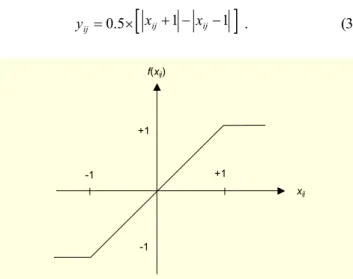
where U, X, Y are the M×N input, state, and output matrices; A and B represent the feedback and feed-forward connections, respectively; and I is an M×N offset matrix representing the bias currents. The relationship between the state and the output of cell ij shown in Fig.3 is the nonlinear function
[
1 1]
5 . 0 × + − − = ij ij ij x x y . (3)Fig. 3. Piecewise linear sigmoid function
f(xij) xij -1 +1 +1 -1
According to (2), CNN output changes until the derivative of the state variable of the CNN is zero; so, the last stable output is defined as ij ij Y Y∞ = , when =0 dt dX for all t.
For designing a stable CNN, A and B should be symmetrical and A22 must be greater than one, if the size of A has been
selected as 3×3. CNNs are used for different special signal/image processing applications with various templates. The multi-level CNN introduced in this paper consists of the serial cascaded connection of similar type CNN structures. The same templates are used in each level, and the output of each CNN level is the input of the next CNN level in the cascade connection.
3. Genetic Algorithms
Genetic algorithms are based on the mechanisms of natural selection and genetics and have proven to be effective in a number of applications. They work with a binary coding of the parameter set and search from a number of points of the parameter space for the best one; they use only a cost function during the optimization and do not need derivatives of the cost function or other information. In genetic algorithms, reproduction and mutations may cause the chromosomes of children to be different from those of their biological parents, and crossing-over processes create different chromosomes of children by interchanging some parts of the parent chromosomes. Like in nature, the genetic approach solves the problem of finding good chromosomes by manipulating the chromosomes blindly without any knowledge about the problem they aretrying to solve [19]-[21]. A general outline of the genetic approach used in this paper is presented next.
Step 1. Construction of the initial population. A matrix called
a population matrix is constructed. Each row of the population matrix represents chromosomes and each column represents the bits in chromosomes, and its size is m×n. At the beginning, this matrix is constructed randomly.
Step 2. Extraction of the CNN templates. Chromosomes
represent the binary codes of the elements of the CNN templates, A, B, I. In this step, each chromosome is decoded and the elements of the CNN are computed in a chosen interval. Since templates A and B contain two entries each, the center ones a22 , b22 and a11 , b11 representing all other equal template
elements, the total number of elements becomes five including the value for I. These elements are shown in vector form as
S = [a11, a22, b11, b22, I]. (4)
Each of the elements of S being coded in binary, the chromosome S0 used in the algorithm is obtained from S as
follows: The first five bits in S0 represent the first five bits of the
template elements, the second five bits represent the second five bits of the template elements in each chromosome, and so on; the length of each chromosome will be denoted by LengthS.
chromosome. In this step, an image that was selected as the
training image is fed as input to the CNN, which works with the templates belonging to the first chromosome. After the CNN output appears to be stable, the cost function is computed between this output image and the desired target image. This process is repeated with the template sets belonging to each chromosome in the population. The cost function has been selected in this study as follows:
(
)
ij M i N j j i T P I B A, , , , cost =∑∑
⊕ , (5)where P and T represent the CNN output image and the target
image, respectively, and the symbol ⊕ stands for the XOR
operation between respective elements (pixels) of P and T. After finding the cost function, the associated fitness function is evaluated for each chromosome according to the rule,
) , , cost( ) , , (A B I M N A B I fitness = × − . (6)
Another rule has been defined for the stopping criterion as
N M n
stcriterio =0.99× × . (7) If the maximum fitness value of the chromosome is greater than the stopping criterion, the algorithm is stopped and the chromosome whose fitness value is the maximum in the population is selected. The templates, which have been extracted from this selected chromosome, are the most proper templates that satisfy the task desired to be realized.
Step 4. Creation of a new generation. Before creating the
next generation, fitness values of the population are sorted in descending order and normalized relative to the sum of the fitness values of the population. A random number r between 0 and 1 is generated. Then, the first population member is selected whose normalized fitness, added to the normalized fitness of the preceding population members, is greater than or equal to r. This operation is repeated several times and any chromosome whose fitness is bad is deleted from the population. This above procedure is called reproduction in genetic algorithms. The reproduction process does not generate new chromosomes, but rather elects the best chromosomes in a population and increases the number of chromosomes whose fitness values are relatively greater than the others. After the reproduction, depending on the application, K pairs of chromosomes are selected as parents randomly. Two numbers
s1, and s2 between 1 and the length of chromosomes are
generated. The bit strings between s1 and s2 are called the
crossover site. During the crossing-over process, bit strings in the crossover sites in each pair of chromosomes are
interchanged and two new chromosomes are created from a pair of old chromosomes. At last, 2K new chromosomes, which are called children, are generated to build the new population. Over these chromosomes, the mutation operation is carried-out. Since the mutation probability has been set to 1%, 0.01×m×n bits are selected randomly from the population and inverted. The chromosome whose fitness value was the best before the reproduction process is added and another randomly selected chromosome is deleted form the final generation; the purpose of this addition is to preserve the fittest chromosome of the previous step; this new population is the next generation population. After obtaining the new generation, the search procedure goes to the second step and continues until the stopping criterion is met.
III. ML-CNN Applications on Synthetic and Real Data
Various applications of ML-CNN have been considered and the performance of the proposed approach has been evaluated. The first example is on the evaluation of the separation of potential anomalies. The other example is on the border detection property of ML-CNN. The numerical values used in the steps of the algorithm given in section II.3 are listed in Tables 2 and 5. It should be observed that for general templates
A, B, I, LengthS = [2(2r+1)2+1]k, where r is the neighborhood
considered in the CNN, and k is the precision (number of bits) of each template element. For r=1 and k=16, LengthS=304 for general templates, whereas it reduces to
LengthS=(2+2+1)16=80 for templates considered in this paper.
1. For Magnetic Data
Figure 4 shows the location and physical attributes of a dipole that will be used to calculate the vertical magnetic field
Z at the point P caused by this dipole; these calculations are
done using (8).
Z = (Vertical component of field due to –m)
– (Vertical component of field due to +m)
( )
(
)
{
3}
2 3 1 0S z/r z Lsin /r kF − + α = , (8)where k is the susceptibility, F0 is the earth’s total field, z is the
average depth of the dipole, S is the surface,and the vertical field being positive downward; other parameters are defined in Fig. 4.
A. Training CNN for Gravitational Data
In order to cover the most difficult separation problem, two dipoles different in size and location as described in Table 1
Fig. 4. Synthetic dipole model. L +m -m r1 r2 P z x Surface θ1 θ2 β α
Table 1. Parameters of two dipoles having the same (x,y) coordinates
Parameters Dipole 1 Dipole 2 (x,y) coordinates (32,32) (32,32)
Z (dip) 5 25 L (along) 8 30
α(angle) 90 90
Fig. 5. Synthetic example for training procedure of magnetic
data: 2 dipoles having the same (x,y) coordinates with properties as in Table 1: (a) regional anomaly of dipole 2 (contour interval 0.008 nT) (b) residual anomaly of dipole 1 (contour interval 0.4 nT) (c) total vertical magnetic anomaly of 2 dipoles (contour interval 0.2 nT) (d) ML-CNN output (contour interval 0.04 nT).
10 20 30 40 60 80 10 20 30 40 60 80 10 20 30 40 60 80 10 20 30 40 60 80 10 20 30 40 60 80 10 20 30 40 60 80 10 20 30 40 60 80 10 20 30 40 60 80 0.123 0.107 0.075 0.059 0.043 0.027 0.011 -0.005 0.091 3.4 3.0 2.2 1.8 1.4 2.6 1.0 0.6 0.2 -0.2 (a) (b) 3.4 3.0 2.2 1.8 1.4 1.0 0.6 -0.2 2.6 0.2 -0.73 -0.77 -0.85 -0.89 -0.81 -0.93 -0.97 -1.01 (c) (d) nT nT nT
constitute the first synthetic example; the main reason for selecting this configuration being that when using magnetic
data it is relatively very difficult to separate structures lying one on top of the other.
The effect of the larger dipole 2, creating the regional anomaly, covers the residual effects of the smaller dipole 1 and thus makes its detection difficult from raw data. The vertical magnetic anomaly map of these two dipoles, with the same x, y but with different z coordinates, will be evaluated. The approach used for determining CNN templates is as follows:
i) total vertical magnetic field, with both dipoles present, is calculated from (8) providing the training input data,
ii) using (8), the vertical magnetic field of the small dipole closer to the surface is calculated giving the desired output, and
iii) genetic training is applied to data obtained in i) and ii), and the templates A, B, I are obtained.
The regional and residual anomalies and their sum total vertical anomaly map are drawn in Figs. 5(a) through 5(c), using (8) and the properties in Table 1. The total vertical anomaly and residual anomaly maps are taken as input and desired output, respectively. At the end of the training process, genetic algorithm parameters were obtained as in Table 2.
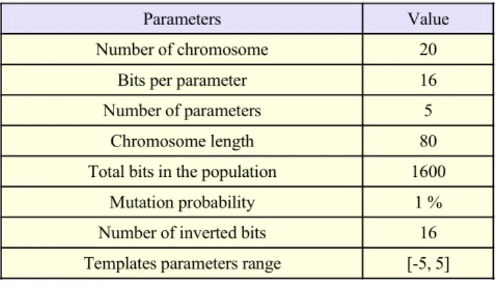
Table 2. Genetic training algorithm parameters for magnetic data.
Parameters Value Number of chromosome 20
Bits per parameter 16 Number of parameters 5
Chromosome length 80 Total bits in the population 1600
Mutation probability 1 % Number of inverted bits 16 Templates parameters range [-5, 5]
The best chromosome and the following templates were found after the 108 generations:
01001111], 1110011100 0100100011 0100001000 000 0000110001 1000010000 1000010010 [101000001 BC= 0.371. , 1.0032 1.0032 1.0032 1.0032 3.7542 1.0032 1.0032 1.0032 1.0032 , 0.0020 0.0020 0.0020 0.0020 0.5015 0.0020 0.0020 0.0020 0.0020 = ⎥ ⎥ ⎥ ⎦ ⎤ ⎢ ⎢ ⎢ ⎣ ⎡ = ⎥ ⎥ ⎥ ⎦ ⎤ ⎢ ⎢ ⎢ ⎣ ⎡ = I B A (9)
Figure 5 shows that residual/regional anomalies are satisfactorily separated by the genetically trained ML-CNN approach.
B. ML-CNN Applications to Synthetic Examples
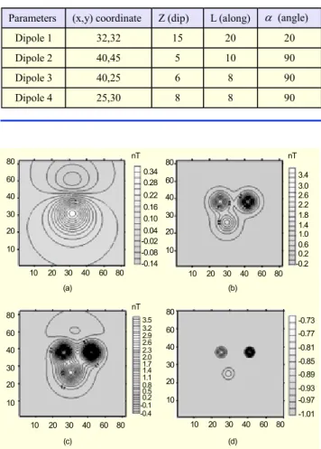
The multi-level CNN with templates obtained as in (9) was applied to magnetic data of the synthetic example consisting of four dipoles with properties described in Table 3; the magnetic map corresponding to the raw data of Table 3 is shown in Fig. 6(c) and that of CNN output data in Fig. 6(d).
Table 3. Synthetic magnetic data with 4 dipoles.
Parameters (x,y) coordinate Z (dip) L (along) α (angle) Dipole 1 32,32 15 20 20 Dipole 2 40,45 5 10 90 Dipole 3 40,25 6 8 90 Dipole 4 25,30 8 8 90
Fig. 6. A synthetic example for testing procedure of magnetic
data: vertical magnetic field of 4 dipoles having different (x,y) coordinates with properties as in Table 3: (a) regional anomaly (contour interval 0.03 nT), (b) residual anomaly (contour interval 0.2 nT), (c) total vertical magnetic anomaly of 4 dipoles (contour interval 0.1 nT), and (d) ML-CNN output (contour interval 0.02 nT).
10 20 30 40 60 80 10 20 30 40 60 80 10 20 30 40 60 80 10 20 30 40 60 80 10 20 30 40 60 80 10 20 30 40 60 80 10 20 30 40 60 80 10 20 30 40 60 80 0.34 0.28 0.16 0.10 0.04 -0.02 -0.08 0.22 3.4 3.0 2.2 1.8 1.4 2.6 1.0 0.6 0.2 (a) (b) 3.5 3.2 2.6 2.3 2.0 1.7 1.4 0.8 2.9 1.1 -0.73 -0.77 -0.85 -0.89 -0.81 -0.93 -0.97 (c) (d) 0.5 -0.10.2 nT nT nT -0.14 -0.2 -1.01 -0.4
C. Detection of Hittite Empire Walls with ML-CNN
The Hittite civilization has been investigated since1966 by archeologists such as A. Muller and geophysicists like H.
Stumpel [22], [23].
The magnetic anomaly map of the ruins of the Hittite Empire is shown in Fig. 7(a), and data obtained from Fig. 7(a) is taken as initial data and applied to CNN as input as well as the initial state. In the following, ML-CNN results shown in Figs. 7(c) through 7(d) are compared with the results of the classical Halck’s second vertical-derivative-based approach shown in Fig. 7(b). It is clearly observed that ML-CNN has much better separated potential anomalies, as compared to the classical deterministic methods. The real data can also be evaluated by altering multi-level process parameters, a feature that is not available with the classical methods. It has been observed that as the level number is increased, the ML-CNN’s output separates the dominant factors of the real data. The precise information about the location of the buried walls of the Hittite civilization in the Sivas-Altinyayla region of Turkey has been obtained and is exhibited with Figs. 7(c) and 7(d) in the paper and compared with those of the other methods.
Fig. 7. Treatment of data from ruins of the Hittite Empire: (a)
magnetic anomaly map of ruins of the Hittite Empire, (b) Halck’s second vertical derivative approach output for real data, (c) ML-CNN output for real data of the Hittite Empire, and (d) three-level ML-CNN output.
(a) (b) (c) (d) N N N N Scale meter 0 5 10 595 590 585 580 575 570 565 560 555 320 325 330335340 345350355 360 365 595 590 585 580 575 570 565 560 555 320 325 330 335 340 345 350355 360 365 595 590 585 580 575 570 565 560 555 320 325 330335340 345350355 360 365 595 590 585 580 575 570 565 560 555 320 325 330 335 340 345 350355 360 365
2. For Gravitational Data
The second application to potential anomaly separation is the classification of raw gravitational data using ML-CNN. The following formula is used to calculate the gravity effects of a buried sphere at any point P on the earth’s surface:
2 02 2 32 ) (x y h h m k G + + = with π 3ρ 3 4 r m= , (10) where k0 =6.67×10⁻⁸ cm3gr-1s-2 is the gravitational constant, r
the radius of the sphere ρ , the density of the sphere, h the depth of the sphere’s center, x and y the coordinates of P measured with the origin being the projection of the sphere’s center to the surface, and G the value of the gravity anomaly. Figure 8 shows the change in the gravity anomaly with respect to distance in the x direction.
A. Training CNN for Gravitational Data
Three spheres with different sizes, densities, and coordinates as described in Table 4 have been used for training an ML-CNN. The sphere placed at the deepest location disturbs the gravity anomaly effects of the sphere closer to the surface. Genetic algorithm parameters are shown in Table 5. Figure 9(c) depicts the input data and Fig. 9(b) the desired output data.
Training based on these data resulted in the following best chromosome and templates after 403 generations:
100101] 1000010010 1001011010 1101101000 10000 1000000010 1100101001 1101101011 [000101011 BC= . 64 . 2 , 9153 . 0 9153 . 0 9153 . 0 9153 . 0 7656 . 7 9153 . 0 9153 . 0 9153 . 0 9153 . 0 , 2246 . 0 2246 . 0 2246 . 0 2246 . 0 5000 . 0 2246 . 0 2246 . 0 2246 . 0 2246 . 0 − = ⎥ ⎥ ⎥ ⎦ ⎤ ⎢ ⎢ ⎢ ⎣ ⎡ − − − − − − − − = ⎥ ⎥ ⎥ ⎦ ⎤ ⎢ ⎢ ⎢ ⎣ ⎡ − − − − − − − − = I B A (11) As clearly indicated by Fig. 9, very good separation is achieved by using the ML-CNN approach.
Fig. 8. Synthetic sphere model
0 80mGal h r 0 x P(x) 40 0 km 10 20 30
Table 4. Gravity model with 3 spheres.
Parameters (x,y) coordinates h (depth) r (radius) ρ (density) sphere 1 31,31 10 6 1 sphere 2 46,51 3 2 13 sphere 3 16,16 4 2 1.2
Table 5. Genetic algorithm training parameters for gravitational data.
Parameters Value Number of chromosome 30
Bits per parameter 16 Number of parameters 5
Chromosome length 2400 Total bits in the population 1600 Mutation probability 1% Number of inverted bits 24 Templates parameters range [-8, 8]
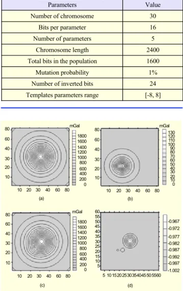
Fig. 9. A synthetic example of three spheres with properties in
Table 4 for training gravitational data: (a) regional anomaly field (contour interval 100 mGal), (b) residual anomaly map (contour interval 10 mGal), (c) total gravity anomaly field (contour interval 100 mGal), and (d) ML-CNN output (contour interval 0.005 mGal).
10 20 30 40 60 80 10 20 30 40 60 80 10 20 30 40 60 80 10 20 30 40 60 80 10 20 30 40 60 80 10 20 30 40 60 80 35 40 4550 55 60 5 10 15 30 5055 1800 1600 1200 1000 800 600 400 200 1400 130 120 100 80 70 110 50 40 30 10 (a) (b) -0.967 -0.972 -0.982 -0.987 -0.977 -0.992 -0.997 (c) (d) 90 60 20 1800 1600 1400 1200 1000 800 600 400 200 0 30 25 20 15 10 5 20 25 35 40 45 mGal mGal -1.002 0 0 60 mGal
B. ML-CNN Applications to Synthetic Examples
The ML-CNN with templates obtained in part A of this section was applied to the gravitational data of the synthetic
example consisting of four spheres with properties described as in Table 6; the measured potential anomaly map corresponding to the raw data of Table 6 is shown in Fig. 10(c) and that of ML-CNN output data in Fig. 10(d).
Table 6. Synthetic gravity data with 4 spheres.
Parameters (x,y) coord. h (depth) r (radius) ρ (density) Sphere 1 31,31 20 10 1.2 Sphere 2 41,43 8 4 1 Sphere 3 18,44 6 3 0.9 Sphere 4 19,16 5 3 1.1
Fig. 10. The synthetic example of four spheres with properties
in Table 6 for testing ML-CNN for gravitational data: (a) regional anomaly field (contour interval 100 mGal), (b) residual anomaly map (contour interval 15 mGal), (c) bouguer anomaly field (contour interval 100 mGal), and (d) ML-CNN output (contour interval 0.003 mGal).
10 20 30 40 50 60 10 20 30 40 50 60 10 20 30 40 60 80 10 20 30 40 60 80 10 20 30 40 50 50 10 20 30 40 60 80 10 20 30 40 60 80 10 20 30 40 60 80 1700 1500 1100 900 700 500 300 100 1300 240 210 150 120 90 180 60 30 (a) (b) -0.980 -0.986 -0.989 -0.983 -0.992 -0.995 -1.001 (c) (d) -0.998 1700 1500 1100 900 700 500 300 1300 mGal 0 -0.977 mGal mGal 100
C. Analysis of Potential Anomaly Map of Dumluca Chromite Iron Ore Using ML-CNN
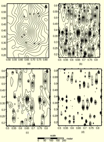
The gravity anomaly map of the Dumluca chromite ore around Divriği, Turkey is given in Fig 11(a); the real data corresponding to this map was applied to a multi-level CNN with templates obtained in part A of this section. Halck’s second vertical derivative approach is applied to Fig 11(a), and its outputs are shown in Figure 11(b), while CNN outputs are shown in Figs. 11(c) through 11(d). The studies on this region show that the coordinates of anomalies obtained using the ML-CNN approach conform with the iron ore concentration
regions reported in [24] in the sense that some minor concentrations were missed but there were no false detections.
Fig. 11. (a) Dumluca gravity anomaly map (contour interval is
0.2), (b) Halck’s second derivative approach output (contour interval is 0.01), (c) three level ML-CNN output (contour interval is 0.003), and (d) five level ML-CNN output (contour interval is 0.003).
0 50 100 150 200 meter scale 0.50 0.55 0.60 0.65 0.70 0.75 0.80 0.20 0.25 0.30 0.35 0.40 0.45 0.50 0.55 0.60 (a) (c) (d) (b) 0.5 0.55 0.6 0.65 0.7 0.75 0.8 0.2 0.25 0.3 0.35 0.4 0.45 0.5 0.55 0.6 0.5 0.55 0.6 0.65 0.7 0.75 0.8 0.2 0.25 0.3 0.35 0.4 0.45 0.5 0.55 0.6 0.5 0.55 0.6 0.65 0.7 0.75 0.8 0.2 0.25 0.3 0.35 0.4 0.45 0.5 0.55 0.6
IV. Conclusions
In this paper, multi-level cellular neural networks (ML-CNN) have been presented and used for evaluating geophysical data concerning potential anomaly separation and border detection. CNNs trained with synthetic data using genetic algorithms have been successfully applied in particular to the real data of two important geophysical sites in Turkey: the Dumluca chromite ore site and the Hittite ruins archeological site. The studies on Dumluca show that the coordinates of anomalies obtained using the ML-CNN approach conformed well with the iron ore concentration regions reported in [24] by MTA, the General Directorate of Research and Exploration. In particular, the residual separation of ML-CNN has provided satisfactory results; it has been observed that as the level number is increased ML-CNN better
separates the dominant factors of the real data and has a sharper separation and edge detection property than the classical derivative based methods.
Future research directions may include applications such as fault-line location and land-mine detection.
References
[1] W.C. Dean., “Frequency Analysis for Gravity and Magnetic Interpretation,” Geophysics, vol. 23, 1958, pp. 97-127.
[2] B.K. Bhattacharyya, “Two-Dimensional Harmonic Analysis as a Tool for Magnetic Interpretation” Geophysics, vol. 30, no. 5, Oct. 1965, pp.829-857.
[3] D. Fuller, “Two-Dimensional Frequency Analysis and Design of Grid Operators,” Mining Geophysics, vol. 2, 1967, pp. 658-708. [4] E.G. Zurflueh, “Applications of Two-Dimensional Linear
Wave-Length Filtering,” Geophysics, vol.32, no. 6, 1967, pp. 1015-1035. [5] P.M. Lavin and J. F. Devane, “Direct Design of Two-Dimensional
Digital Wavenumber Filters,” Geophysics, vol. 35, 1970, pp.1073-1078.
[6] W. G. Clement, “Basic Principles of Two-Dimensional Digital Filtering,” Geophysical Prospecting, vol. 21, 1973, pp. 125-145. [7] W. L. Anderson, “Computer Program Numerical Integration of
Related Hankel Transforms of Orders 0 and 1 by Adaptive Digital Filtering,” Geophysics, vol. 44, no. 7, 1979, pp. 1287-1305. [8] R.O. Hansen and R.S. Pawlowski, “Reduction to the Pole at Low
Latitudes by Wiener Filtering,” Geophysics, vol. 54, 1989, pp. 1607-1613.
[9] R.O. Hansen and M. Simmonds, “Multiple-Source Werner Deconvolution,” Geophysics, vol. 58, 1993, pp. 1792-1800. [10] R.J. Blakely and R.W. Simpson, “Approximating Edges of Source
Bodies from Magnetic or Gravity Anomalies,” Geophysics, vol. 51, no. 7, 1986, pp. 1494-1498.
[11] M. Fedi and T. Quarta “Wavelet Analysis for the Regional Residual and Local Separation of Potential Field Anomalies,”
Geophysical Prospecting, vol. 46, 1988, pp.507-525.
[12] P. Hornby, F. Boschetti, and F.G. Horowitz, “Analysis of Potential Field Data in the Wavelet Domain,” Geophysical J. International, vol. 137, 1999, pp. 175-196.
[13] T.A. Ridsdill-Smith and M.C. Dentith, “Wavelet Transform in Aeromagnetic Processing,” Geophysics, vol. 64, no. 4, 1999, pp. 1003-1013.
[14] D. Holden, N. Archibald, F. Boschetti, and M. Jessell, “Inferring Geological Structures Using Wavelet-Based Multiscale Edge Analysis and Forward Models,” Exploration Geophysics, vol. 31, 2000, pp. 617-621.
[15] F. Boschetti, P. Hornby, and F.G. Horowitz, “Wavelet Based Inversion of Gravity Data,” Exploration Geophysics, vol. 32, 20001, pp. 48-55.
[16] O.N. Ucan, B. Sen, A.M. Albora, and A. Özmen, “A New Gravity
Anomaly Separation Approach: Differential Markov Random Field (DMRF),” Electronic Geosciences, vol. 5, no. 1, 2000. [17] O.N. Ucan, S. Şeker, A. M. Albora, and A. Özmen, “Separation of
Magnetic Field Data Using 2-D Wavelet Approach,” J. Balkan
Geophysical Society, vol. 3, 2000, pp. 53-58.
[18] L.O. Chua and L. Yang, ‘‘Cellular Neural Networks: Theory,’’
IEEE Trans. on Circuit and Systems, vol.35, 1988, pp. 1257-1272.
[19] J.H. Holland, Adaptation in Neural and Artificial Systems, University of the Michigan Press, Ann Arbor, MI, 1975.
[20] T. Kozek, T. Roska, and L.O. Chua. ‘‘Genetic Algorithms for CNN Template Learning,’’ IEEE Trans. on Circuit and Systems, vol. 40, no. 6, 1988, pp. 392-402.
[21] L. Davis, Handbook of Genetic Algorithms, Van Nostrand Reinhold, New York, 1991.
[22] H. Stümpel, ‘‘Untersuchungen in Kusakli: Geophysikalische Prospektion,” Mitteilungen der Deutschen Orient-Geselschaft, Berlin, vol. 129, 1997, pp. 134-140.
[23] H. Stümpel, ‘‘Untersuchungen in Kusakli: Geophysikalische Prospektion,” Mitteilungen der Deutschen Orient-Geselschaft, Berlin, vol. 130, 1998, pp. 144-153.
[24] N. Yıldız, “Drilling Report of Divriği-Dumluca Iron Ore,” MTA Report, no. 315, Ankara, 1977.
Erdem Bilgili received the BS degree in
electronics and communication engineering from Yıldız Technical University (YTU), Turkey in 1996 and the MS degree in electronics engineering from Gebze Institute of Technology (GYTE), Turkey in 1999. He is currently a PhD student in electronics engineering, GYTE, Turkey. From 1998 to 2004, he worked for GYTE as a Research Assistant. From 2000 to 2004, he also worked for TUBITAK MAM as a Part-Time Researcher. Since 2004, he has been working for TUBITAK MAM. His research interests include the applications of neural networks, cellular neural networks, genetic algorithms, image processing, pattern recognition, microwave imaging techniques, microwave tomography, and geophysics.
I. Cem Göknar (F IEEE) was born in Istanbul,
Turkey. He received the B.Sc. and M. Sc. degrees from Istanbul Technical University and the Ph.D degree from Michigan State University in 1969. He received NATO’s Senior Scientist Grant and the Minna-James-Heineman-Stiftung Award and was a Visiting Professor at the Univ. of California at Berkeley, Univ. of Illinois, U-C, Univ. of Waterloo at Ontario, Canada and Technical University of Denmark at Lyngby. From 1995-1997 he served as European Circuit Society Council member. Currently, he is a professor, head of Electronics and Communications Engineering Department, Director of Science and Technology Institute at Doğuş University, Istanbul, Turkey, and IEEE-CAS Chapter Chair, Turkey Section. His research interests include nonlinear networks and systems, signal processing in general and neural networks and applications, interconnect modeling and simulation, and fast-timing simulators in particular.
Ali Muhittin Albora received the BS, MS and
PhD degrees in geophysics engineering from Istanbul University, Istanbul, Turkey, in 1985, 1992 and 1998. He was appointed as an Assistant Professor in 2001, and as an Associate Professor in 2003. Since 2003, he has been with Istanbul University, Engineering Faculty, Department of Applied Geophysics. His research interests include the use of potential field methods in the solution of regional and crustal geological problems, and the applications of computer techniques in geophysics.
Osman Nuri Uçan was born in Kars in January,
1960. He received the B.Sc., M.Sc. and PhD degrees in electronics and communication engineering from Istanbul Technical University (ITU) in 1985, 1988, and 1995. During 1986-1997 he worked as a Research Assistant at ITU and was a Supervisor at TUBITAK-Marmara Research Center in 1998. He is a Professor, Vice Dean of the Engineering Faculty, and Vice Chair of EE Engr. Dept., all at Istanbul University (IU). He is an Organization Committee Member of “IEEE Signal Processing and Applications Conference (SIU)” and Chief Editor of “Recent Researches on Electronics and Earth Science Conference (RREESC).” His current research areas include information theory, jitter analysis of modulated signals, channel modeling, cellular neural network systems, random neural networks, wavelets, turbo coding and Markov Random Field applications on real geophysics data, satellite based 2-D data, and underwater image processing.