APPROXIMATIONS TO PERFORMANCE MEASURES IN QUEUING SYSTEMS N.S. Kambo1, A. Rangan2 & E. Moghimihadji3*1
1,2 Department of Industrial Engineering, Eastern Mediterranean University, Famagusta, Turkey
3 Department of Industrial Engineering, Istanbul Aydin University, Istanbul, Turkey
[email protected] ABSTRACT
Approximations to various performance measures in queuing systems have received considerable attention because these measures have wide applicability. In this paper we propose two methods to approximate the queuing characteristics of a GI/M/1 system. The first method is non-parametric in nature, using only the first three moments of the arrival distribution. The second method treads the known path of approximating the arrival distribution – by a mixture of two exponential distributions – by matching the first three moments. Numerical examples and optimal analysis of performance measures of GI/M/1 queues are provided to illustrate the efficacy of the methods, and are compared with benchmark approximations.
OPSOMMING
Benaderings tot verskeie prestasiemaatstawwe in toustaanstelsels ontvang beduidende aandag weens die wye toepasbaarheid daarvan. In hierdie artikel word twee metodes voorgestel om die toustaaneienskappe van die GI/M/1–stelsel te benader. Die eerste metode is nie-parametries van aard en gebruik slegs die eerste drie momente van die aankomsverdeling. Die tweede metode volg die bekende roete om die aankomsverdeling te benader deur die eerste drie momente te pas, deur middel van ’n kombinasie van twee eksponensiёle verdelings. Die doelteffendheid van die metodes word aan die hand van numeriese voorbeelde en optimale ontleding van die prestasiemaatstawwe van GI/M/1– stelsels bewys, en word vergelyk met benaderings.
a a a a a a a a a a a a a a a a a a a
1 * Corresponding author
1. INTRODUCTION
The growth of queuing theoretic applications has been phenomenal, ranging from communication and multimedia systems to inventory and reliability theory. This has led to a sustained interest in methods to evaluate performance measures in queuing theory. In the case of non-Markovian queues, the computations of these measures involve the arrival and/or service distributions explicitly. However, in practical applications like management, optical, and communication networks, the specific forms of these distributions might not be known. At best, one might only be in possession of the moments of the underlying distribution. There are a number of cases where the moments of a distribution are easily obtained, but theoretical distributions are not available in closed forms [9]. Alternatively, from the sample data observed, efficient estimators for the various moments of the underlying distributions can be calculated. Thus, computation of performance measures based on the first two or three moments of the arrival and/or service distributions is very useful. Whitt [16], in a classic exposition, discussed approximations using extremal distributions giving the upper and lower bounds for the performance measures in a GI/M/1 system. Smith [13] proposed a two-moment approximation for the probability distribution of M/G/1/K systems, and extended it to the analysis of M/G/1/K queuing networks. Sohn & Lee [14] conducted a Monte Carlo simulation in order to study the relation between various performance measures in a G/G/1 queue. Recent work on such systems with working vacations for the server have immense applications in ATM machines and internet systems, such as optical nets, electric nets, and communication nets [8, 4, 2]. In these applications, the arrival epochs could be observed or, at worst, simulated. Our motivation in this paper has thus been to obtain approximations to the performance measures of a GI/M/1 system using only the first three moments of the arrival distribution, without explicit recourse to the arrival distribution
We will discuss our problem with specific reference to a GI/M/1 queuing system, even though our methods also work in a similar way for other non-Markovian queues. Consider a GI/M/1 queue whose traffic intensity is ρ= E (service time)/E (arrival time), L is the expected equilibrium queue length, and σ is the steady state probability that a customer will have to wait to begin his service. It is well known that
𝐿 = 𝜌 (1 − 𝜎)⁄ (1)
where σ is the unique root in the open interval (0, 1) of the equation
𝛷�𝜇(1 − 𝜎)� = 𝜎 (2)
with µ=1/E(service time) and Ф(s), the Laplace-Stieltjes Transform of the inter-arrival distribution function, say F, given by:
𝛷(𝑠) = ∫ 𝑒∞ −𝑠𝑡𝑑𝐹(𝑡)
0 (3)
We note that the evaluation of the performance measures σ and L require prior knowledge of the inter-arrival distribution function F, and not just the moments of F. As mentioned in the beginning of this section, many queuing applications are likely to produce only the moments of F and not the distribution itself. Thus the problem is to find σ and L on the basis of the first few moments of F only. Whitt [16] showed that there is a considerable reduction in the range of possible values of σ and L when the third moment is also used, compared with using just two moments of F. We propose simple and accurate methods to evaluate σ and L based on the first three moments of the distribution function F in the absence of any knowledge of the form of F. In section 2, we propose a non-parametric method based only on the first three moments of F – without recourse to approximate F – by another distribution function. Numerical illustrations are provided to compare the values of σ and L, using the present method, with their exact values. The method provides exact
results for certain important arrival distributions like Erlang of order 2, Coxian (K2), a mixture of two exponentials, and exponential distribution. We also provide two optimisation illustrations to obtain economic performance measures in the application of GI/M/1 queuing systems.
Approximations of probability distributions by phase type distributions (by matching moments up to a certain order) have attracted the attention of researchers because of necessity, and because of their wide applicability. Pioneering work on phase type distributions and their various applications was done by Neuts [11]. Among the various members of the family of phase type distributions that have been studied, mixtures of two exponential distributions (known as H2 distributions) play a key role in many approximations used in queuing theory. These distributions are log convex in nature, and can approximate highly-skewed distributions quite accurately. In section 3, we suggest a simple nonlinear programming method in which the first two moments are matched exactly, while the third moment is matched as closely as possible. This method works in the entire region of possible values (of m1, m2, m3), and provides exact three-moment match wherever possible. The approximated H2 distribution with the given three moments of the inter-arrival distribution is then used to calculate σ and L. Numerical illustrations are provided to validate the approximation and computation of the performance measures.
2. A NON-PARAMETRIC METHOD
We observe from equation (2) that the computation of the performance measures σ and L in the GI/M/1 system requires the use of Ф(s), the Laplace Transform of the density function f corresponding to the distribution function F. However, without prior knowledge of F, and armed only with the first three moments of F, an approximation to Ф(s) is obtained from the proposition that follows.
Proposition
Suppose that the first three raw moments m1(≠0), m2, and m3 (3m22≠2m1m3) of the distribution function F exist and are known. Then the following approximation to the Laplace Transform of the distribution function F holds.
𝛷(𝑠) ≈ 𝐴(𝑠−𝑠0)+ 𝐵𝑠 𝑠(𝑠−𝑠0)+ 𝐴(𝑠−𝑠0)+ 𝐵𝑠 (4) where 𝑠0= 6𝑚1(𝑚2− 2𝑚1 2) 3𝑚22− 2𝑚1𝑚3, 𝐴 = 1 𝑚1 , and 𝐵 = −𝑠0(𝑚2−2𝑚12) 2𝑚12 (5) Proof
In the classical renewal theory, the renewal density m(t) of a renewal process with interval density f(t) satisfies the integral equation:
𝑚(𝑡) = 𝑓(𝑡) + ∫ 𝑚(𝑡 − 𝑢)𝑓(𝑢)𝑑𝑢0𝑡 (6)
Applying Laplace Transform to both sides of (6), we obtain the Laplace Transform of m(t) as:
𝑚∗(𝑠) = 𝛷(𝑠) ⁄ (1 − 𝛷(𝑠)) (7)
where Ф (s) is the Laplace Transform of the density function f.
Now Ф (0) =1 and 𝑑𝑠𝑑�1 − 𝛷(𝑠)�|𝑠=0= 𝛷́(0) = 𝑚1 is non zero. This means that the denominator 1-Ф (s) of (7) has a simple zero at s=0. Thus we may approximate m*(s) by a rational function of the form
𝑚∗(𝑠) ≈ 𝐴 𝑠⁄ + 𝐵 (𝑠 − 𝑠⁄ 0) (8) where A, B, and s0 are constants determined as follows. Assuming the existence of moments of the density function f(t), we can express Ф (s) as
𝛷(𝑠) = ∑∞𝑛=0(−1)𝑛!𝑛𝑠𝑛𝑚𝑛 (9)
where m0=1 and mn is the nth order moment about the origin of f. Using (9) in (7) and (8), and comparing the coefficient of s0, s1 and s2 on both sides, we obtain (using some algebra) the values of A, B, and s0 as given in (5). This completes the proof.
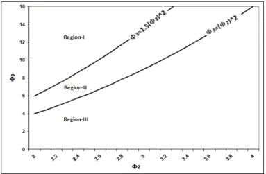
Note1: For the approximation to hold, it is necessary that s0≤0. Simple calculations show
that this condition implies that Ф2>2 and Ф3≥(3/2)Ф22 or Ф2<2 and Ф3≤(3/2)Ф22 (see Figure 1), where C2 is the squared coefficient of variation of inter-arrival time, Ф2= C2+1, and Ф3=m3/m13.
Figure1: Feasible regions for the approximation
Note2: It is worth mentioning that the error in the approximation (4) is of o(1) as s →0.
Note3: The condition that s0 is non-positive, which is necessary for the approximation to
hold, is satisfied by many standard arrival distributions: uniform, gamma, mixed exponential, lognormal, Coxian (K2), mixture of Erlangian, and Weibull. Also s0 is non-positive for truncated normal and inverse Gaussian probability density functions under certain conditions.
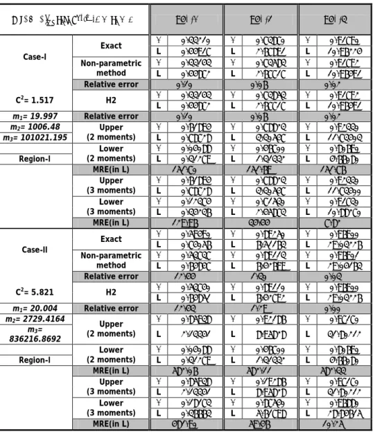
Using (4) in equations (2) and (1) with the values of m1, m2, and m3, the performance measures σ and L were obtained immediately. To illustrate the efficiency of the proposed method, we present (in Table 1) the values of σ and L computed using (4) for certain choices of the set {m1, m2, m3}. In order to compare the approximations with exact values, we have considered the values of the moments of commonly used arrival distributions – namely, gamma (Table 1) and PH4 distributions (Table 2). The values of σ and L are calculated for various values of traffic intensity ρ. Eckberg [5] specified upper and lower bound distributions that yield the maximum and minimum mean queue length in a steady state among all inter-arrival time distributions with two and three moments specified. Using these distributions, Whitt [16] calculated the maximum relative error for σ and L using the formula
where Ll and Lu are the minimum and maximum values of L using the lower and upper bound distributions. Table 1 also presents the upper and lower bounds for σ and L given two and three moments, and the corresponding maximum relative errors specified in (10). It can be seen that our method captures the values of σ and L with low relative errors.
Table1: Approximations for σ and L with gamma inter-arrival distribution
ρ=0.3 ρ=0.7 ρ=0.9 Case-I Exact σ 0.27991 Σ 0.68748 σ 0.89541 L 0.41661 L 2.23986 L 8.60503 Non-parametric method σ L 0.31799 0.43988 Σ L 0.71160 2.42714 σ L 0.90422 9.39653 Relative error 5.58% 8.36% 9.20% C2= 0.9091 Upper (2 moments) σ L 0.49760 0.59713 σ L 0.72080 2.50716 σ L 0.89890 8.90208 m1= 0.55 Lower (2 moments) σ 0.04880 σ 0.46700 σ 0.80690 m2= 0.5775 L 0.31279 L 1.31332 L 4.60798 m3= 0.8951 MRE(in L) 90.91% 90.90% 93.19% Upper (3 moments) σ 0.49760 σ 0.72080 σ 0.89890 Region-II L 0.59713 L 2.50716 L 8.90208 Lower (3 moments) σ 0.16180 σ 0.68076 σ 0.89520 L 0.35791 L 2.19271 L 8.58779 MRE(in L) 66.84% 14.34% 3.66% Case-II Exact σ 0.60233 σ 0.85242 σ 0.95297 L 0.75439 L 4.74319 L 19.13469 Non-parametric method σ L 0.55157 0.66900 σ L 0.85082 4.69232 σ L 19.11640 0.95292 C2= 3.3333 Relative error 11.31% 1.05% 0.03% m1= 0.45 Upper (2 moments) σ 0.77867 σ 0.87700 σ 0.95540 m2= 0.8775 L 1.35542 L 5.69106 L 20.17937 m3= 3.0273 Lower (2 moments) σ 0.04088 σ 0.46700 σ 0.80690 L 0.31279 L 1.31332 L 4.66080 Region-I MRE(in L) 333.34% 333.33% 332.96% Upper (3 moments) σ L 0.77867 1.35544 σ L 0.87700 5.69106 σ L 20.17937 0.95540 Lower (3 moments) σ 0.24600 σ 0.84200 σ 0.95270 L 0.39788 L 4.43038 L 19.02748 MRE(in L) 240.67% 28.46% 6.05%
3. INTER-ARRIVAL DISTRIBUTION APPROXIMATION BY MATCHING MOMENTS
Approximating general distributions by phase type distributions is important in queuing theory because their structure leads to Markovian state description and consequently analytical tractability. Although several phase type distributions have been used in the literature, two distributions that are prime candidates for such approximations (because of their simplicity and suitability) are mixtures of two exponentials (H2) and Coxian (K2) distributions. On this point, we use the former for analysis, as these distributions provide a fairly accurate match when the C2 is large – which is true for arrival distribution in a queuing system. Furthermore, in some of the examples discussed by Whitt [17], the maximum relative error (MRE) when two moments are fitted was found to be 200 percent, while working with mixtures of exponentials reduced the MRE to 50 percent. Specifying the third moment reduced the MRE to 5 percent. Thus, a three-moment match using H2 distributions for inter-arrival distributions seems to provide useful results.
Using an empirical study, Bere [3] showed that when the service time distribution is approximated using the first two of its moments, the third moment has a considerable effect on the probability distribution of the number of customers in an M/G/1 queue if
C2>1. He also showed that the probability distribution of the number of customers and the average number of customers in λ(n)/G/1/N system are highly sensitive to the third moment of the service time distribution if C2>1. Altiok [1], in justifying the inclusion of the third moment in matching, refers to Bere’s empirical work. Whitt [15] empirically showed that the effect of the third moment on the average number in the system in a GI/G/1 queue becomes considerable as C2 increases. If the service time distribution has C2<1, the impact of the third moment is not significant [3, 15]. Since the present work deals with matching an H2 distribution with three moments, we confine our attention to the range C2>1 only.
It is well known [15] that three numbers m1, m2, and m3 can be the first three raw moments of a distribution function F, provided that m1≥0, m2/m12≥1, and m3/m13≥ m22/m14. Furthermore, if the first three moments exist for a distribution F, then an H2 distribution exists with these three moments if, and only if, the first three moments of F satisfy the conditions m1≥0, Ф2=m2/m12 = C2 +1 ≥ 2, and Ф3 =m3/m13 ≥ (3/2) Ф22 [1]. However, Karlin & Studden [7] have shown that m1, m2, and m3 are the moments of some probability distributions on the positive real line if, and only if, m1≥ 0, Ф2≥ 1, and Ф3≥ Ф22. Thus, in the region where exact three-moment matching is not possible, researchers have used adhoc methods to find the approximate H2 distribution. These regions are clearly shown in Figure 2.
Figure 2: Region of three-moment matching (Region-I: Exact three-moment match possible; Region-II: Exact three-moment match not possible; Region-III: Infeasible region
for three moments of a distribution function)
The parameters p, μ1, and μ2 of H2 (see (11) below) when (m1, m2, m3) falls in Region-I, and where the three moments can be matched exactly, are well documented. However, when these moments fall in Region-II, such that the three moments cannot be matched exactly, methods suggested in the literature are recipes in nature. Lopez-Herrero [10], in the absence of information on service distribution, used the maximum entropy principle approach to estimate the true distribution of the number of customers served during the busy period in an M/G/1 retrial system. Whitt [15] suggests that “if m3 turns out to be too small when attempting an H2-fit, one procedure is to replace m3 by something slightly larger than (3/2) m22/m1”. Altiok [1] suggests the use of m3 = 3m22/2m1 + εm13 but does not indicate how to calculate the perturbation parameter ε. In the following algorithm, we propose a goal programming procedure of matching the first two moments exactly, and matching the third moment as closely as possible in Region-II. This procedure subsumes Region-I as a particular case. We note that Region-III is an infeasible region for the existence of (m1, m2, m3).
Algorithm
Given the first three moments of a distribution function F (say, m1, m2, and m3, which are assumed to be finite), the parameters p (0<p<1), μ1, and μ2 of the H2 distribution given by (11) – whose first three moments either match m1, m2, and m3 exactly, or match the first two moments exactly, and match the third moment as closely as possible in the sense of squared differences – are given by the following algorithm:
Step 1: Find optimal p using the Golden section method [12, 6] to solve the following one
dimension optimisation problem:
1 1 2 1 2 < < + − = p C C MinZ
(
)
2 2 3 2 2 3 1 3 ) 1 ( 1 2 2 1 1 2 3 1 6 − − − + − + − p p p C C m mStep 2: Using the value of p found in step 1, compute:
(
)
− − − = 1 2 1 1 2 1 1 C p p m µ and(
)
(
)
− − + = 1 1 2 1 2 1 2 C p p m µThe steps of the algorithm are justified using the following arguments. Consider the following probability density function of a mixture of two exponentials (H2 distribution):
, 0 , exp ) 1 ( exp ) ( 2 2 1 1 ≥ − − + − = x x p x p x f µ µ µ µ 0≤ p≤1 (11)
In the following, we do not consider the trivial cases of p=0, 1 as they lead us to exponential density.
The first three moments of the density function above are: 2 1 1 p
µ
(1 p)µ
m = + − (12) 2 2 2 1 2 2pµ
2(1 p)µ
m = + − (13)[
3]
2 3 1 36
p
µ
(
1
p
)
µ
m
=
+
−
(14) From (12) we have p p m − − = 1 1 1 2 µ µ (15)Substituting (15) in (13), and after simple algebra
(
)
− − ± = 1 2 1 1 2 1 1 C p p m µ (16)(
)
− − − = 1 2 1 1 2 1 1 C p p m µ (17) We know that(
1)
0 2 1− C2− ≥ pp , which implies that C2≥1 Also, μ1>0 implies that
1 1 2 2 + − > C C p (18) Substituting (17) in (15) results in
(
)
(
)
− − + = 1 1 2 1 2 1 2 C p p m µ (19)The third parameter p is obtained by matching the third moment as closely as possible. Thus, we minimise
(
)
2 2 3 2 2 3 1 3 ) 1 ( 1 2 2 1 1 2 3 1 6 − − − + − + − p p p C C m m (20) subject to: 1 1 1 2 2 + − > > C C pIn the second case, we set
(
)
− − + = 1 2 1 1 2 1 1 C p p m µ (21)Using algebra similar to the first case results in
(
)
(
)
− − − = 1 1 2 1 2 1 2 C p p m µ (22)and the third parameter p is determined by solving 0 1 2 2 > > + = p C MinZ
(
)
2 2 3 2 2 3 1 3 ) 1 ( 1 2 2 1 1 2 3 1 6 − − − + − + − p p p C C m m (23)It is easily seen that both cases lead to the same result, but with the roles of p and 1-p interchanged.
In Table 2 we continue with PH4 inter-arrival distribution. To illustrate this, we fit H2 distribution for this distribution by matching the moments specified by the algorithm. The performance measures σ and L obtained by using the fitted H2 distribution in steps 1 and 2 are given in Table 2. Attention is drawn to the MRE for these measures when three moments are matched [16] and to the actual relative error in using the approximated H2 distributions. Also note that these two methods improve in accuracy for increasing ρ as expected.
Table 2: Approximations for σ and L with PH4 inter-arrival distribution 𝑓(𝑡) = ∑ 𝑝4𝑖=1 𝑖𝜆𝑖 𝑒−𝜆𝑖𝑡 , 0 < 𝑝𝑖< 1 ρ=0.3 ρ=0.7 ρ=0.9 Case-I Exact σ L 0.33210 σ 0.73870 σ 0.91790 0.44917 L 2.67891 L 10.96224 Non-parametric method σ L 0.33143 0.44872 σ L 0.73583 2.67717 σ L 10.96491 0.91792 Relative error 0.10% 0.06% 0.02% C2= 1.517 H2 σ 0.33143 σ 0.73853 σ 0.91792 L 0.44872 L 2.67717 L 10.96491 m1= 19.997 Relative error 0.10% 0.06% 0.02% m2= 1006.48 Upper (2 moments) σ 0.61894 σ 0.78823 σ 0.92330 m3= 101021.195 L 0.78728 L 3.30547 L 11.73403 Lower (2 moments) σ 0.04088 σ 0.46700 σ 0.80690 Region-I L 0.31279 L 1.31332 L 4.66080 MRE(in L) 151.70% 151.69% 151.76% Upper (3 moments) σ 0.61894 σ 0.78823 σ 0.92330 L 0.78728 L 3.30547 L 11.73400 Lower (3 moments) σ 0.12374 σ 0.71530 σ 0.91730 L 0.34236 L 2.45873 L 10.88270 MRE(in L) 129.96% 34.44% 7.82% Case-II Exact σ 0.59490 σ 0.89250 σ 0.96900 L 0.74056 L 6.51163 L 29.03226 Non-parametric method σ L 0.53737 0.64847 σ L 0.89113 6.42699 σ L 29.04163 0.96901 Relative error 12.44% 1.30% 0.03% C2= 5.821 H2 σ 0.53740 σ 0.89110 σ 0.96900 L 0.64851 L 6.42792 L 29.03226 m1= 20.004 Relative error 12.43% 1.29% 0.00% m2= 2729.4164 Upper (2 moments) σ 0.85938 σ 0.92186 σ 0.97170 m3= 836216.8692 L 2.13341 L 8.95828 L 31.80212 Lower (2 moments) σ 0.04088 σ 0.46700 σ 0.80690 Region-I L 0.31279 L 1.31332 L 4.66080 MRE(in L) 582.06% 582.11% 582.33% Upper (3 moments) σ 0.85938 σ 0.19286 σ 0.97170 L 2.13341 L 8.95828 L 31.80212 Lower (3 moments) σ 0.18173 σ 0.87540 σ 0.96880 L 0.36663 L 5.61798 L 28.84615 MRE(in L) 481.90% 59.46% 10.25%
4. TWO OPTIMISATION ILLUSTRATIONS 4.1 Illustration 1
In practice, queuing managers are generally interested in optimising the model parameters under their control by minimising the operating cost or maximising the business profit. In the first illustration, we will be interested in obtaining the optimal service rate in a cost minimisation problem for a GI/M/1 queuing system. The objective cost function consists of two components: the cost due to customers waiting in line (known as the delay cost), and the service cost rate. Thus the cost function to be minimised is given by:
𝐶(𝜇) = 𝑐1(𝜆𝑊) + 𝑐2𝜇 (24)
where λ and µ are the arrival and service rates respectively, W is the expected waiting time of a customer in the system, c1 is the expected cost per unit time of a customer’s wait, and c2 is the service cost rate. Using Little’s formula, (24) reduces to
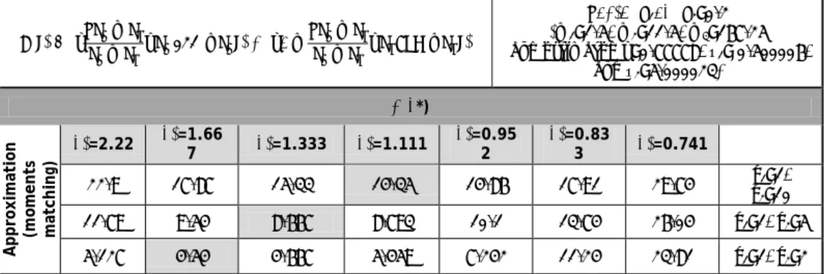
𝐶(𝜇) = 𝑐1𝐿 + 𝑐2𝜇 (25) The optimal µ* of the objective function above was computed using our moments matching method (introduced in section 3) by assuming the first three moments of the arrival distribution only, and the cost rates. However, in order to compare our results with the exact values, the moments were chosen to correspond to Coxian (K2) and Inverse Gaussian distributions commonly used in queuing theory. The results are presented in Tables 3 and 4. When the Coxian arrival distribution was used, our method provided the exact values of µ*. In the case of Inverse Gaussian distribution, the relative errors were significantly small.
Table 3. The optimal service rate µ* with Coxian inter-arrival distribution. (The optimal µ* computed, using our method and using the Coxian distribution, match exactly)
𝑓(𝑡) = �𝜌𝜆𝜆1− 𝜆2 1− 𝜆2� 𝜆1exp(−𝜆1𝑡) + �1 − 𝜌𝜆1− 𝜆2 𝜆1− 𝜆2� 𝜆2𝑒𝑥𝑝(−𝜆2𝑡) ρ=0.8, λ1=2, λ2=0.2 (m1=1.5, m2=11.5, m3=167.25 and estimated p=0.77778, µ1= 0.500006, and µ2=5.000023) C(μ*) A pp ro xi m at io n (m om ents m atc hi ng ) μ*=2.22 μ*=1.66 7 μ*=1.333 μ*=1.111 μ*=0.952 μ*=0.833 μ*=0.741 22.9 17.87 15.33 14.35 14.86 17.91 29.74 c1=1, c2=10 11.79 9.54 8.667 8.793 10.1 13.74 26.04 c1=1, c2=5 5.127 4.54 4.667 5.459 7.242 11.24 23.81 c1=1, c2=2 Table 4. The optimal service rate µ* with Inverse Gaussian inter-arrival distribution
K=1, M=2 (m1=2, m2=12, m3=152 and estimated p=0.8430, µ1= 1.3897, and µ2=5.27770) C(μ*) Ex ac t va lue s μ*=1.667 μ*=1.25 μ*=1.00 μ*=0.833 μ*=0.714 μ*=0.625 μ*=0.556 17.126 13.255 11.193 10.215 10.213 11.76 18.505 c1=1, c2=10 8.793 7.005 6.193 6.048 6.642 8.635 15.727 c1=1, c2=5 3.793 3.255 3.193 3.548 4.499 6.76 14.061 c1=1, c2=2 A pp ro xi m at io n (m om ents m at chi ng ) 17.139 13.265 11.198 10.213 10.206 11.750 18.505 cc21=10 =1, 8.806 7.015 6.198 6.046 6.635 8.625 15.727 cc12=1, =5 3.806 3.265 3.198 3.546 4.492 6.750 14.061 cc12=1, =2 Relative error = 0.14% 0.03% 0.07% 4.2 Illustration 2
In the second illustration, we consider an optimisation problem in a GI/M/1 queue with working vacation for the server. These problems have wide application in Internet systems such as optical, electrical, and communication nets [8]. We consider a single server queuing system that has the general arrival process. The working vacation and vacation interruption are connected, and the server enters into vacation when there are no customers, and it can take service at the lower rate during the vacation period. If there are customers in the system at the instant of a service completion during the vacation period, the server will
− − = t M M t K t K t f 2 2 2 1 3 2 ) ( exp 2 ) (
π
return to the normal working level regardless of whether the vacation ends. Otherwise, it continues the vacation. The performance measure L, the mean queue length, and P(J=0) and P(J=1) – which are the state probabilities of a server in the steady state - have been derived by Li et al. [8]. We refer the reader to their paper for the relevant expressions. Li et al. [8] considered the problem of optimising the service rate η during the server’s vacation period for a given cost structure. Let cw represent the unit time cost of every waiting customer, and c1 and c2 the service costs per unit time during the normal working level and vacation period respectively. The expected net cost function to be optimised can be seen to be
min: Z = cw L + c1 µ P(J=1) + c2 η P(J=0) (26)
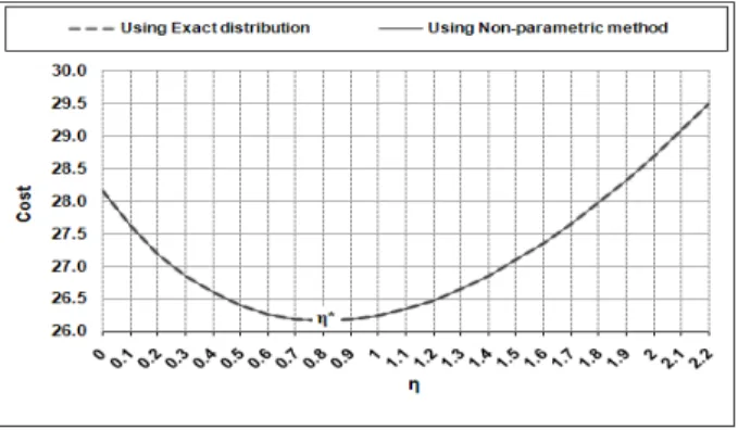
where µ is the service rate during the service period. The optimal service rate η* was computed using our non-parametric method of section 2 for certain values of the model parameters and cost parameters. We have used the Coxian arrival distribution and its moments (as used in Illustration 1) to obtain the optimal service rate η*. However, the Inverse Gaussian distribution could not be used, as the objective function (26) loses its convexity and becomes monotonic. We have used Erlangian of order 2 (used by Li et al. [8]) in its place. In Figures 3 and 4, we present the values of η versus the associated cost. The optimal η* and the corresponding cost obtained using our method are very close to the exact values.
Figure 3: (cw=4, c1=15, c2=10, Θ=1, ρ=0.65, and Coxian distribution parameters are
p=0.8, λ1=2, λ2=0.2) Optimal service rate η* during servers vacation period with Coxian
inter-arrival distribution
Figure 4: (cw=4, c1=15, c2=10, Θ=1, ρ=0.65, and Erlangian distribution parameters are
K=2, M=2.5) Optimal service rate η* during servers vacation period with Erlangian of
5. CONCLUSION
This study introduces two methods for evaluating performance measures in a GI/M/1 queuing system in the absence of information on the arrival distribution, and when only the first three moments are known. The first method is non-parametric as it does not use the distribution function, whereas the second method uses an H2 distribution obtained by moment matching procedure. This procedure involves the computationally economical Golden section method. Note that a Coxian (K2) distribution is also a good phase type distribution to consider. It is worth pursuing the regions (Ф2, Ф3) in which each of these approximations scores higher than the others in terms of relative errors. The usefulness of the methods in optimisation procedures has been illustrated with examples.
REFERENCES
[1] Altiok, T. 1985. On the phase-type approximations of general distributions. IIE Transactions,
17(2), pp 110-116.
[2] Baba, Y. 2005. Analysis of a GI/M/1 queue with multiple working vacations. Operations Research
Letters, 33(2), pp 201-209.
[3] Bere, B. 1981. Influence du moment d’ordre 3 sur les files d’attente a lois de services
generales. Thesis (MS). Universite de Rennes, France.
[4] Chae, K.C., Lim, D.E. & Yang, W.S. 2009. The GI/M/1 queue and the GI/Geo/1 queue both with
single working vacation. Performance Evaluation, 66(7), pp 356-367.
[5] Eckberg, A.E. 1977. Sharp bounds on Laplace-Stieltjes transforms, with applications to various
queuing problems. Mathematics of Operations Research, 2(2), pp 135-142.
[6] Kambo, N.S. 1991. Mathematical programming techniques, revised edition, East-West Press
Private Limited.
[7] Karlin, S. & Studden, W.J. 1966. Tchebycheff systems: With applications in analysis and
statistics. New York: John Wiley & Sons.
[8] Li, J., Tian, N. & Ma, Z. 2008. Performance analysis of GI/M/1 queue with working vacations and
vacation interruption. Applied Mathematical Modeling, 32(12), pp 2715-2730.
[9] Lindsay, B.G., Pilla, R.S. & Basak, P. 2000. Moment-based approximations of distributions using
mixtures: Theory and applications. Ann. Inst. Statist. Math, 52(2), pp 215-230.
[10] Lopez-Herrero, M.J. 2002. On the number of customers served in the M/G/1 retrial queue: First
moments and maximum entropy approach. Journal of Computers and Operations Research, 29(12), pp 1739-1757.
[11] Neuts, M.F. 1981. Matrix geometric solutions in stochastic models: An algorithmic approach.
John Hopkins University Press.
[12] Rao, S.S. 2009. Engineering optimization: Theory and practice. 4th edition, John Wiley & Sons. [13] Smith, J.M. 2011. Properties and performance modeling of finite buffer M/G/1/K networks.
Journal of Computers and Operations Research, 38(4), pp 740-754.
[14] Sohn, S.Y. & Lee, S.H. 2004. Sensitivity analysis for output performance measures in long-range
dependent queuing system. Journal of Computers and Operations Research, 31(9), pp 1527-1536. [15] Whitt, W. 1982. Approximate a point process by a renewal process, I: Two basic methods.
Operations Research, 30(1), pp 125-147.
[16] Whitt, W. 1984. On approximations for queues, I: Extremal distributions. AT&T Bell Laboratory
Technical Journal, 63(1), pp 115-138.
[17] Whitt, W. 1984. On approximations for queues, III: Mixtures of exponential distributions. AT&T
Bell Laboratory Technical Journal, 63(1), pp 163-175.
A A A A A A A A A A A A A A A