Evaluation of the Turkish army soldier recruitment system and a model proposal for the optimization of soldier recruitment system

(1)

EVALUATION OF THE TURKISH ARMY SOLDIER RECRUITMENT SYSTEM AND A MODEL PROPOSAL FOR THE OPTIMIZATION OF SOLDIER

RECRUITMENT SYSTEM

The Institute of Economics and Social Sciences

of

Bilkent University

by

AHMET YÜKSEL

In Partial Fulfilment of the Requirements for the Degree of Master of Business Administration

In

THE DEPARTMENT OF MANAGEMENT BILKENT UNIVERSITY

ANKARA

(2)

I certify that I have read this thesis and have found that it is fully adequate, in scope and in quality, as a thesis for the degree of Master of Business Administration.

--- Prof. Erdal EREL

Supervisor

---

Prof. Abdülkadir VAROĞLU Examining Committee Member

--- Asst.Prof. Levent AKDENİZ

Examining Committee Member

Approval of the Institute of Economics and Social Sciences

--- Prof. Erdal EREL Director

(3)

i

ABSTRACT

EVALUATION OF THE TURKISH ARMY SOLDIER RECRUITMENT SYSTEM AND A MODEL PROPOSAL FOR THE OPTIMIZATION OF SOLDIER

RECRUITMENT SYSTEM Yüksel, Ahmet

Master of Business Administration, Department of Management Supervisor: Prof. Erdal EREL

September 2005

This study evaluates the Turkish Army recruitment system by measuring the total deviations of personnel inventories from the target value of inventory level. The target inventory level is the average of projected available human source in the next 19 years. In our study we offer a model that minimizes the deviations from the targeted inventory level of soldiers. The study also computes the zero value of total number of deviations for different service time durations in the military with applying different ages for the people of same birth year at the time of recruitment. The results of the study indicate that even without the flexibility of applying different ages, the model always achieves better results than the current recruitment system.

(4)

ii ÖZET

TÜRK ORDUSU ASKERE ALMA SİSTEMİNİN DEĞERLENDİRİLMESİ VE ASKERE ALMA SİSTEMİNİN OPTİMİZASYONU İÇİN BİR MODEL ÖNERİSİ

Yüksel, Ahmet

Yüksek Lisans Tezi, İşletme Fakültesi Tez Yöneticisi: Prof. Erdal EREL

Eylül 2005

Bu çalışma Türk Ordusu askere alma sistemini değerlendirmektedir. Bu değerlendirme 19 yıllık bir dönemde her dönem askere alınacak insan miktarlarının 19 yıllık ortalamasından oluşan değerden yıllık toplam asker miktarlarının sapmasının hesaplanması ile yapılmaktadır. Ayrıca hedef değerden oluşan bu sapmaları minimize edecek bir model önerilmektedir. Bu çalışma ayrıca askerlik hizmet süresinin değiştirilmesi ve askere alınma yaşlarının aynı yıl doğmuş insanlar için farklı uygulanması ile sağlanan esneklik sonucunda sıfır sapma sağlayabilecek hedef asker miktarı değerlerini de bulmaktadır. Çalışmanın sonuçları göstermektedir ki farklı askerlik yaşı uygulamasının esnekliği olmadan bile model her zaman uygulanmakta olan sistemden daha iyi sonuçlar vermektedir.

(5)

iii

ACKNOWLEDGEMENTS

I would like to thank to Prof. Erdal EREL for his guidance and patience during the preparation of this thesis. I would like to thank to Prof.Abdülkadir VAROĞLU and Asst.Prof.Levent AKDENİZ for their kind contributions and advices. I would like to express my special thanks to my friend Sezen for his technical support. Finally I am grateful to my wife Ayşe for her dedicated support throughout my study.

(6)

iv TABLE OF CONTENTS ABSTRACT……… ...

i

ÖZET……….. ...

ii

ACKNOWLEDGEMENTS………... ...

iii

TABLE OFCONTENTS……….. ... .

iv

LIST OF TABLES………..……….. ...

vi

1. CHAPTER 1: INTRODUCTION………... 1

1.1. The Current Recruitment System In The Turkish Army………….... 1

1.2. Motivation For The Thesis……… ... 1

1.3. The Use of Army Manpower Planning Systems……… .... 2

1.4. Recruitment Of Soldiers In The Turkish Army……… ... 3

1.5. Method ... 5

2. CHAPTER 2: LITERATURE REVIEW ... 7

2.1. The Army Manpower Long-range Planning System ... 8

2.2. Greedy Heuristics Algorithms For Manpower Shift Planning ... 10

2.3. Modeling The Officer Recruitment and Manpower Planning Process In the Turkish Land Forces ... 15

2.4. Comparison of The Thesis... 36

(7)

v

3.1. The Definition Of The Problem ... 37

3.2. Assumptions……... 37

3.3. The Formulation Of The Problem ... 38

4. CHAPTER 4: EXPERIMENTATION... 52

5. CHAPTER 5: SUMMARY AND CONCLUDING REMARKS ... 58

(8)

vi

LIST OF TABLES

1. Table 1 The List of Corresponding Calendar Years for the Periods of Recruitment ... 40 2. Table 2 The Deviation Numbers and The Ratios of

Deviations To The Target Value ... 55 3. Table 3 Total Inventory Levels Corresponding to Each

Periods For The Current Recruitment System ... 56 4. Table 4 Total Inventory Levels Corresponding to Each

(9)

1

CHAPTER 1

INTRODUCTION

1.1.The Current Recruitment System In The Turkish Army

The recruitment system in our country, which is being implemented, is founded on the system of military service by obligation. This system did not change much in time having small modifications and additions that tried to compensate for the needs of the time. The current system is based on recruiting people at the age of 20 and after a basic training period, employing them for 12 months. Since the recruitment is done every three months, the employment is also done every three months.

1.2. Motivation For The Thesis

I decided for the subject of my thesis after working on the population growth data for Turkey. The data indicates that the childbirths have sharply declined in the recent years. I decided to construct a model that compensates for the

(10)

2

fluctuations of the birthrates which will affect the human source of the Army. The model first has to compute the optimum levels of the numbers of recruited soldiers and second it has to decrease the fluctuations of the total numbers of soldiers that change from year to year because of the changes in the human source. The model must be constructed in such a way that the resulting total soldier numbers must satisfy the need in terms of numbers of soldiers for each time period.

1.3. The Use of Army Manpower Planning Systems

The manpower planning systems are used in the armies (2) to solve the following problems:

1- Evaluate the effects of current policies in a long time period generally up to 20 years.

2- Compare the inventories resulting from the current policies to the desired needs of the army.

3- Determine the types of policies needed to reach the future end-strength targets by testing the projected results of applying these policies.

4- Evaluate the army’s ability to reach the target inventory levels by using these new policies.

(11)

3

The manpower planning models help the manpower planners to determine the optimal transition rates, promotion rates, and observe the effects of attrition rates based on the historical statistical data.

1.4. Recruitment Of Soldiers In The Turkish Army

Soldier recruitment is a very wide field in terms of the variety of the recruitment methods. The most frequently used methods were recruitment of people by obligation for the military service, recruitment by random selection, voluntary recruitment and recruitment of mercenaries. These were the main recruitment methods but mostly a mixture of these methods was applied in the world armies.

The most practical and the best model for the whole European countries was the Prussian Army System (4). Prussians, in addition to their disciplined soldiers, were adept in constructing a robust system of recruitment and training of the soldiers. The system was very simple and applicable. They recruited small portions of people in the peacetime, trained them for short time periods and let them back after the training. They also had a small core of professionals on hand. Thus, they carried the burden of a small army while they can always recruit a huge number of trained people ready to be employed in the hinterland.

(12)

4

In our history army was the primary priority for all the Turkish states(5). In the old days it was a voluntary duty for people to be in the military. The nature of the way of living in the Turkish nation was somehow in conformity with the military service. That is the reason why Turks were employed as soldiers in the non-Turkish countries they lived.

Turkish countries founded in controversial regions of the world, developed different ways of recruiting armies. At the first stages of the Ottoman Empire when it was a small state, the recruitment was somewhat a very simple system of calling people at war times for the defense of the country. At the time of Murat I. a professional army was founded called ‘Yeniçeri Ocağı’ which resulted from the heavy clashes with the Eastern Roman Empire and the Balkan nations. This army’s human source was the non-Muslim people that were trained from the childhood in order to execute the duty of a soldier as professionals.

In 1847 a new act was accepted (4) organizing the criteria of recruitment in fields as the penalties for the acts of abstaining from the obligation for military service, the conditions for exemption from the obligation, payment of compensation for military service and the maximum age to be recruited at.

For the problems of the system in 1869, a new order was accepted calling for the army to have three types of soldiers which were ‘Nizamiye’, ‘Redif ‘ and ‘Müstahfaz’ that Nizamiye soldiers were the known type of soldiers recruited when they reached the age of recruitment and done the duty for a

(13)

5

certain period then were discharged. The Redif and Müstahfaz soldiers were reserves that expected to be called for war and crisis times of the country for a predetermined time period. The soldiers after the Nizamiye duty were sent home as Redif soldiers. Redif period was for six years and there was a one-month training for the Redif Soldiers that was done in every six years.

The people who chose to pay a compensation to comply with the military obligation were also recruited for a training period of 5 months. Also the people who chose to pass their Redif period as Nizamiye and the people who chose to serve an extra time for a salary were employed for six years.

The system of soldier recruitment changed to the current military obligation system in 1927 making everyone responsible for the military service.

1.5. Method

The age constraint which is 20 years for people who will be recruited had to be loosened in order to make it possible to recruit a group of people having the same birth year in different ages in other words employ them not in a fixed year as it is done in the current system but in different years when needed. I built the system mathematically using linear goal programming in the light of the parameters, which are the male childbirth numbers in years that will make the human source of the Army in the projected future and the attrition rates. The variables of my problem were the optimal accessions at

(14)

6

the beginning of each time period, the inventory numbers for every accession after attritions caused by reasons such as death and diseases or accidents that make it impossible for the people to continue with the military service.

The ages of the soldiers at the accession time can differ according to their education levels which are classified as sources in our model as 18-23 ages for the people having education level of up to basic education of 8 years, 20-24 for high school graduates and 23-27 for university graduates. Also the Army can call anyone out of his will anytime in order to fulfill the personnel inventory.

(15)

7

CHAPTER 2

LITERATURE REVIEW

Using optimization or simulation are very widely used and robust methods for the personnel planning purposes. There are a great number of studies done about the long-range personnel planning; some of them are for academic purposes and the others are for the practical use of corporations or government organizations.

These studies are constructed generally using Markov chains. The method offers for the optimal number of personnel accessions at the beginning of each chosen time period by combining the scheduling process with the amortization of the personnel inventory happening during the period. The personnel planning model has to satisfy the constraints of the organization such as the minimum number of the personnel inventory to be achieved at each time period, the job experience in terms of time passed in certain positions. Another constraint is that the total of accessions in a certain time period must not exceed maximum number of people that is thought to be available at the time of recruitment, i.e. the amount of the source. The

(16)

8

amortization of the personnel inventory is done because of the attrition of people for such reasons as death, disease and departure from the organization. Another reason for the amortization of the inventory is transition, which includes the reasons as promotion or change of position in the organization itself. The model must have an objective function, which will find the optimal number of personnel accessions for the objective function defined in the model.

There are a number of studies done in the literature about personnel planning. Three of these studies will be presented. The first one is a study that explains the recruitment system of the U.S. Army. The second one is a different type of formulation of the personnel planning in the food industry and the third one is an application of the military personnel planning in the Turkish Army Land Forces for officer recruitment.

2.1. The Army Manpower Long-range Planning System

The system of Army Manpower Long-range Planning (2) enables the army officials to develop long-range plans by providing them with the robust analytical capability to project the strength of the American Army for 20 years. The model simulates the effects of gains, losses, promotions and reclassifications in terms of personnel to help the planners or analysts to determine the changes in the recruitment systems or in the personnel education policies to reach a desired force. The mathematical model helps

(17)

9

the planners see the future personnel numbers by forecasting the probable effects of the gains, losses, personnel policy changes or transition of the personnel’s skills by education.

The need for managing a multi-attribute pool of personnel over a long-term planning horizon resulted in the development of a series of linear programming and Markov chain- based approaches for assessing the policy options. A series of studies were done as army personnel models to determine the number of personnel -soldiers or officers- based on the factors of grade, skill and years of service subject to the constraints of new personnel accessions from out of the organization, separations from the organization and promotion policies in order to meet the manpower goals of the army in a planning time period of 7 to 20 years.

A typical personnel goal-programming model is structured in the following manner.

Grade-Skill Target Constraints:

INVX(t, g, s) + TARP(t, g, s) – TARN(t, g, s) = TARG(t,g,s).

For each grade g and skill type s in year t, when the total inventory INVX(t,g,s) is not equal to the targeted strength goal which is TARG(t,g,s) for that skill and grade in that year, then a shortage is noted by TARP(t, g, s) and a surplus is noted as TARN(t,g,s).

(18)

10 Promotion Goal Constraints:

PROX (t, g, s )+PROP(t, g, s )-PRON(t, g, s ) = RPRO(t-1, g-1, s)* INVX(t-1, g-1, s).

The desired number of promotions to grade g during year t is the rate of promotion RPRO(t-1, g-1, s) times the year t beginning inventory INVX(t-1, g-1, s) in grade g-1 for all skills s. if the number of promotions PROX (t, g, s ) is less than the desired number of promotions or promotion goal in other words, then a shortage is added to PROX (t, g, s ) as PROP(t, g, s ) or a surplus is subtracted from it as PRON(t, g, s ).

The total of the deviation variables which are TARP(t, g, s), TARN(t, g, s), PROP(t, g, s ) and PRON(t, g, s ) are minimized by assigning them in the objective function multiplied by relative weights given for each of them.

2.2. Greedy Heuristics Algorithms For Manpower Shift Planning

Greedy Heuristics Algorithms For Manpower Shift Planning (3) is a study done for the solution of personnel planning problem in a food packaging company. In companies like the foods industry or pharmaceuticals, the operations like packaging are very simple. These operations are done in lines consisting of dedicated and specialized machines with usually one skilled operator and several unskilled workers. These unskilled workers are

(19)

11

hired to work on a certain workday shift for generally one month with a one-month contract. At the end of the contract the workers are fired to be recalled later and they are recruited again if needed. Workers cannot be fired before the end of their contracts’ expiration.

In production plants as explained, the total work requirements are structured for one-month period master production schedules. These master production schedules give the total production load of each line for all products it manufactures. The production capacity of each packing line directly depends on the number of unskilled workers being employed in the line. The main planning problem for the management is to decide how many workers to employ in every daily workshift of a certain month in order to satisfy the production load of the each line. This will result in the maximization of the workforce utilization. The objective function however is set to minimize the total workforce to be employed in the production line. This kind of manpower planning is referred to as manpower shift planning problem.

Problem Formulation

A machine shop consists of n independent machines and work p shifts per day. Each machine i requires

a

_i unskilled workers and has a production load of

w

_i shifts (time periods). The MSP problem calls for the determination of the minimum number of workers to be employed in each

(20)

12

shift in order to complete the production load of each machine within a predetermined time horizon of d days.

Assumptions:

1- The workforce is flexible and can work on any machine.

2- The workforce is employed for a particular shift and cannot be employed in another shift.

3- The production load of each machine i covers an integer number of shifts and can be completed within the available time horizon (PD>

w

_i ).

4- There are no precedence relations between the machines i.e. they are independent of each other.

Mathematical Model:

Based on the definition explained above, the MSP problem is now formulated as an integer linear programming model. In this Integer Linear Programming (ILP) model we take the number of daily shifts as 3 (p= 3).

i

y

is the number of workers to be employed in shift i and

x

ij is an indicator variable taking the binary values of ‘1’ or ‘0’.

(21)

13

1 if machine j operates in period t.

ij

x

0 otherwise.

The period index t indicates a certain day and shift combination as follows : 0 < t < D for the day shift,

D < t < 2D for the evening shift, 2D < t < 3D for night day shift,

The workforce needed for the operation of machine j will be

a

j

x

ij.

Because the total workforce employed in at any period cannot exceed the available number of workers for the respective shift,

i tj n j j

y

x

a

≤

∑

=1 for all t and i.

Clearly, in order to complete its targeted production load, each machine j needs to operate for exactly

w

_j periods (possibly spread over all three shifts.). So: j D t tj

w

x =

∑

= 3 1 for all j. In brief: Minimize Z=Y1+Y2+Y3

(22)

14 ST . 0 1 1 ≥ −

∑

= tj n j j x a y 0<t ≤ D. . 0 2 1 ≥ −

∑

= tj n j j x a y D<t≤2D. . 0 3 1 ≥ −

∑

= tj n j j x a y 2D<t≤3D. . 3 1 j D i tj w x =

∑

= 1≤ j ≤n.

This study is a unique one made for the planning of the production in simple production lines which are directly affected by the number of workers. This type of personnel planning can be done by the help of personnel planning models regulates the number of the workers employed at the beginning of each period.

(23)

15

2.3. Modeling The Officer Recruitment and Manpower Planning Process In the Turkish Land Forces

This study is an example of personnel planning done for the officer recruitment and constructs a model that determines the optimal rank durations of the officers.

Because of the problem’s size and GAMS capacity (1), the problem is solved in two phases; phase1 and phase2. Phase1 is built for combat arms and phase2 is built for non-combat arms.

Both of combat and non-combat arms have no interaction among themselves. The only interaction is from combat arms to non-combat arms as a transition caused by health reasons making it impossible to continue with the combat missions. The transition out variables from combat arms to non-combat arms at the end of phase1 are taken to phase2 and inserted in the non-combat arms as transition in variables.

The officers in branches are acquired from six sources. The capacities of their sources have upper and lower bounds that are marked for each branch separate from each other.

(24)

16 Phase 1:

This phase is for the solution for the problem for the combat arms. Transitions in the problem can be summarized as one-way flow from combat to non-combat arms.

Phase 2:

This phase is for solving the manpower problem about the non-combat arms.

Indices:

T Set of calendar years. S Set of category cohorts. R Set of ranks.

I Set of branches. J Set of sources.

K Set of years of service. N Set of non-combat arms.

Calendar years t= 2001,2002, …,2029

Category Cohorts s= 1,2, …,28

(25)

17 Ranks

r= Second Lieutenant, First Lieutenant, Captain, Major, Lieutenant Colonel, Colonel

Branches(Combat)

i= Infantry, Armor, Artillery, Air Defense, Army Aviation, Signals, Engineers (only used in phase1).

Branches(Non-Combat)

i= Ordnance, Transportation, Personnel, Quartermasters, Finance (Used only in phase2).

Sources

j= Military academy, NCO’s (Type 1), NCO’s (Type2), CRO’s, Civilian, CO’s.

Years of service k= 1, 2, …,31

Non-Combat Arms

(26)

18

In the model in spite of the exception in station ceiling of the rank Colonel being 31 years, the maximum duration of service as an officer with no early promotions is 28 years. The officers from sources military academy, CRO’s, Civilian, enter the model with years of service ‘1’ and reach the last category cohort at the end of 28 years. The officers from source CO’s enter the model with years of service ‘1’ but promote to the rank of Captain at most and stay there until the station ceiling of this rank is completed which is 21 years. The officers from NCO’s (Type1) enter the model with years of service between 7 and 12 and move up to the rank of Colonel. The officers who will stay in the system maximum from this source are the ones who enter the system with 7 years of service. They reach the station ceiling of 31 years in the rank of Colonel. The officers from source NCO (Type2) enter the model at years of service between 7 and 9 and promote to the rank of Captain and stay there until the station ceiling of this rank that is 21 years. They can stay in the system for 14 years at maximum.

The ranks are divided into 28 category cohorts to match for the respective service year in the rank.

Initial Data and Parameters:

Mv(i, s, j, k) Given initial inventory for branch i, category cohort s, source j, with years of service k, in 2001.

(27)

19

Capl(i, j) Lower capacity of source j for branch i.

D(i, r) Strength goal of branch i, in rank r.

Tranti(t, i, s, j, k) Total transitions into branch i (non-combat arms), during year t, in category cohort s, for source j, with years of service k.

Ratt(i, s) Attrition rate for branch i and category cohort s.

Rpro(s) Normal promotion rate for category cohort s.

Rbpro(s) Early promotion rate for category cohort s.

Rtrano(i, s, n) Rate of transition out for branch i (combat arms), to branch n (non-combat arms), for category cohort s.

Wn(i, r) Weight given to negative deviations(shortfall) for branch i and rank r.

Wp(i, r) Weight given to positive deviations (surplus) for branch i and rank r.

Bf(i) Scalars to balance accessions from source Military Academy to branch i.

(28)

20 Variables:

Inv (t, i, s, j, k) Inventory at the beginning of year t, for branch i, category cohort s, from source j, with years of service k.

Invas (t, i, s, j, k) Inventory after attritions and transitions at the end of year t, for branch i, category cohort s, from source j, with years of service k.

Invtot (t, i, s) Total inventory at the beginning of year t, for branch i, category cohort s.

Rinv (t, i, r) Inventory at the beginning of year t, for branch i, rank r.

Acc(t, i, j, k) Officer accessions to the army at the end of year t, from source j, for branch i, with years of service k.

Tacc (t, i, j) Total officer accessions at the end of year t, from source j, for branch i.

Attr (t, i, s, j, k) Attritions during year t, for branch i, category cohort s, from source j, with years of service k.

Prot (t, i, s, j, k) Promotions to category cohort s at the beginning of year t, for branch i, category cohort s, from source j, with years of service k.

(29)

21

Notprof (t, i, s, j, k) Non-Promotions from category cohort s at the beginning of year t, for branch i, from source j, with years of service k.

Trano (t, i, s, j, k) Transitions from branch i to branch n during year t, in category cohort s, for source j, with years of service k.

Trano (t, i, s, j, k, n) Transitions from branch i to branch n during year t, in category cohort s, for source j, with years of service k.

Tranto (t, i, s, j, k) Total transitions from branch I, during year t, in category cohort s, for source j, with years of service k.

Gn (t, i, r) The amount under the authorized strength goal in year t, for branch i, rank r.

Gp (t, i, r) The amount over the authorized strength goal in year t, for branch i, rank r.

Constraints

Attrition Constraints: For all t,i,s,k, j=1,2,3,4,5

(30)

22

The attrition during year t and for sources, military academy (j=1), NCO(Type1) (j=2), NCO(Type2) (j=3), CRO’s(j=4), Civilian(j=5), is equal to the rate of attrition times the inventory at the beginning of year t.

For all t,i,s, j=6

Inv (t, i, s, j, k)* Ratt(i, s) , if k=3,6, …,30 Attr (t, i, s, j, k) =

0 , otherwise

The officers accessed to the army by contract can leave the army only at the end of the contract and the contracts are for 3 years. Hence the attrition during year t, for source COs (j=6), equal to the rate of attrition times the inventory at the beginning of year t, only for years of service k which are multiples of three.

Transition Constraints: For all t,i,s,j,k,n

Trano (t, i, s, j, k, n) = Inv (t, i, s, j, k)* Rtrano(i, s, n)

Transition out from branch i (combat arm) to branch n (non-combat arm), during year t is equal to the inventory at the beginning of year t times rate of transitions out from branch I to branch n.

(31)

23 Tranto (t, i, s, j, k) =

∑

n

Trano (t, i, s, j, k, n)

Total transition-out from branch i (combat arm) is equal to sum of the transitions out over n, from branch I (combat arm).

Inventory Constraints After Attritions and Transitions: (For Phase 1)

For all t,i,s,j,k

Invas(t, i, s, j, k) = Inv (t, i, s, j, k) - Attr (t, i, s, j, k) - Tranto (t, i, s, j, k)

The inventory at the end of year t is equal to the inventory at the beginning of year t minus the attritions during year t minus total transitions out from branch I (combat arm) during year t.

For Phase 2) For all t,i,s,j,k

Invas(t, i, s, j, k) = Inv (t, i, s, j, k) - Attr (t, i, s, j, k) - Tranti (t, i, s, j, k)

The inventory at the end of year t is equal to the inventory at the beginning of year t, minus the attritions during year t plus total transitions into branch i(non-combat arm) during year t. In phase 2, total transitions into branch I (non-combat arm) is parameter that is found from the arrangement of transition out variables in phase 1, according to non-combat arms.

(32)

24 Promotion Constraints:

NCO (Type 2) and contract officers cannot promote beyond the rank of a captain (category cohort 15). In some ranks there may be early promotions which are 8. and 14. category cohorts.

For all t,i,s and j=1,2,3,4,5

Prot (t+1,i,s,j,k+1) = Invas (t,i,s-1,j,k)*rpro(s-1)+Invas (t,i,s-2,j,k) * rbpro(s-2)

The promotions to category cohort s, at the beginning of year t+1, for sources, Military academy (j=1), NCOs (Type 1) (j=2), CROs (j=4), Civilian (j=5), with years of service k+1 is equal to the number of promoted officers from one category cohort below plus the number of early-promoted officers from two category cohorts below.

For all t,i, 1 < s ≤ 15 and j=3,6

Prot (t+1,i,s,j,k+1) = Invas (t,i,s-1,j,k)

The promotions to category cohort s greater than 1 and less than or equal to 15, at the beginning of year t+1, for sources NCOs (Type2) (j=3) and COs (j=6), with years t, in one category cohort below. Because the officers in one category cohort below promote to the next category cohort, since the promotion rate in one.

(33)

25 Prot (t+1,i,s,j,k+1) = 0

Remember than the officers from sources, NCOs (Type 2) (j=3), COs (j=6) can not promote beyond the rank of a captain (category cohort 15). Hence the promotion to higher category cohorts than 15, for sources NCOs (Type 2) and COs is zero.

For all t,i,s,j k=1 Prot (t+1,i,s,j,k) = 0

The promotions to any category cohort with year of service 1 is zero. Because an officer with year of service 1 is just in category cohort 1 and no promotion is available to category cohort 1.

Non-Promotion Constraints:

The non-promotion constraints are also branched because of different source characteristics.

For all t,i,j,k s=15

Invas(t,i,s,j,k) , if j=3, Notprot (t+1,i,s,j,k+1) = 0 , if j=1,2,4,5

(34)

26

The non-promotion from category cohort 15, at the beginning of year t+1 with years of service k+1 is equal to the inventory after attritions and transitions, at the end of year t, since the officers from sources NCOs (Type 2) (j=3), COs (j=6) can not promote beyond the rank of captain (category cohort 15).

For all t,i,j,k, s ≠ 15 Notprof (t+1,i,s,j,k) = 0

The non-promotions from other category cohorts should all be zero, since the total promotion rate (early promotion rate + normal promotion rate), from other category cohorts is 1.

For all t,i,s,j k=1

Notprof (t+1,i,s,j,k) = 0

(35)

27 Accession Constraints :

For all t, i, j=1 and k≠1, Acc(t,i,j,k)=0

The accessions to the army for sources j=1,4,5 and 6 with k≠1 are equal to ‘0’.

For all t,i, j=2 and k ≠ 7,8,9,10,11,12 Acc (t,i,j,k) = 0

The accession to the army, at the end of year t, from source NCOs (Type 1) (j=3), is only valid with years of service 7,8,9,10,11,12. Hence for other values of k, it is zero.

For all t,i, j=3 and k ≠ 7,8,9 Acc (t,i,j,k) = 0

The accession to the army, at the end of year t, from source NCOs (Type 1) (j=3), is only valid with years of service 7,8,9. Hence for other values of k, it is zero.

For all t,i,j Tacc (t,i,j) =

∑

k

(36)

28

The total accession to army from source j to branch i, at the end of year t is the sum of accessions over all k.

The accession and total accession variables are integer, hence we express the constraints in such a way that the constraints assign these variables to closest integer values.

For all t,i, j=2 and k=7,12 Acc(t,i,j,k) ≥ 0.1*Tacc(t,i,j)-1 Acc(t,i,j,k) ≤ 0.1*Tacc(t,i,j)+1

The accession to the army, from source NCOs (Type 1) (j=2), with years of service 7,12 is equal to %10 of total accession from the same source.

For all t,i, j=2 and k=8,9,10,11 Acc(t,i,j,k) ≥ 0.2*Tacc(t,i,j)-1 Acc(t,i,j,k) ≤ 0.2*Tacc(t,i,j)+1

The accession to the army, from source NCOs (Type 1) (j=2), with years of service 8,9,10,11 is equal to %20 of total accession from the same source.

(37)

29 Acc(t,i,j,k) ≥ 0.4*Tacc(t,i,j)-1

Acc(t,i,j,k) ≤ 0.4*Tacc(t,i,j)+1

The accession to the army, from source NCOs (Type 2) (j=3), with years of service 7 is equal to %40 of total accession from the same source.

For all t,i, j=3 and k=8,9 Acc(t,i,j,k) ≥ 0.3*Tacc(t,i,j)-1 Acc(t,i,j,k) ≤ 0.3*Tacc(t,i,j)+1

The accession to the army, from source NCO (Type 2) (j=3), with years of service 8,9 is equal to %30 of total accession from the same source.

Capacity Constraints :

For all t, j, k

Σ

Acc(t,i,j,k) < capu (i,j)

the total of accessions from source j, at the end of year t, to branch i is less than or equal to the upper capacity of source j for branch i.

For all t,i, j

(38)

30

The total of accessions from source j, at the end of year t, to branch i is greater than or equal to the lower capacity of source j for branch i.

Inventory Constraints :

An officer from any source starts to work in the army in the first category cohort. That means the accession to the army is only possible by the accession to the first category cohort.

The accession process according to sources and years of service that summarized the following three constraints can be seen in the Figure 3.3.

For all t,i,k, s=1 and j=1,4,5,6

Acc (t, i, j, k) , if k=1 Inv (t+1, i, s, j, k) =

0 , otherwise

The accession from sources, Military academy (j=1), CROs (j=4), Civilian (j=5) and COs (j=6) is only possible with years of service 1. The inventory in category cohort 1, at the beginning of year t+1, is equalto the accessions at the end of year t, with years of service 1. Since no accession is possible

(39)

31

from these sources, with other years of service values, the inventory in category cohort 1, with other years of service values is zero.

For all t,i,k, s=1 and j=2

Acc (t, i, j, k) , ifk=7,8,9,10,11,12 Inv (t+1, i, s, j, k) =

0 , otherwise

The accession from source NCOs (Type 1) (j=2) is only possible with years of service 7,8,9,10,11,12. The inventory in category cohort 1, at the beginning of year t+1, with years of service k is equal to the accessions at the end of year t, with years of service 7,8,9,10,11,12. Since no accession is possible from this source, for other years of service values, the inventory in category cohort 1 for other years of service values, is zero.

For all t,i,k, s=1 and j=3

Acc (t, i, j, k) , if k=7,8,9 Inv (t+1, i, s, j, k) =

0 , otherwise

(40)

32 For all t,i,j,s>1 and k=1

Inv (t+1, i, s, j, k)=0

For any category cohort greater than 1, there cannot be any accessions so the inventory for them is zero.

For all t,i,j,k, 1<s<3 ;

Prot (t, i,s, j, k) +Notprof(t,i,s, j, k) , if k<19 Inv (t, i, s, j, k) =

0 , otherwise

The inventory at the beginning of year t, in category cohort s greater than 1 and less than or equal to 3 (equivalent to rank Second Lieutinant), is equal to the promotions to category cohort s, plus the non-promotions from category cohort s.

Prot (t, i,s, j, k) +notprof(t,i,s, j, k) , if k<21 Inv (t, i, s, j, k) = 0 , if k>21

(41)

33 For all t,i,j,k, 15<s<20;

For all t,i,j,k, 20<s<23;

For all t,i,j,k, 23<s<28;

For all t,i,j,k, s>15 and j=3,6; Inv (t+1, i, s, j, k) = e =0

Inventory constraints for promotions and non-promotions.

For all t,i,s

Invtot(t,i,s) =

∑

k j

Inv (t, i, s, j, k)

(42)

34 Inv (t+1, i, s, j, k) = e =0

Total inventory at the beginning of year is equal to the sum of individual inventories.

Rank Constraints : For all t,i; r=1,

Rinv(t,i,r)=

∑

3 1 Intot (t, i, s) . . .

For all t,i; r=6, Rinv(t,i,r)=

∑

28

24

Intot (t, i, s)

The total inventories of each rank in year t for branch i is equal to the total sum of inventory over s over category cohorts of each rank.

(43)

35 Balance Constraints :

In order for the acccessions not to have great variations for the source military academy, the balance constraints were applied.

For all t,i,j=1,

Tacc(t+1,i,j) < Tacc(t,i,j) + Bf(i) Tacc(t+1,i,j) < Tacc(t,i,j) - Bf(i)

Deviation Constraints : For all t,i,r

D(i,r) = Rinv (t,i,r) + Gn(t,i,r) - Gp(t,i,r)

The authorized strength goal is equal to the rank inventory in year t, plus the amount under the authorized strength goal in year t minus the total amount over the authorized strength goal in year t.

Objective Function : Z=

∑

i t r

wn(i,r)*Gn(t,i,r) +

_∑

i t r

wp(i,r)*Gp(t,i,r)

The objective function is to minimize the weighted sums of the values of all the negative and positive deviations.

(44)

36

2.4. Comparison of The Studies In The Literature and My Thesis

My thesis is based generally on the idea held in the study mentioned in section 2.1. ‘The Army Manpower Long-range Planning System’. This study gives a general understanding of the system applied in the U.S. Army. The second study mentioned in section 2.2 was a civilian application of the manpower planning system. The study in section 2.3 was about officer recruitment planning system in the Turkish Army Landforces. This study is one of the first studies done for the personnel planning of the Turkish Army using linear programming. Thus, this study is the most relevant one to our study in the sense that it uses similar formulation for the solution of the problem.

My study differs from this one in the following: First, this study is held for the optimization of the Land Forces officer recruitment system while our study is for the optimization of the soldiers who are obliged for the military service and do the service doing the service as private corporal or sergeant. Second, the parameters in this study as promotion rates, transition rates and the rank constraints are not needed in our study. Last, the human source for the officer recruitment can be estimated while knowledge about the human source for the soldier recruitment can be roughly known with the historical data for birth numbers in years.

(45)

37

CHAPTER 3

MODEL

3.1.The Definition Of The Problem

The aim of our model is to decide for the number of soldiers that must be recruited in each period who will serve the military at a time horizon of 19 years to the future. These numbers must be determined such that the minimum possible numbers to serve in the army will be found in a way that the total number of personnel inventories at the end of time periods will satisfy the need for the number of soldiers for that period and the number of people between periods will not fluctuate in extreme numbers or there will be no fluctuations. The basic training period is out of the range of this study.

The aim of the study is to find the optimum recruitment periods with duration times of service that minimize the deviation of the total inventory numbers.

3.2. Assumptions

(46)

38

2. There will be no wars to cancel the execution of the system.

3. The ratios of each education levels will be same for the years in the scope of the study.

4. The attrition levels will not change in the following years.

5. The male population from the birth years held in the model is assumed to have done their military service before the new system is applied. 6. The male population under the consideration of the study will do their

service only in the projected future held in the 19 years time in the model but not then.

3.3. The Formulation Of The Problem

Indices:

t: Set of calendar years.

i : Set of calendar years for the year of birth.

k: Set of periods of a year for the recruitment of the people.

s: Set of sources.

(47)

39

Set of calendar years: t= 2006, …,2024

Periods of a year: 3-month periods of the year. k=1, 2, …,76.

The recruitment periods and the corresponding calendar years for the recruitment of soldiers are presented in Table 1. The set of calendar years t is not used in the model directly but as periods of recruitment k.

Calendar years for the people to be born at: i = 1986,…,2004.

Sources :The human resource is categorized in terms of education.

s= Primary, Intermediate, University.

Primary symbolizes people who have a basic education of up to 8 years. Intermediate symbolizes people who have a high school education.

(48)

40

Table 1 The List of Corresponding Calendar Years for the Periods of Recruitment

Period of Recruitment

Corresponding Year for Recruitment Period

Period of Recruitment

Corresponding Year for Recruitment Period 1 41 2 42 3 43 4 2006 44 2016 5 45 6 46 7 47 8 2007 48 2017 9 49 10 50 11 51 12 2008 52 2018 13 53 14 54 15 55 16 2009 56 2019 17 57 18 58 19 59 20 2010 60 2020 21 61 22 62 23 63 24 2011 64 2021 25 65 26 66 27 67 28 2012 68 2022 29 69 30 70 31 71 32 2013 72 2023 33 73 34 74 35 75 36 2014 76 2024 37 38 39 40 2015

(49)

41 Initial Data and Parameters:

Capu(s, i) : Upper capacity of source s for people born in year i.

Limu(k) : Upper limit of number of soldiers to be employed at period k.

Liml(k) : Lower limit of number of soldiers to be employed at period k.

P(k) : Strength goal for the total number of people to be employed period k.

Ratt (s): Rate of attrition by causes such as death and diseases making it impossible for the people continue to be a soldier for source s.

Wn(s) : Weight decided for the negative deviation (shortfall) for source s.

Wp(s) : Weight decided for the positive deviation (surplus) for source s.

Variables:

Inv (k, s, i, d) : Inventory at the beginning of period k for people with number of periods of service d, source s and born year i.

(50)

42

Acc(k, s, i, d) : Soldier accessions to the army at the beginning of period k, from people of source s, born year i and number of periods of service d.

Attr(k, s, i, d) : Attritions during period k, number of periods of service d, source s and born year i.

Zn (k): The amount under the authorized strength goal in period k.

Zp (k): The amount over the authorized strength goal in period k.

Constraints:

Attrition Constraints:

Attr(k, s, i, d) = Inv (k, s, i, d)* Ratt (s)

The number of people who are out of the army for reasons as death, disease or disablement during period k.

(51)

43 Inventory Constraints:

Inv (k, s, i, ‘1’) = Acc (k, s, i, ‘1’)

Inv (k, s, i, ‘1’) The initial inventory at the beginning of period k for source s, birth year i, period of accession k and number of periods passed in the army d=1 is equal to the sum of Acc(k, s, i, ‘1’) accessions at the beginning of corresponding time period k and for source s, birth year i, and time passed in the army d=1. This constraint assigns the value of each accession at the beginning of a time period to a corresponding value of inventory at the beginning of the period Inv(k,s,i,d).

Inv (k+1, s, i, d+1) = Inv (k, s, i, d) - Attr (k, s, i, d)

The inventory at the beginning of next period k+1 after attritions for people .

For all k,s,i d>6 Inv (k, s, i, d)=0

The inventory for all sources s, birth years i, and accession period k is carried and taken into account until the end of the duration of the military service for a soldier which is applied as 6 periods (18 months) in the problem.

∑

d i s

(52)

44

The total of inventories at the end of period k after attritions must be greater than or equal to the lower limit of the number of soldiers to be employed for the corresponding period k.

∑

d i s

Inv (k, s, i, d)*Ratt(s) < Limu(k)

The total of inventories at the end of period k after attritions must be less than or equal to the upper limit of the number of soldiers to be employed for the corresponding period k because of the upper limit of employment in the army.

∑

d i s Inv (k, s, i, d)*Ratt(s) + Zn (k) - Zp (k) = P(k)

The target constraint aims to achieve the strength goal for the total number of people to be employed period k. If the actual number of the total inventory at the end of period k(the inventory at the end of period k after attritions) is less than the strength goal of the period than Zn (k) (shortfall) stands for the difference and if the actual number of the total inventory at period k is greater than the strength goal of the period than Zp (k) (surplus) stands for the difference.

Accession Constraints:

(53)

45

The accessions for all sources s, birth year i, period of accession k, if the number of periods passed in the army d is not equal to 1 then the accessions will be zero. This constraint guarantees that any accession done does not occur again for any source of the same age.

Age Constraints:

Not all the ages of the sources are available for the accession in certain years.

For source 1 ‘primary’ which stands for the people having an education level of basic education can be recruited at ages between 18-23.

For all d, s=1, i=1986, k ≠ 1,2,…,16 Acc(k, s, i, d) = 0

(54)

46

(55)

47

For source 2 ‘Intermediate’ which stands for the people having an education level of high school can be recruited at ages between 20-24.

For all d, s=2, i=1986, k ≠ 1,2,…, 20 Acc(k, s, i, d) = 0

(56)

48

(57)

49

For source 3 ‘University’, which stands for the people having an education level of University, can be recruited at ages between 23-27.

(58)

50

Capacity Constraints: For all s, i

∑

d k Acc(k, s, i, d) < Capu (s, i)

The total of accessions for all people born in year i and source s must be less than or equal to the upper capacity of people from source s year of birth i. Objective Function: Z =

∑

k t Ws*Zn(t, k) +

∑

k t Wp*Zp(t, k)

(59)

51

The objective function aims to minimize the total of shortages and surpluses multiplied by the corresponding weights the army command decided for them.

The values given to the weights of the negative deviations and positive deviations are same because both of them are harmful in the same manner that the Army cannot implement its target value in both case. Exceeding the target values is not accepted as a desired result because of the excess numbers of soldiers forcing the upper capacity of the Army to employ these people. Having inventories under the taregt level will endanger the strategies of the Army.

(60)

52

CHAPTER 4

EXPERIMENTATION

The current system of recruiting the soldiers at the age of 20 is evaluated for its robustness for the changes in the number of available human source. The measure used in the evaluation is the total of the number of exceeds in the total soldier inventories in periods. The current system recruits the soldiers and after a three-month basic training period, the soldiers are employed at their duties which lasts for 12 months. The basic training period is out of the scope of our study.

The average of the available human source numbers for the 19 years to come is taken as the target value for both the current recruitment system and our model and it is computed as 619.000. In the current system, the total number of deviations from the target value for 19 years is found to be 3.841.083. Our linear goal programming model was based on a 12 month duration period as being implemented in the current recruitment system. For simplicity reasons, the assumption is made that the university graduates will not be recruited in the cadre of officer but as private or NCO.

(61)

53

We Run our model with the target value of 619.000 with constraints

(-,+)32% of the target value which are upper and lower limits for the total inventory values. The resulting total deviations value was 1.373.865.

The Table 2 shows the deviation numbers and Table 3 shows the results of the classical system. In our model in contrast, the excess values can be controlled and the model reaches values near the target values succeeding better deviation values in total and Table 4 indicates these values.

The second series of trials were done to find the target strength value that result in ‘0’ total deviations. In order to achieve this, the target value constraints must be loosened. After a series of trials for the target values 600.000, 550.000, 500.000, 450.000, 440.000, 430.000, 420.000, 425.000 and 424.000 we found the value as 423.000 which is the the value that produces a ‘o’ total of deviations with 5% more or less of the target value allowed. For the target value of 423.000, we run the model with the age conditions mentioned in the formulation of the model as 18-23 ages for the source primary, 20-24 ages for the source Intermediate, and 23-27 ages for the source University. Initially, the objective function achieved the value of ‘0’. Then we tightened the target value as 500.000 and the result was still ‘0’. After testıng the model for 650.000, 625.000, 600.000, and 601.000; we found that the optimal solution is 600.000 for 4-month duration and age parameters mentioned above.

(62)

54

In the second phase of the problem we studied on the condition that the duration times are increased as 5 periods(15-months), 6 periods(18-months) and 7periods(21-months) respectively. We did not go further because it does not appear to be applicable to make theduration of the military service more than 21 months.For 5 periods and the optimal solution is 612.000, for 6 periods it is 650.000 and for 7 periods it is 830.000.

(63)

55

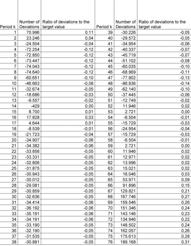
Table 2 The Deviation Numbers and The Ratios of Deviations To The Target Value

Period k

Number of Deviations

Ratio of deviations to the

target value Period k

Number of Deviations

Ratio of deviations to the target value 1 70.996 0,11 39 -30.226 -0,05 2 23.246 0,04 40 -29.572 -0,05 3 -24.504 -0,04 41 -34.954 -0,06 4 -72.254 -0,12 42 -40.337 -0,07 5 -72.850 -0,12 43 -45.719 -0,07 6 -73.447 -0,12 44 -51.102 -0,08 7 -74.043 -0,12 45 -60.035 -0,10 8 -74.640 -0,12 46 -68.969 -0,11 9 -60.651 -0,10 47 -77.902 -0,13 10 -46.663 -0,08 48 -86.836 -0,14 11 -32.674 -0,05 49 -62.140 -0,10 12 -18.686 -0,03 50 -37.445 -0,06 13 -9.557 -0,02 51 -12.749 -0,02 14 -429 0,00 52 11.946 0,02 15 8.700 0,01 53 2.721 0,00 16 17.828 0,03 54 -6.504 -0,01 17 4.644 0,01 55 -15.729 -0,03 18 -8.539 -0,01 56 -24.954 -0,04 19 -21.723 -0,04 57 -15.729 -0,03 20 -34.907 -0,06 58 -6.504 -0,01 21 -34.382 -0,06 59 2.721 0,00 22 -33.856 -0,05 60 11.946 0,02 23 -33.331 -0,05 61 12.971 0,02 24 -32.806 -0,05 62 13.996 0,02 25 -31.875 -0,05 63 15.021 0,02 26 -30.943 -0,05 64 16.046 0,03 27 -30.012 -0,05 65 53.971 0,09 28 -29.081 -0,05 66 91.896 0,15 29 -30.859 -0,05 67 129.821 0,21 30 -32.636 -0,05 68 167.746 0,27 31 -34.414 -0,06 69 159.546 0,26 32 -36.192 -0,06 70 151.346 0,24 33 -35.191 -0,06 71 143.146 0,23 34 -34.191 -0,06 72 134.946 0,22 35 -33.190 -0,05 73 148.502 0,24 36 -32.190 -0,05 74 162.057 0,26 37 -31.535 -0,05 75 175.613 0,28 38 -30.881 -0,05 76 189.168 0,31

(64)

56

Table 3 Total Inventory Levels Corresponding to Each Periods For The Current Recruitment System Period k Number of Deviations Period k Number of Deviations Period k Number of Deviations Period k Number of Deviations 1 547.750 20 653.653 39 648.973 58 625.250 2 595.500 21 653.128 40 648.318 59 616.025 3 643.250 22 652.603 41 653.701 60 606.800 4 691.000 23 652.077 42 659.083 61 605.775 5 691.597 24 651.552 43 664.466 62 604.750 6 692.193 25 650.621 44 669.848 63 603.725 7 692.790 26 649.690 45 678.782 64 602.700 8 693.386 27 648.758 46 687.715 65 564.775 9 679.398 28 647.827 47 696.649 66 526.850 10 665.409 29 649.605 48 705.582 67 488.925 11 651.421 30 651.383 49 680.887 68 451.000 12 637.432 31 653.160 50 656.191 69 459.200 13 628.304 32 654.938 51 631.496 70 467.400 14 619.175 33 653.938 52 606.800 71 475.600 15 610.047 34 652.937 53 616.025 72 483.800 16 600.918 35 651.937 54 625.250 73 470.245 17 614.102 36 650.936 55 634.475 74 456.689 18 627.286 37 650.282 56 643.700 75 443.134 19 640.469 38 649.627 57 634.475 76 429.578

(65)

57

Table 4 Total Inventory Levels Corresponding to Each Periods For Model With 12-Months Duration and Age 20.

Period k Number of Deviations Period k Number of Deviations Period k Number of Deviations Period k Number of Deviations 1 621,486 2 619,000 3 619,000 4 619,000 5 619,000 6 619,000 7 619,000 8 619,000 9 619,000 10 619,000 11 619,000 12 619,000 13 619,000 14 619,000 15 619,000 16 595,096 17 619,000 18 619,000 19 619,000 20 619,000 21 619,000 22 619,000 23 619,000 24 619,000 25 619,000 26 619,000 27 619,000 28 619,000 29 619,000 30 619,000 31 619,000 32 619,000 33 619,000 34 619,000 35 619,000 36 619,000 37 619,000 38 619,000 39 619,000 40 619,000 41 619,000 42 619,000 43 619,000 44 619,000 45 619,000 46 619,000 47 619,000 48 688,319 49 619,000 50 619,000 51 619,000 52 600,789 53 619,000 54 619,000 55 619,000 56 635,792 57 619,000 58 619,000 59 559,619 60 600,903 61 619,000 62 619,000 63 613,596 64 596,104 65 557,306 66 502,935 67 579,846 68 446,420 69 523,659 70 619,000 71 619,000 72 475,094 73 619,000 74 506,525 75 420,920 76 420,920

(66)

58

CHAPTER 5

SUMMARY AND CONCLUDING REMARKS

The current system results in a total deviation of 3.841.083 for the target inventory level of 619.000. This indicates a very high level of deviation for the system. The results of total inventories acquired from this system can be seen in Table 3 and the deviation numbers can be seen in Table 2. In comparison to the results of the current system, the results of the proposed model give a total deviation value of 1.373.865 for the same target value. This big change in the stability of the system to produce better results can be seen in Table 4. In our model the excess values can be controlled and the model reaches the target values or values nearest possible to the target level succeeding better deviation values in total. The number of values that are 619.000 are 58 and the number of values that are not 619.000 are only 18. If we take a modest range of (-,+)5% of the target value for the values of the current system, we see that only 19 values are in this range.

In the second phase, we run the model for zero deviations for the taken duration times. The model without the age flexibility gives the zero total of the deviations for a service duration of 12 months as 423000. The zero

(67)

59

deviation for the model when given the flexibility of the ages, is found as 600.000 for 12 months. This is a great change in the system’s stability. The zero total deviations of the durations of 15, 18 and 21 months are found as 612.000, 650.000 and 830.000 respectively.

Our model can be a solution to the problem of the fluctuating numbers of the human source even without the flexibility of varied ages of recruitment. The age flexibility if implemented increases the capacity of the model to create minimum deviation numbers for higher target inventory levels.

(68)

60

BIBLIOGRAPHY

1. Pekmezci, Arz, ‘Modeling The Officer Recruitment and Manpower Planning Process In Turkish Land Forces’, Master Thesis 2001 2. Gass, I., Saul, ‘The Army Manpower Long-Range Planning

System’, Operations Research, Vol. 36, No.1, January-February 1988 pp 5-17

3. Lagodimos, G., A., and Leopoulos, V., ‘ Greedy Heuristic

Algorithms For Manpower Shift Planning’, International Journal Of Production Economics Vol. 68, Issue 1, 30 October 2000, pp 95-106

4. Uğurateş, Can, ‘Geçmişten Günümüze Asker Alma’, Kara Kuvvetleri Dergisi October 2004, pp 22-26

5. Uzunçarşılı, İsmail Hakkı. 1984. Osmanlı Devleti Teşkilatından Kapıkulu Ocakları. Ankara: Türk Tarih Kurumu