For Permissions, please email: [email protected]
Advance Access publication on 30 July 2013 doi:10.1093/comjnl/bxt075
Recognizing Daily and Sports
Activities in Two Open Source Machine
Learning Environments Using
Body-Worn Sensor Units
Billur Barshan
∗and Murat Cihan Yüksek
Department of Electrical and Electronics Engineering, Bilkent University, Bilkent 06800, Ankara, Turkey ∗Corresponding author: [email protected]
This study provides a comparative assessment on the different techniques of classifying human activities performed while wearing inertial and magnetic sensor units on the chest, arms and legs. The gyroscope, accelerometer and the magnetometer in each unit are tri-axial. Naive Bayesian classifier, artificial neural networks (ANNs), dissimilarity-based classifier, three types of decision trees, Gaussian mixture models (GMMs) and support vector machines (SVMs) are considered. A feature set extracted from the raw sensor data using principal component analysis is used for classification. Three different cross-validation techniques are employed to validate the classifiers. A performance comparison of the classifiers is provided in terms of their correct differentiation rates, confusion matrices and computational cost. The highest correct differentiation rates are achieved with ANNs (99.2%), SVMs (99.2%) and a GMM (99.1%). GMMs may be preferable because of their lower computational requirements. Regarding the position of sensor units on the body, those worn on the legs are the most informative. Comparing the different sensor modalities indicates that if only a single sensor type is used, the highest classification rates are achieved with magnetometers, followed by accelerometers and gyroscopes. The study also provides a comparison between two commonly used open source machine learning environments (WEKA and PRTools) in terms of their functionality, manageability,
classifier performance and execution times.
Keywords: inertial sensors; accelerometer; gyroscope; magnetometer; wearable sensors; body sensor networks; human activity classification; classifiers; cross validation; machine learning environments;
WEKA; PRTools
Received 1 December 2012; revised 16 May 2013
Handling editor: Ethem Alpaydin
1. INTRODUCTION
With the rapid advances in micro electro-mechanical systems (MEMS) technology, the size, weight and cost of commer-cially available inertial sensors have decreased considerably over the last two decades [1]. Miniature sensor units that contain accelerometers and gyroscopes are sometimes complemented by magnetometers. Gyroscopes provide angular rate informa-tion around an axis of sensitivity, whereas accelerometers pro-vide linear or angular velocity rate information. There exist devices sensitive around a single axis, as well as two- and tri-axial devices. Tri-tri-axial magnetometers can detect the strength and direction of the Earth’s magnetic field as a vector quantity.
Until the 1990s, the use of inertial sensors was mostly limited to aeronautics and maritime applications because of the high cost associated with the high accuracy requirements. The avail-ability of lower cost, medium performance inertial sensors has opened up new possibilities for use (see Section 5).
The main advantages of inertial sensors is that they are self-contained, non-radiating, non-jammable devices that provide dynamic motion information through direct measurements in 3D. On the other hand, because they rely on internal sensing based on dead reckoning, errors at their output, when integrated to get position information, accumulate quickly and the position output tends to drift over time. The errors need to be modeled
1650 B. Barshan and M.C. Yüksek and compensated for, or reset from time to time when data from
external absolute sensing systems become available.
A recent application domain of inertial sensing is automatic recognition and monitoring of human activities. This is a research area with many challenges and one that has received tremendous interest, especially over the last decade. Several different approaches are commonly used for the purpose of activity monitoring. One such approach is to use sensing sys-tems fixed to the environment, such as vision syssys-tems with multiple video cameras [2–5]. Automatic recognition, represen-tation and analysis of human activities based on video images has had a high impact on security and surveillance, entertain-ment and personal archiving applications [6]. Reference [7] presents a comprehensive survey of the recent studies in this area, where in many, points of interest on the human body are pre-identified by placing visible markers such as light-emitting diodes on them and recording their positions by optical or magnetic imaging techniques. For example, [8] considers six activities, including falls, using the Smart infrared motion capture system. In [9], walking anomalies such as limping, dizziness and hemiplegia are detected using the same system. In [10], a number of activity models are defined for pose tracking and the pose space is explored using particle filtering. Using cameras fixed to the environment (or other ambient intelligence solutions) may be acceptable when activities are confined to certain parts of an indoor environment. If cameras are being used, the environment needs to be well illuminated and almost studio like. However, when activities are performed indoors and outdoors and involve going from place to place (e.g. commuting, shopping, jogging), fixed camera systems are not very practical because acquiring video data is difficult for long-term human motion analysis in such unconstrained environments. Recently, wearable camera systems have been proposed to overcome this problem [11]; however, the other disadvantages of camera systems still exist, such as occlusion effects, the correspondence problem, the high cost of processing and storing images, the need for using multiple camera projections from 3D to 2D, the need for camera calibration and cameras’ intrusions on privacy.
Using miniature inertial sensors that can be worn on the human body instead of employing sensor systems fixed to the environment has certain advantages. As stated in [12], ‘activity can best be measured where it occurs.’ Unlike visual motion capture systems that require a free line of sight, miniature inertial sensors can be flexibly used inside or behind objects without occlusion. 1D signals acquired from the multiple axes of inertial sensors can directly provide the required information in 3D. Wearable systems have the advantages of being with the user continuously and having low computation and power requirements. Earlier work on activity recognition using body-worn sensors is reviewed in detail in [13–16]. More focused literature surveys overviewing the areas of rehabilitation and biomechanics can be found in [17–19].
Camera systems and inertial sensors can be used comple-mentarily in many situations. In a number of studies, video cameras are used only as a reference for comparison with iner-tial sensor data [20–23], whereas in others, data from these two sensing modalities are integrated or fused [24,25]. Joint use of visual and inertial sensors has attracted considerable attention recently because of the robust performance and potentially wide application areas [26,27]. Fusing data from inertial sensors and magnetometers are also reported in the literature [21,28,29]. In this study, however, we have chosen to use a wearable sys-tem for activity recognition because of the various advantages mentioned above.
Activity spotting is a well-known subclass of activity
recognition tasks, where the starting and finishing points of well-defined activities are detected based on sequential data [30]. The classifiers used for activity spotting tasks can be divided into instance- and model-based classifiers, where the latter dominates the area. The advantages of instance-based classifiers are their simple structure, lower computational cost and power requirement, and their ability to deal with classes encountered for the first time during the test procedure [31]. On the other hand, in large-scale tasks, they cannot effec-tively handle changes in circumstances such as inter-subject variability.
Some of the problems with activity spotting are optimizing the number and configuration of the sensors and synchronizing them. Zappi et al. [32] propose sensor selection algorithms to develop energy-aware systems that deal with the power vs. accuracy trade-off. In another study, Ghasemzadeh [33] introduces the concept of ‘motion transcripts’ and proposes distributed algorithms to reduce power requirements. In [34], a method is developed for human full-body pose tracking and activity recognition based on the measurements of a few body-worn inertial orientation sensors. Reference [35] focuses on recognizing activities characterized by a hand motion and an accompanying sound for assembly and maintenance applications. Multi-user activities are addressed in [36]. The focus of [37] is to investigate inter-subject variability in a large dataset.
Within the context of the European research project OPPORTUNITY, mobile opportunistic activity and context recognition systems are developed [38]. Another European Union project (wearIT@work) focuses on developing a context-aware wearable computing system to support a production or maintenance worker by recognizing his/her actions and delivering timely information about activities performed [39]. A survey on wearable sensor systems for health monitoring and prognosis and the related research projects are presented in [40]. The main objective of the European Commission’s seventh framework project CONFIDENCE is the development and integration of innovative technologies to build a care system for the detection of short- and long-term abnormal events (such as falls) or unexpected behaviors that may be related to a
The Computer Journal
,
Vol. 57 No. 11, 2014health problem in the elderly [41]. This system aims to improve the chances of timely medical intervention and give the user a sense of security and confidence, thus prolonging his/her independence.
The classification techniques used in previous activity recognition research include threshold-based classification, hierarchical methods, decision trees (DTs), the k-nearest neighbor (k-NN) method, artificial neural networks (ANNs), support vector machines (SVMs), naive Bayesian (NB) model, Bayesian decision-making (BDM), Gaussian mixture models (GMMs), fuzzy logic and Markov models, among others. The use of these classifiers in various studies is detailed in an excellent review paper focused on activity classification [42]. In some studies, the outputs of several classifiers are combined to improve robustness; however, there exists only a small number of studies that compare two or more classifiers using exactly the same set of input feature vectors. These studies are summarized in Table1and provide some insight on the relative performance of the different classifiers. The comparisons in some of these studies, however, are based on only a small number of subjects (1–3). According to the results, although it appears that DTs and BDM provide the best accuracy, the reported performance differences may not always be statistically significant. Furthermore, contradictory studies exist [42]. It is stated in the same reference that ‘There is need for further studies investigating the relative performance of the range of different classifiers for different activities and sensor features and with large numbers of subjects. For example, techniques such as SVM and Gaussian mixture models show considerable promise but have not been applied to large datasets.’
Due to the lack of common ground among studies, results published so far are fragmented and difficult to compare, synthesize and build upon in a manner that allows broad conclusions to be reached. There is a rich variety in the number and type of sensors and subjects used, activities considered and methods employed for data acquisition. Usually, the modality and configuration of sensors are chosen without strong justification, depending more on what is convenient, rather than on performance optimization. The segmentation (windowing) of signals, the generation, selection and reduction of features, and the classifiers used also differ significantly. The variety of choices made in the studies since 1999 and their classification results are summarized in Table1. It would not be appropriate to make a direct comparison across the classification accuracies of the different studies, because there is no common ground between them. Comparisons among different classifiers should be made based on the same dataset in order to be fair and meaningful. Optimal pre-processing and feature selection may further enhance the performance of the classifiers, and sometimes can be more important than classifier choice. There is an urgent need for establishing a common framework so that the subject can be treated in a unified and systematic manner. Consensus on activity monitoring protocols,
the variables to report, a standardized set of activities and sensor configurations would be highly beneficial to this research area.
Many works have demonstrated 85–97% correct recognition of activities based on inertial sensor data; the main problem with many of these, however, is that the subjects are provided with instructions and highly supervised while performing the activities. A system that can recognize activities performed in an unsupervised and naturalistic way with correct recognition rates above 95% would be of high practical value and interest. Another important concern is the computational cost and real-time operability of recognition algorithms. Classifiers designed should be fast enough to provide a decision in real time or with only a very short delay. Therefore, in our opinion, performance criteria and design requirements for an activity recognition system are accuracies above 95% and (near) real-time operability.
This study follows up on our earlier work reported in [16], where miniature sensor units comprised inertial sensors and magnetometers fixed to different parts of the body are used for activity classification. The main contribution of the earlier article is that unlike previous studies, it uses many redundant sensors and extracts a variety of features from the sensor signals. Then, it performs an unsupervised feature transformation technique that allows considerable feature reduction through automatic selection of the most informative features. It also provides a systematic comparison between various classifiers used for human activity recognition based on a common dataset. It reports correct differentiation rates, confusion matrices and computational requirements of the classifiers.
In this study, we evaluate the performance of additional classification techniques and investigate sensor selection and configuration issues based on the previously acquired dataset. The classification methodology in terms of feature extraction and reduction and cross-validation techniques is the same as [16]. The classification techniques we compare in this study are the NB classifier, ANNs, the dissimilarity-based classifier (DBC), as well as three types of DTs, GMMs and SVMs. We ask subjects to perform the activities in their own way; we do not provide any instructions on how the activities should be performed. We present and compare the experimental results considering correct differentiation rates, confusion matrices, cross-validation techniques, machine learning environments and computational requirements. The main purpose and contribution of this article is to identify the best classifier, the most informative sensor type and/or combination, and the most suitable sensor configuration on the body. We consider all possible sensor-type combinations of the three sensor modalities (seven combinations altogether) and the position combinations of the given five positions on the body (31 combinations altogether). We note activities that are most confused with each other and compare the computational requirements of the classification techniques.
1652 B. Barshan and M.C. Yüksek
TABLE 1. A summary of the earlier studies on activity recognition indicating the wide variety of choices made. Activities
Reference Sensors No. type Subjects Classifiers used and classification rates
Aminian et al. [20] 1D acc (×2) 4 pos, mot 4M 1F Physical activity detection algorithm: 89.3%
Kern et al. [12] 3D acc (×12) 8 pos, mot 1M BDM: 85–89%
Mathie et al. [43] 3D acc (×1) 12 pos, mot, trans 19M 7F Hierarchical binary DT: 97.7%
Bao and Intille [44] 2D acc (×5) 20 pos, mot 13M 7F C4.5 DT: 84.26%, 1-NN: 82.70%, NB: 52.35%, DTable: 46.75% Allen et al. [45] 3D acc (×1) 8 pos, mot 2M 4F Adopted GMM: 92.2%, GMM: 91.3%, rule-based heuristics: 71.1% Pärkkä et al. [46] 3D acc, mag, other (total 23) 7 pos, mot 13M 3F Automatic DT: 86%, custom DT: 82%, ANN: 82%
Maurer et al. [47] 2D acc (×1), light sensor (×1) 6 pos, mot 6 C4.5 DT: 87.1% (wrist), NB and k-NN: not reported but both < 87.1% Pirttikangas et al. [48] 3D acc (×4), heart rate (×1) 17 pos, mot 9M 4F k-NN: 90.61%, ANN:∼81%
9 k-NN: 92.89%, ANN: 89.76%
Ermes et al. [49] 3D acc (×2), GPS (×1) 9 pos, mot 10M 2F Hybrid model: 89%, ANN: 87%, custom DT: 83%, automatic DT: 60%
Yang et al. [50] 3D acc (×1) 8 pos, mot 3M 4F ANN: 95.24%, k-NN: 87.18%
Luštrek and Kaluža [8] video tags (×12) 6 pos, mot 3 SVM: 96.3%, 3-NN: 95.3%, RF-T: 93.9%, bagging: 93.6%, Adaboost: 93.2%, C4.5 DT: 90.1%, RIPPER decision rules: 87.5%, NB: 83.9%
Tunçel et al. [51] single-axis gyro (×2) 8 mot 1M BDM: 99.3%, SVM: 98.4%, 1-NN: 98.2%,
DTW: 97.8%, LSM: 97.3%, ANN: 88.8% Khan et al. [52] 3D acc (×1) 15 pos, mot, trans 3M 3F Hierarchical recognizer (LDA+ANN): 97.9%
Altun et al. [16] 3D acc-gyro-mag unit (×5) 19 pos, mot 4M 4F BDM: 99.2%, SVM: 98.8%, 7-NN: 98.7%, DTW: 98.5%, ANN: 96.2%, LSM: 89.6%, RBA: 84.5%
Ayrulu and Barshan [53] single-axis gyro (×2) 8 mot 1M Features extracted by various wavelet families as input to ANN: 97.7% Lara et al. [54] 3D acc (×1), vital signs 5 pos, mot 7M 1F Additive Logistic Regression (ALR): 95.7%,
Bagging using ten J48 classifiers (BJ48): 94.24%
Bagging using ten Bayesian network classifiers (BBN): 88.33%
Aung et al. [55] video tags (Vicon system) 3 mot 8 Wavelet transform+ manifold embedding + GMM: 92%
3D acc (×2) (gait)
3 datasets
From left to right: the reference details, number and type of sensors [acc, accelerometer; gyro, gyroscope; mag, magnetometer; GPS, global positioning system; other, other type of sensors], number and type of activities classified [pos, posture; mot, motion; trans, transition], number of male (M) and female (F) subjects, the classifiers used and their correct differentiation rates sorted from maximum to minimum.
The
Computer
Journal
,
V ol. 57 No. 11, 2014The study also provides a comparison between two commonly used open source machine learning environments in terms of their functionality, manageability, classification performance and execution times of the classifiers employed. Our research group implemented the compared classification techniques in [16], whereas the classifiers considered in this study are provided in two open source environments in which a wide variety of choices are available. We use the Waikato environment for knowledge analysis (WEKA) and the pattern recognition toolbox (PRTools). WEKA is a Java-based collection of machine learning algorithms for solving data mining problems [56,57]. PRTools is a MATLAB-based toolbox for pattern recognition [58]. Since WEKA is executable in MATLAB, MATLAB is used as the master software to manage both environments.
The rest of this paper is organized as follows: Section 2 briefly describes the data acquisition, features used and activities performed. In Section 3, we state the classifiers used and outline the classification procedure. In Section 4, we present the experimental results of the performance of the classifiers, sensor selection and configuration, and execution times, and also compare the two machine learning environments. In Section 5, we note several application areas of activity recognition. We present our conclusions and suggest future research directions in Section 6.
2. DATA ACQUISITION, FEATURES AND ACTIVITIES
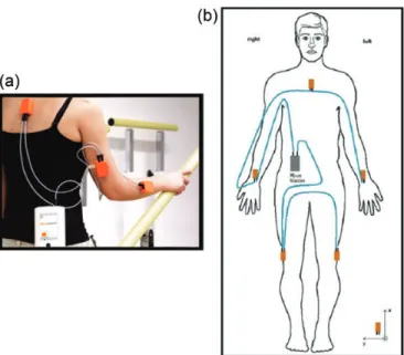
We use five MTx 3-DOF orientation trackers (Fig. 1), manufactured by Xsens Technologies [59]. Each MTx unit has a tri-axial accelerometer, a tri-axial gyroscope and a tri-axial magnetometer, thus the sensor units acquire 3D acceleration, rate of turn and the strength of the Earth’s magnetic field. Each motion tracker is programmed via an interface program called MT Manager to capture the raw or calibrated data with a sampling frequency of up to 512 Hz.
Accelerometers of two of the MTx trackers can sense up to ±5g and the other three can sense in the range of
±18g, where g = 9.80665 m/s2 is the standard gravity. All gyroscopes in the MTx unit can sense in the range of±1200◦/s angular velocities. The magnetometers measure the strength of the Earth’s magnetic field along three orthogonal axes and their vectoral combination provides the magnitude and the direction of the Earth’s magnetic north. In other words, the magnetometers function as a compass and can sense magnetic fields in the range of±75 μT.
We use all three types of sensor data in all three dimensions. The sensors are placed on five different points on the subject’s body, as depicted in Fig.2a. Since leg motions, in general, may produce larger accelerations, two of the±18g sensor units are placed on the sides of the knees (the right-hand side of the right knee (Fig.2b) and the left-hand side of the left knee), the remaining±18g unit is placed on the subject’s chest (Fig.2c), and the two±5g units on the wrists (Fig.2d).
The five MTx units are connected with 1 m cables to a device called the Xbus Master, which is attached to the subject’s belt (Fig.3a) and transmits data from the units to the receiver using a BluetoothTMconnection. The receiver is connected to a laptop computer via a USB port. Two of the five MTx units are directly connected to the Xbus Master and the remaining three are indirectly connected by wires through the other two (Fig.3b).
We classify 19 activities using body-worn miniature inertial sensor units: sitting (A1), standing (A2), lying on the back and on the right side (A3and A4), ascending and descending stairs (A5 and A6), standing still in an elevator (A7) and moving around in an elevator (A8), walking in a parking lot (A9), walking on a treadmill with a speed of 4 km/h in flat and 15◦ inclined positions (A10 and A11), running on a treadmill with a speed of 8 km/h (A12), exercising on a stepper (A13), exercising on a cross trainer (A14), cycling on an exercise bike in horizontal and vertical positions (A15and A16), rowing (A17), jumping (A18) and playing basketball (A19).
Each activity listed above is performed by eight volunteer subjects (four female, four male; ages 20–30) for 5 min. Details of the subject profiles are given in [60]. The experimental procedure was approved by Bilkent University Ethics Committee for Research Involving Human Subjects, and all subjects gave their informed written consent to participate
FIGURE 1. (a) MTx with sensor-fixed coordinate system overlaid and (b) MTx held between two fingers (both parts of the figure are reprinted
from [59]).
1654 B. Barshan and M.C. Yüksek
FIGURE 2. Positioning of the Xsens units on the body.
FIGURE 3. (a) MTx blocks and Xbus Master (the picture is reprinted
fromhttp://www.xsens.com/images/stories/products/PDF_Brochures/ mtx leaflet.pdf) and (b) connection diagram of MTx sensor blocks (body part of the figure is from http://www.answers.com/body breadths).
in the experiments. The subjects are asked to perform the activities in their own way, and are not restricted in this sense. While providing no instructions regarding the activities likely results in greater inter-subject variations in speed and amplitude than providing instructions does, we aim to mimic real-life situations, where people walk, run and exercise in their own fashion. The activities are performed at the Bilkent University Sports Hall, in Bilkent’s Electrical and Electronics Engineering Building, and in a flat outdoor area on campus. Sensor units
are calibrated to acquire data at 25 Hz sampling frequency. The 5-min signals are divided into 5-s segments, from which certain features are extracted. In this way, 480 (= 60 × 8) signal segments are obtained for each activity. Our dataset is publicly available at the UCI Machine Learning Repository (http://archive.ics.uci.edu/ml/).
After acquiring the signals as described above, we obtain a discrete-time sequence of Ns elements, represented as an
Ns× 1 vector s = [s1, s2, . . . , sNs]
T. For the 5-s time windows and the 25-Hz sampling rate, Ns = 125. The initial set of features we use before feature reduction is the minimum and maximum values, the mean value, variance, skewness, kurtosis, autocorrelation sequence and the peaks of the discrete Fourier transform (DFT) of s with the corresponding frequencies. Details on the calculation of these features, their normalization and the construction of the 1170× 1 feature vector for each of the 5-s signal segments are provided in [16,61]. A good feature set should minimize feature redundancy and show only small variations among repetitions of the same activities and across different subjects but should vary considerably between differ-ent activities. When correlations are considered, features with high intra-class but low inter-class correlations are preferable.
The initially large number of features is reduced from 1170 to 30 through principal component analysis (PCA) [62] because not all features are equally useful in discriminating between the activities [63]. After feature reduction, the resulting feature vector is an N×1 vector x = [x1, x2, . . . , xN]T, where N = 30 here. The reduced dimension of the feature vectors is determined by observing the eigenvalues of the covariance matrix of the 1170× 1 feature vectors, sorted in Fig.4a in descending order. The 30 eigenvectors corresponding to the largest 30 eigenvalues (Fig.4b) are used to form the transformation matrix, resulting in 30× 1 feature vectors. Scatter plots of the first five features selected by PCA are illustrated in Fig.5.
The Computer Journal
,
Vol. 57 No. 11, 20140 200 400 600 800 1000 1200 −0.5 0 0.5 1 1.5 2 2.5 3 3.5 4 4.5
eigenvalues in descending order
(a) 0 10 20 30 40 50 −0.5 0 0.5 1 1.5 2 2.5 3 3.5 4 4.5
first 50 eigenvalues in descending order
(b)
FIGURE 4. (a) All eigenvalues (1170) and (b) the first 50 eigenvalues of the covariance matrix sorted in descending order [16].
A1 A2 A3 A4 A5 A6 A7 A8 A9 A10 A11 A12 A13 A14 A15 A16 A17 A18 A19 4 2 0 –2 –4 feature 2 feature 1 4 2 0 –2 –4 feature 3 4 2 0 –2 –4 feature 4 4 2 0 –2 –4 feature 5 –6 –4 –2 0 2 4 feature 2 –6 –4 –2 0 2 4 feature 3 –6 –4 –2 0 2 4 feature 4 –6 –4 –2 0 2 4 (a) (b) (c) (d)
FIGURE 5. Scatter plots of the first five features selected by PCA.
3. CLASSIFICATION TECHNIQUES
We associate a class with each of the 19 activity types and label each feature vector x in the training set with the class that it belongs to. The total number of available feature vectors is constant but the way we distribute them between the training set and the test set depends on the cross-validation technique we employ (see Section 4.1). The test set is used to evaluate the performance of the classifier. The classification techniques we compare in this study are the NB classifier, ANNs, the DBC, three types of DTs, GMMs and SVMs. The three types of DTs are J48 trees (J48-T), NB trees (NB-T) and random forest trees
(RF-T). Details on the implementation of these classifiers and their parameters can be found in [61]. These are employed to classify the 19 different activities using the 30 features selected by PCA.
4. EXPERIMENTAL RESULTS 4.1. Cross-validation techniques
A total of 9120 (= 60 feature vectors × 19 activities × 8 subjects) feature vectors are available, each containing the
1656 B. Barshan and M.C. Yüksek 30 reduced features of the 5-s signal segments. In the training
and testing phases of the classification methods, we use the repeated random sub-sampling (RRSS), P -fold and L1O cross-validation techniques.
In RRSS, we divide the 480 feature vectors from each activity type randomly into two sets so that the first set contains 320 feature vectors (40 from each subject) and the second set contains 160 (20 from each subject). Therefore, two-thirds (6080) of the 9120 feature vectors are used for training and one third (3040) for testing. This is repeated 10 times and the resulting correct differentiation percentages are averaged. The disadvantage of this method is that some observations may never be selected in the testing or the validation phase, whereas others may be selected more than once. In other words, validation subsets may overlap.
In P -fold cross validation, the 9120 feature vectors are divided into P = 10 partitions, where the 912 feature vectors in each partition are randomly selected, regardless of the subject or class they belong to. One of the P partitions is retained as the validation set for testing, and the remaining P−1 partitions are used for training. The cross-validation process is then repeated
P times (the folds), so that each of the P partitions is used exactly once for validation. The P results from the folds are then averaged to produce a single estimate. The random partitioning is repeated 10 times and the average correct differentiation percentage is reported. The advantage of this validation method over RRSS is that all feature vectors are used for training and testing, and each feature vector is used for testing exactly once in each of the 10 runs.
In subject-based L1O cross validation, the 7980 (= 60 vectors× 19 activities × 7 subjects) feature vectors of seven of the subjects are used for training and the 1140 feature vectors of the remaining subject are used in turn for validation. This is repeated eight times, taking a different subject out for testing in each repetition. This way, the feature vector set of each subject is used once for testing (as the validation data). The eight correct classification rates are averaged to produce a single estimate. This is the same as P -fold cross validation, with P being equal to the number of subjects (P = 8), and all the feature vectors in the same partition being associated with the same subject.
Given the purpose of this study, once the system is trained, it is important to be able to correctly classify the activities of subjects encountered for the first time. The capability of the system in this respect is only measured by means of L1O cross validation. The RRSS and P -fold cross-validation approaches are valid only when the same subjects are to be used in the testing stage to evaluate the classifiers. The L1O scheme allows objective activity recognition as it treats the subjects as units, without having data samples from trials of the same subject contained within both training and testing partitions. Therefore, we consider the L1O results to be the most meaningful.
4.2. Correct differentiation rates
The classifiers used in this study are available in two commonly used open source machine learning environments: WEKA, a Java-based software [57]; and PRTools, a MATLAB toolbox [58]. The NB and ANN classifiers are tested in both environments to compare the implementations of the algorithms and the environments themselves. The SVMs and the three types of DTs are tested using WEKA. PRTools is used for testing the DBC and GMM for cases where the number of mixtures in the model varies from one to four.
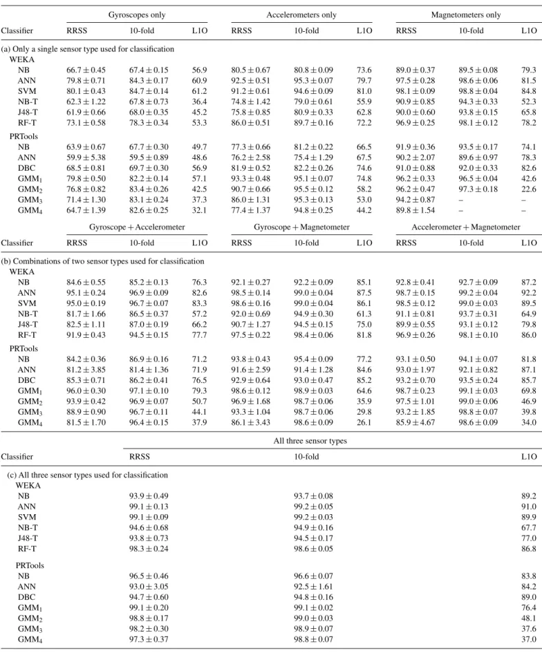
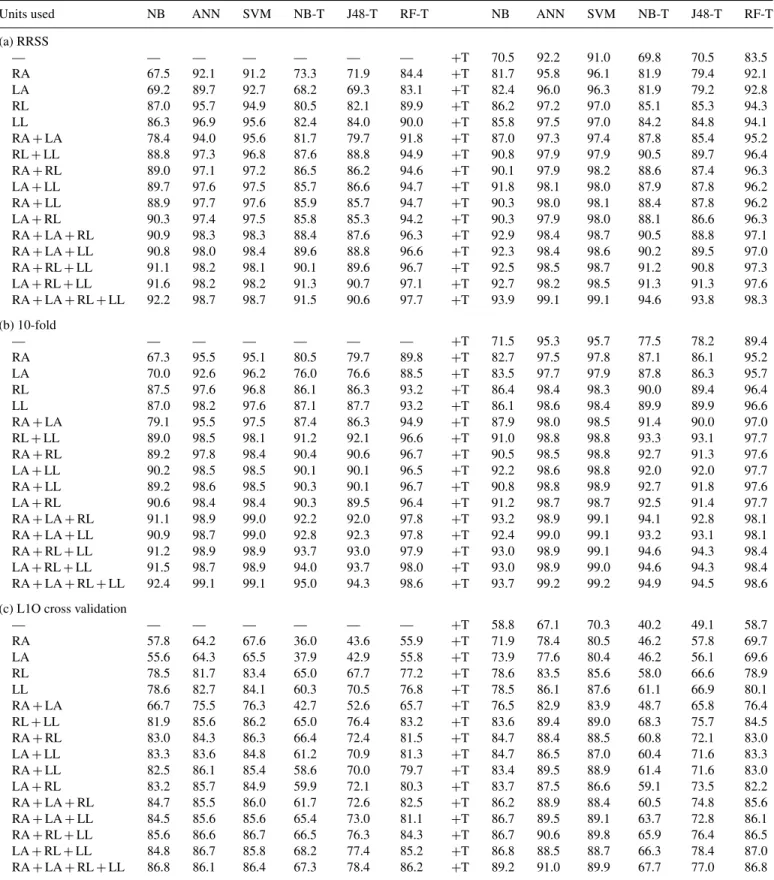
The classifiers are tested based on every combination of sensor type and a finite number of given sensor locations. First, data corresponding to all possible combinations of the three sensor types (seven combinations altogether) are used for classification; the correct differentiation rates and standard deviations over 10 runs are provided in Table2. Because L1O cross validation would give the same classification percentage if the complete cycle over the subject-based partitions were repeated, its standard deviation is zero. We also depict correct differentiation rates in the form of bar graphs (Fig. 6) for better visualization. Then, data corresponding to all possible combinations of sensor locations (31 combinations altogether) are used for the tests and the correct differentiation rates are shown in Tables3and4.
All three cross-validation techniques are used in the tests. We observe that 10-fold cross validation has the best performance, followed by RRSS, with slightly lower rates. This occurs because the former uses a larger fraction of the dataset for training (RRSS: 23, 10-fold: 109, L1O: 78 of the whole dataset). Subject-based L1O has the smallest rates in all cases because each subject performs the activities in a different manner. Outcomes obtained by implementing L1O indicate that the dataset should be sufficiently comprehensive in terms of the diversity of the subjects’ physical characteristics. It is expected that data from each additional subject with distinctive characteristics included in the training set will improve the correct classification rate of newly introduced feature vectors.
Among the DTs, RF-T is superior in all cases because it performs majority voting; each of the ten DTs casts a vote representing its decision and the class receiving the largest number of votes is considered to be the correct one. This method achieves an average correct differentiation rate of 98.6% for 10-fold cross validation when data from all sensors are used (Table2). NB-T seems to perform the worst of all DTs because of its feature independence assumption.
Generally, the best performance is expected from the ANNs and SVMs for classification problems involving multi-dimensional continuous feature vectors [64]. L1O cross-validation results for each sensor combination indicate their great capacity for generalization.As a consequence, they are less susceptible to overfitting than classifiers such as GMM. ANNs and SVMs are the best classifiers of the group and usually have slightly better performance than GMM1 (99.1%); both exhibit
The Computer Journal
,
Vol. 57 No. 11, 2014TABLE 2. Correct differentiation rates and the standard deviations based on all classifiers, cross-validation methods and both environments.
Gyroscopes only Accelerometers only Magnetometers only
Classifier RRSS 10-fold L1O RRSS 10-fold L1O RRSS 10-fold L1O
(a) Only a single sensor type used for classification WEKA NB 66.7± 0.45 67.4± 0.15 56.9 80.5± 0.67 80.8± 0.09 73.6 89.0± 0.37 89.5± 0.08 79.3 ANN 79.8± 0.71 84.3± 0.17 60.9 92.5± 0.51 95.3± 0.07 79.7 97.5± 0.28 98.6± 0.06 81.5 SVM 80.1± 0.43 84.7± 0.14 61.2 91.2± 0.61 94.6± 0.09 81.0 98.1± 0.09 98.8± 0.04 84.8 NB-T 62.3± 1.22 67.8± 0.73 36.4 74.8± 1.42 79.0± 0.61 55.9 90.9± 0.85 94.3± 0.33 52.3 J48-T 61.9± 0.66 68.0± 0.35 45.2 75.8± 0.85 80.9± 0.33 62.8 90.0± 0.60 93.8± 0.15 65.8 RF-T 73.1± 0.58 78.3± 0.34 53.3 86.0± 0.51 89.7± 0.16 72.2 96.9± 0.25 98.1± 0.12 78.2 PRTools NB 63.9± 0.67 67.7± 0.30 49.7 77.3± 0.66 81.2± 0.22 66.5 91.9± 0.36 93.5± 0.17 74.1 ANN 59.9± 5.38 59.5± 0.89 48.6 76.2± 2.58 75.4± 1.29 67.5 90.2± 2.07 89.6± 0.97 78.3 DBC 68.5± 0.81 69.7± 0.30 56.9 81.9± 0.52 82.2± 0.26 74.6 91.0± 0.88 92.0± 0.33 82.6 GMM1 79.8± 0.50 82.2± 0.14 57.1 93.3± 0.48 95.1± 0.07 74.8 96.2± 0.33 96.5± 0.04 42.6 GMM2 76.8± 0.82 83.4± 0.26 42.5 90.7± 0.66 95.5± 0.12 58.2 96.2± 0.47 97.3± 0.18 22.6 GMM3 71.4± 1.30 83.1± 0.24 37.3 86.0± 1.31 95.3± 0.13 53.0 94.2± 0.87 – – GMM4 64.7± 1.39 82.6± 0.25 32.1 77.4± 1.37 94.8± 0.25 44.2 89.8± 1.54 – –
Gyroscope+Accelerometer Gyroscope+ Magnetometer Accelerometer+ Magnetometer
Classifier RRSS 10-fold L1O RRSS 10-fold L1O RRSS 10-fold L1O
(b) Combinations of two sensor types used for classification WEKA NB 84.6± 0.55 85.2± 0.13 76.3 92.1± 0.27 92.2± 0.09 85.1 92.8± 0.41 92.7± 0.09 87.2 ANN 95.1± 0.24 96.9± 0.09 82.6 98.5± 0.14 99.0± 0.04 87.5 98.7± 0.15 99.2± 0.04 92.2 SVM 95.0± 0.19 96.7± 0.07 83.3 98.6± 0.16 99.0± 0.04 86.1 98.5± 0.12 99.0± 0.03 89.5 NB-T 81.7± 1.66 86.5± 0.37 57.2 92.0± 0.69 94.9± 0.30 61.3 91.1± 0.81 93.7± 0.31 64.9 J48-T 82.5± 1.11 87.0± 0.19 66.2 90.7± 1.27 94.5± 0.15 75.0 89.9± 0.55 93.1± 0.12 79.8 RF-T 91.9± 0.43 94.5± 0.15 77.7 97.5± 0.22 98.4± 0.06 81.8 96.9± 0.26 98.1± 0.10 86.0 PRTools NB 84.2± 0.36 86.9± 0.16 71.2 93.8± 0.43 95.4± 0.09 77.2 93.1± 0.50 94.1± 0.07 81.8 ANN 81.2± 3.85 81.4± 1.36 71.9 91.6± 2.59 91.4± 1.28 84.6 93.0± 1.97 92.1± 0.82 87.1 DBC 85.3± 0.71 86.2± 0.41 76.5 92.9± 0.64 93.0± 0.47 85.2 93.2± 0.70 93.5± 0.24 85.7 GMM1 96.0± 0.30 97.1± 0.10 79.3 98.6± 0.12 98.9± 0.03 64.6 98.7± 0.23 99.1± 0.03 69.8 GMM2 93.9± 0.42 96.9± 0.07 50.7 96.9± 1.68 98.7± 0.06 35.9 97.5± 1.01 99.0± 0.06 46.9 GMM3 88.9± 0.90 96.7± 0.11 44.1 93.3± 1.04 98.7± 0.06 29.8 93.2± 1.85 98.8± 0.07 39.8 GMM4 81.5± 1.70 96.4± 0.15 37.9 86.1± 3.43 98.6± 0.09 26.1 85.9± 4.67 98.6± 0.09 34.0
All three sensor types
Classifier RRSS 10-fold L1O
(c) All three sensor types used for classification WEKA NB 93.9± 0.49 93.7± 0.08 89.2 ANN 99.1± 0.13 99.2± 0.05 91.0 SVM 99.1± 0.09 99.2± 0.03 89.9 NB-T 94.6± 0.68 94.9± 0.16 67.7 J48-T 93.8± 0.73 94.5± 0.17 77.0 RF-T 98.3± 0.24 98.6± 0.05 86.8 PRTools NB 96.5± 0.46 96.6± 0.07 83.8 ANN 93.0± 3.05 92.5± 1.61 84.2 DBC 94.7± 0.60 94.8± 0.16 89.0 GMM1 99.1± 0.20 99.1± 0.02 76.4 GMM2 98.8± 0.17 99.0± 0.03 48.1 GMM3 98.2± 0.30 98.9± 0.07 37.6 GMM4 97.3± 0.37 98.8± 0.07 37.0
1658 B. Barshan and M.C. Yüksek 0 10 20 30 40 50 60 70 80 90 100 0 10 20 30 40 50 60 70 80 90 100 0 10 20 30 40 50 60 70 80 90 100 0 10 20 30 40 50 60 70 80 90 100 NB ANN SVM NB−T J48−T RF−T NB ANN SVM NB−T J48−T RF−T NB ANN SVM NB−T J48−T RF−T 0 10 20 30 40 50 60 70 80 90
100 Correct differentiation rates of the classifiers in WEKA (RRSS)
Correct differentiation rates of the classifiers in PRTools (RRSS)
Correct differentiation rates of the classifiers in WEKA (10-fold)
Correct differentiation rates of the classifiers in PRTools (10-fold)
Correct differentiation rates of the classifiers in WEKA (L1O)
Correct differentiation rates of the classifiers in PRTools (L1O)
gyro acc mag gyro + acc gyro + mag acc + mag gyro + acc + mag
gyro acc mag gyro + acc gyro + mag acc + mag gyro + acc + mag
gyro acc mag gyro + acc gyro + mag acc + mag gyro + acc + mag NB ANN DBC GMM1 GMM2 GMM3 GMM4 NB ANN DBC GMM1 GMM2 GMM3 GMM4 NB ANN DBC GMM1 GMM2 GMM3 GMM4 0 10 20 30 40 50 60 70 80 90 100 (a) (b) (c)
FIGURE 6. Comparison of classifiers and combinations of different sensor types in terms of correct differentiation rates using (a) RRSS, (b)
10-fold and (c) L1O cross validation. The sensor combinations represented by the different colors in the bar chart are identified in the legends. gyro, gyroscope; acc, accelerometer; mag, magnetometer.
The Computer Journal
,
Vol. 57 No. 11, 2014TABLE 3. All possible sensor unit combinations and the corresponding correct classification rates for the classifiers in WEKA using RRSS,
10-fold and L1O cross validation.
Units used NB ANN SVM NB-T J48-T RF-T NB ANN SVM NB-T J48-T RF-T
(a) RRSS — — — — — — — +T 70.5 92.2 91.0 69.8 70.5 83.5 RA 67.5 92.1 91.2 73.3 71.9 84.4 +T 81.7 95.8 96.1 81.9 79.4 92.1 LA 69.2 89.7 92.7 68.2 69.3 83.1 +T 82.4 96.0 96.3 81.9 79.2 92.8 RL 87.0 95.7 94.9 80.5 82.1 89.9 +T 86.2 97.2 97.0 85.1 85.3 94.3 LL 86.3 96.9 95.6 82.4 84.0 90.0 +T 85.8 97.5 97.0 84.2 84.8 94.1 RA+ LA 78.4 94.0 95.6 81.7 79.7 91.8 +T 87.0 97.3 97.4 87.8 85.4 95.2 RL+ LL 88.8 97.3 96.8 87.6 88.8 94.9 +T 90.8 97.9 97.9 90.5 89.7 96.4 RA+ RL 89.0 97.1 97.2 86.5 86.2 94.6 +T 90.1 97.9 98.2 88.6 87.4 96.3 LA+ LL 89.7 97.6 97.5 85.7 86.6 94.7 +T 91.8 98.1 98.0 87.9 87.8 96.2 RA+ LL 88.9 97.7 97.6 85.9 85.7 94.7 +T 90.3 98.0 98.1 88.4 87.8 96.2 LA+ RL 90.3 97.4 97.5 85.8 85.3 94.2 +T 90.3 97.9 98.0 88.1 86.6 96.3 RA+ LA + RL 90.9 98.3 98.3 88.4 87.6 96.3 +T 92.9 98.4 98.7 90.5 88.8 97.1 RA+ LA + LL 90.8 98.0 98.4 89.6 88.8 96.6 +T 92.3 98.4 98.6 90.2 89.5 97.0 RA+ RL + LL 91.1 98.2 98.1 90.1 89.6 96.7 +T 92.5 98.5 98.7 91.2 90.8 97.3 LA+ RL + LL 91.6 98.2 98.2 91.3 90.7 97.1 +T 92.7 98.2 98.5 91.3 91.3 97.6 RA+ LA + RL + LL 92.2 98.7 98.7 91.5 90.6 97.7 +T 93.9 99.1 99.1 94.6 93.8 98.3 (b) 10-fold — — — — — — — +T 71.5 95.3 95.7 77.5 78.2 89.4 RA 67.3 95.5 95.1 80.5 79.7 89.8 +T 82.7 97.5 97.8 87.1 86.1 95.2 LA 70.0 92.6 96.2 76.0 76.6 88.5 +T 83.5 97.7 97.9 87.8 86.3 95.7 RL 87.5 97.6 96.8 86.1 86.3 93.2 +T 86.4 98.4 98.3 90.0 89.4 96.4 LL 87.0 98.2 97.6 87.1 87.7 93.2 +T 86.1 98.6 98.4 89.9 89.9 96.6 RA+ LA 79.1 95.5 97.5 87.4 86.3 94.9 +T 87.9 98.0 98.5 91.4 90.0 97.0 RL+ LL 89.0 98.5 98.1 91.2 92.1 96.6 +T 91.0 98.8 98.8 93.3 93.1 97.7 RA+ RL 89.2 97.8 98.4 90.4 90.6 96.7 +T 90.5 98.5 98.8 92.7 91.3 97.6 LA+ LL 90.2 98.5 98.5 90.1 90.1 96.5 +T 92.2 98.6 98.8 92.0 92.0 97.7 RA+ LL 89.2 98.6 98.5 90.3 90.1 96.7 +T 90.8 98.8 98.9 92.7 91.8 97.6 LA+ RL 90.6 98.4 98.4 90.3 89.5 96.4 +T 91.2 98.7 98.7 92.5 91.4 97.7 RA+ LA + RL 91.1 98.9 99.0 92.2 92.0 97.8 +T 93.2 98.9 99.1 94.1 92.8 98.1 RA+ LA + LL 90.9 98.7 99.0 92.8 92.3 97.8 +T 92.4 99.0 99.1 93.2 93.1 98.1 RA+ RL + LL 91.2 98.9 98.9 93.7 93.0 97.9 +T 93.0 98.9 99.1 94.6 94.3 98.4 LA+ RL + LL 91.5 98.7 98.9 94.0 93.7 98.0 +T 93.0 98.9 99.0 94.6 94.3 98.4 RA+ LA + RL + LL 92.4 99.1 99.1 95.0 94.3 98.6 +T 93.7 99.2 99.2 94.9 94.5 98.6
(c) L1O cross validation
— — — — — — — +T 58.8 67.1 70.3 40.2 49.1 58.7 RA 57.8 64.2 67.6 36.0 43.6 55.9 +T 71.9 78.4 80.5 46.2 57.8 69.7 LA 55.6 64.3 65.5 37.9 42.9 55.8 +T 73.9 77.6 80.4 46.2 56.1 69.6 RL 78.5 81.7 83.4 65.0 67.7 77.2 +T 78.6 83.5 85.6 58.0 66.6 78.9 LL 78.6 82.7 84.1 60.3 70.5 76.8 +T 78.5 86.1 87.6 61.1 66.9 80.1 RA+ LA 66.7 75.5 76.3 42.7 52.6 65.7 +T 76.5 82.9 83.9 48.7 65.8 76.4 RL+ LL 81.9 85.6 86.2 65.0 76.4 83.2 +T 83.6 89.4 89.0 68.3 75.7 84.5 RA+ RL 83.0 84.3 86.3 66.4 72.4 81.5 +T 84.7 88.4 88.5 60.8 72.1 83.0 LA+ LL 83.3 83.6 84.8 61.2 70.9 81.3 +T 84.7 86.5 87.0 60.4 71.6 83.3 RA+ LL 82.5 86.1 85.4 58.6 70.0 79.7 +T 83.4 89.5 88.9 61.4 71.6 83.0 LA+ RL 83.2 85.7 84.9 59.9 72.1 80.3 +T 83.7 87.5 86.6 59.1 73.5 82.2 RA+ LA + RL 84.7 85.5 86.0 61.7 72.6 82.5 +T 86.2 88.9 88.4 60.5 74.8 85.6 RA+ LA + LL 84.5 85.6 85.6 65.4 73.0 81.1 +T 86.7 89.5 89.1 63.7 72.8 86.1 RA+ RL + LL 85.6 86.6 86.7 66.5 76.3 84.3 +T 86.7 90.6 89.8 65.9 76.4 86.5 LA+ RL + LL 84.8 86.7 85.8 68.2 77.4 85.2 +T 86.8 88.5 88.7 66.3 78.4 87.0 RA+ LA + RL + LL 86.8 86.1 86.4 67.3 78.4 86.2 +T 89.2 91.0 89.9 67.7 77.0 86.8
The last six columns display the results when the torso unit is added (+T) to the sensor combination given in the first column.
1660 B. Barshan and M.C. Yüksek
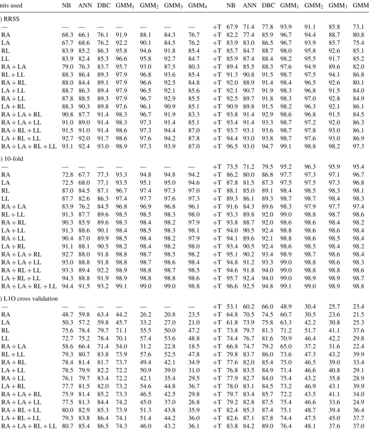
TABLE 4. All possible sensor unit combinations and the corresponding correct classification rates for the classifiers in PRTools using RRSS,
10-fold and L1O cross validation.
Units used NB ANN DBC GMM1 GMM2 GMM3 GMM4 NB ANN DBC GMM1 GMM2 GMM3 GMM4
(a) RRSS — — — — — — — — +T 67.9 71.4 77.8 93.9 91.1 85.8 73.1 RA 68.3 66.1 76.1 91.9 88.1 84.3 76.7 +T 82.2 77.4 85.9 96.7 94.4 88.7 80.8 LA 67.7 68.6 76.2 92.2 90.1 84.5 76.2 +T 83.9 83.0 86.5 96.7 93.9 85.7 75.4 RL 83.9 85.2 86.3 95.8 94.6 91.8 85.4 +T 85.7 84.7 88.7 98.0 95.8 92.6 85.1 LL 83.9 82.4 85.3 96.6 95.8 92.7 84.7 +T 85.9 87.4 88.4 98.2 95.5 91.7 85.2 RA+ LA 79.0 76.3 83.7 95.7 93.0 87.5 80.3 +T 89.4 85.5 88.3 97.6 94.9 89.6 82.0 RL+ LL 88.3 86.4 89.3 97.9 96.8 93.6 85.4 +T 91.3 90.8 91.5 98.7 97.5 94.1 86.8 RA+ RL 88.0 84.4 89.1 97.9 96.6 92.5 84.8 +T 92.0 88.9 91.4 98.4 96.5 92.6 80.1 LA+ LL 88.7 86.3 89.4 97.9 96.5 92.1 85.6 +T 92.1 90.7 91.9 98.3 96.8 91.5 84.0 RA+ LL 87.8 88.5 89.3 97.9 96.7 92.9 85.5 +T 92.5 89.7 91.8 98.3 97.0 92.8 84.9 LA+ RL 88.3 90.3 89.8 97.6 96.1 90.9 85.1 +T 90.9 89.8 91.5 98.2 96.3 92.1 86.1 RA+ LA + RL 90.8 87.7 91.4 98.3 96.7 91.9 83.3 +T 93.8 91.4 92.9 98.6 96.8 91.5 84.5 RA+ LA + LL 91.0 89.0 91.4 98.3 97.3 91.4 85.1 +T 93.4 91.4 93.3 98.7 97.2 92.0 86.3 RA+ RL + LL 91.5 91.0 91.4 98.6 97.3 94.4 87.0 +T 93.7 93.1 93.6 98.7 97.8 93.0 86.1 LA+ RL + LL 92.7 92.0 91.7 98.6 97.6 94.2 87.8 +T 94.4 93.0 93.8 98.7 97.6 93.0 86.9 RA+ LA + RL + LL 93.1 92.4 93.0 98.9 97.3 93.9 87.0 +T 96.5 93.0 94.7 99.1 98.8 98.2 97.3 (b) 10-fold — — — — — — — — +T 73.5 71.2 79.5 95.2 96.3 95.9 95.4 RA 72.8 67.7 77.3 93.3 94.8 94.8 94.2 +T 86.2 80.0 86.8 97.7 97.3 97.1 96.7 LA 72.5 68.0 77.1 93.5 95.1 95.0 94.6 +T 87.8 81.5 87.3 97.5 97.5 97.3 96.8 RL 87.0 84.5 87.1 96.7 97.4 97.3 97.0 +T 88.1 85.0 89.1 98.4 98.5 98.3 98.1 LL 87.7 82.6 86.3 97.4 97.7 97.6 97.3 +T 89.3 86.1 89.3 98.7 98.7 98.4 98.3 RA+ LA 83.9 76.2 84.5 96.8 96.9 96.8 96.1 +T 91.6 84.3 89.6 98.3 97.9 97.7 97.4 RL+ LL 91.3 87.7 89.6 98.5 98.5 98.3 98.0 +T 93.3 89.8 92.0 99.0 98.8 98.7 98.6 RA+ RL 90.3 85.9 89.6 98.3 98.4 98.2 97.9 +T 93.8 88.7 92.0 98.6 98.6 98.4 98.2 LA+ LL 91.3 88.6 90.1 98.4 98.5 98.3 98.1 +T 94.0 90.5 92.4 98.8 98.6 98.6 98.4 RA+ LL 90.4 87.0 89.9 98.5 98.4 98.2 97.9 +T 94.1 89.6 92.1 98.8 98.6 98.5 98.4 LA+ RL 91.1 88.1 90.5 98.2 98.4 98.2 98.0 +T 93.4 90.5 92.4 98.6 98.5 98.4 98.2 RA+ LA + RL 92.7 88.0 91.8 98.8 98.7 98.5 98.2 +T 95.1 90.2 93.4 98.9 98.7 98.6 98.4 RA+ LA + LL 93.0 88.8 91.8 98.8 98.7 98.6 98.4 +T 94.8 91.2 93.3 99.0 98.8 98.6 98.3 RA+ RL + LL 93.3 89.4 92.2 98.9 98.8 98.7 98.5 +T 94.6 91.8 94.0 99.0 98.8 98.8 98.6 LA+ RL + LL 94.3 88.8 91.9 98.9 98.8 98.8 98.6 +T 95.7 92.4 94.0 99.0 98.9 98.9 98.7 RA+ LA + RL + LL 94.4 91.5 93.2 99.1 99.0 99.0 98.8 +T 96.6 92.5 94.8 99.1 99.0 98.9 98.8
(c) L1O cross validation
— — — — — — — — +T 53.1 60.2 66.0 48.9 30.4 25.7 23.4 RA 48.7 59.8 63.4 44.2 26.2 20.8 23.5 +T 64.8 70.5 74.5 60.7 30.5 23.6 21.5 LA 50.3 57.2 59.8 45.7 33.2 27.0 21.0 +T 61.8 73.9 75.8 63.3 42.2 30.8 25.3 RL 75.6 78.4 79.7 71.1 55.5 50.0 47.2 +T 73.8 79.7 81.3 71.2 51.7 41.1 37.6 LL 72.7 75.2 78.4 70.1 57.4 53.6 48.8 +T 74.4 76.7 81.6 70.9 46.4 42.2 29.8 RA+ LA 58.6 66.4 71.4 54.0 31.2 22.8 18.5 +T 66.8 74.7 79.2 65.0 37.2 31.6 22.4 RL+ LL 79.3 80.7 83.8 73.9 57.6 52.5 47.8 +T 79.8 83.7 86.0 73.6 47.3 43.2 39.9 RA+ RL 78.4 81.4 81.7 73.7 49.4 42.1 34.9 +T 77.6 82.0 85.4 75.0 46.5 39.0 33.4 LA+ LL 78.5 79.9 82.2 72.2 50.9 39.0 31.0 +T 76.8 83.5 84.9 71.4 46.6 40.8 29.1 RA+ LL 76.1 79.7 83.4 72.2 42.1 35.4 29.5 +T 77.9 82.7 84.0 75.4 43.2 35.8 28.9 LA+ RL 77.7 81.5 82.0 73.2 54.6 44.8 36.7 +T 78.0 83.1 84.5 73.2 46.9 43.1 39.9 RA+ LA + RL 75.9 81.4 85.2 73.3 46.5 42.5 29.8 +T 79.7 83.4 85.7 72.2 43.5 41.1 34.0 RA+ LA + LL 77.5 81.3 84.4 74.2 45.0 37.0 26.8 +T 79.2 82.8 87.5 75.4 46.6 33.6 24.9 RA+ RL + LL 80.0 82.9 85.3 73.9 51.3 43.8 35.9 +T 82.4 85.3 87.4 75.1 48.7 39.4 36.4 LA+ RL + LL 79.3 83.8 86.4 74.1 51.4 44.2 36.0 +T 82.6 87.1 87.8 74.4 47.5 45.0 37.7 RA+ LA + RL + LL 80.7 85.4 86.5 74.3 46.0 43.2 36.1 +T 83.8 84.2 89.0 76.4 48.1 37.6 37.0
The last six columns display the results when the torso unit is added (+T) to the sensor combination given in the first column.
The Computer Journal
,
Vol. 57 No. 11, 201499.2% for 10-fold cross validation when the feature vectors extracted by the joint use of all sensor types are employed for classification (Table2c). L1O cross-validation accuracies are significantly better than GMM1.
The ANN implemented in PRTools does not perform as well as the one in WEKA. Before training an ANN with the back-propagation algorithm, it should be properly initialized. The most important parameters to initialize are the learning and momentum constants and the initial values of the connection weights. PRTools does not allow the user to choose the values of these two constants even though they play a crucial role in updating the weights. Without proper values, it is difficult to provide the ANN with suitable initial weights; therefore, the correct differentiation rates of the ANN implemented in PRTools do not reflect the true potential of the classifier.
Considering the outcomes obtained based on 10-fold cross validation and each sensor combination, it is difficult to determine the number of mixture components to be used in the GMM method. The average correct differentiation rates are quite close to each other for GMMs with one, two and three components (GMM1, GMM2 and GMM3). However, in the case of RRSS, and especially for L1O cross validation, the rates decrease rapidly as the number of components in the mixture increases. This may occur because the dataset is not sufficiently large to train GMMs with more than one component: it is observed in Table2a that GMM3and GMM4could not be trained due to insufficient data when only magnetometers are used. Another reason could be overfitting [65]. While multiple Gaussian estimators are exceptionally complex for classifying training patterns, they are unlikely to result in acceptable classification of novel patterns. Low differentiation rates of the GMM for L1O in all cases support the overfitting condition. Despite the lower rates obtained with this method for the L1O case, however, it is the third-best classifier, with a 99.1% average correct differentiation rate based on 10-fold cross validation when data from all sensor types are used (Table2c).
Comparing the classification results based on the different sensor combinations indicates that if only a single sensor type is used, the best correct differentiation rates are obtained by magnetometers, followed by accelerometers and gyroscopes. For a considerable number of classifiers, the rates achieved by using the magnetometer data alone are higher than those obtained by using the data of the other two sensors together. It can be observed in Fig. 6 that for almost all classifiers and all cross-validation techniques, the magnetometer bar is higher than the gyro+accelerometer bar, except for the GMM, ANN and NB-T used in L1O cross validation. It can be stated that the features extracted from the magnetometer data, which slowly vary in nature, may not be sufficiently diverse for training the GMM classifier. This statement is supported by the results provided in Table 2a, where we see that GMM3 and GMM4cannot be trained with magnetometer-based feature vectors. The best performance (98.8%) based on magnetometer data is achieved with the SVM using 10-fold cross validation
(Table2a). Outcomes of the combination of gyroscopes with the other two sensors are usually worse than the combination of accelerometer and magnetometer. The joint use of all three types of data provides the best classification performance, as expected.
When all 31 combinations of the sensor units at different positions on the body are considered, GMM usually has the best performance for all cross-validation techniques, except L1O (Tables 3 and 4). In L1O cross validation, ANNs and SVMs are superior. In 10-fold cross validation (Table 4b), correct differentiation rates achieved with GMM2are better than GMM1 in the tests where a single unit or the combination of two units is used. The units placed on the legs (RL and LL) seem to be the most informative. Comparing the cases where feature vectors are extracted from single sensor-unit data, it is observed that the highest correct classification rates are achieved with these two units. They also improve the performance of the combinations in which they are included.
4.3. Confusion matrices
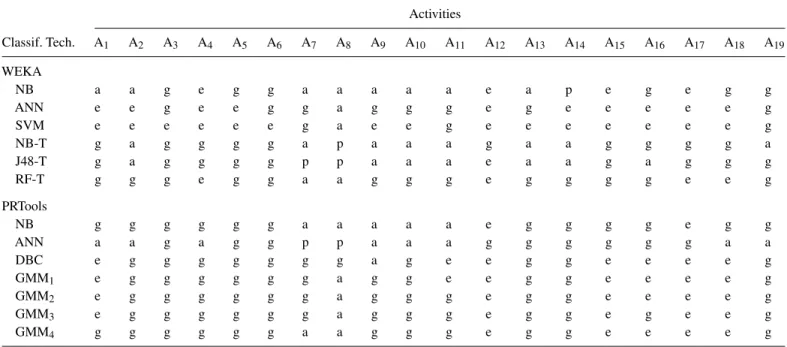
Based on the confusion matrices of the different techniques presented in [61], the activities that are most confused with each other are A7and A8. Since both are performed in an elevator, the corresponding signals contain similar segments. A2and A7, A13 and A14, as well as A9, A10and A11are also confused from time to time for similar reasons. A12and A17are the two activities that are almost never confused. The results based on the confusion matrices are summarized in Table5to report the performance of the classifiers in distinguishing each activity. The feature vectors that belong to A3, A4, A5, A6, A12, A15, A17 and A18 are classified with above-average performance by all classifiers. The remaining feature vectors cannot be classified well by some classifiers.
4.4. Comparison of the two machine learning environments
In comparing the two machine learning environments in this study, algorithms implemented in WEKA appear to be more robust to parameter changes than those in PRTools. In addition, WEKA is easier to work with because of its graphical user interface (GUI), which displays detailed descriptions of the algorithms along with their references and parameters when needed. PRTools does not have a GUI and the descriptions of the algorithms given in the references are insufficient. However, PRTools is more compatible with MATLAB. Nevertheless, both machine learning environments are powerful tools for pattern recognition.
The implementation of the same algorithm in WEKA and PRTools may not turn out to be exactly the same; for instance, the correct differentiation rates obtained with the NB and ANN classifiers do not match. Higher rates are achieved
1662 B. Barshan and M.C. Yüksek
TABLE 5. The performances of the classifiers in distinguishing different activity types.
Activities Classif. Tech. A1 A2 A3 A4 A5 A6 A7 A8 A9 A10 A11 A12 A13 A14 A15 A16 A17 A18 A19 WEKA NB a a g e g g a a a a a e a p e g e g g ANN e e g e e g g a g g g e g e e e e e g SVM e e e e e e g a e e g e e e e e e e g NB-T g a g g g g a p a a a g a a g g g g a J48-T g a g g g g p p a a a e a a g a g g g RF-T g g g e g g a a g g g e g g g g e e g PRTools NB g g g g g g a a a a a e g g g g e g g ANN a a g a g g p p a a a g g g g g g a a DBC e g g g g g g g a g e e g g e e e e g GMM1 e g g g g g g a g g e e g g e e e e g GMM2 e g g g g g g a g g g e g g e e e e g GMM3 e g g g g g g a g g g e g g e g e e g GMM4 g g g g g g a a g g g e g g e e e e g
These results are based on the confusion matrices given in [61], according to the number of feature vectors of a certain activity that the classifier correctly classifies out of 480 [p, poor (<400); a, average (400–459); g, good (460–479); e, excellent (exactly 480)].
with NB implemented in PRTools because the distribution of each feature is estimated using histograms; WEKA uses a normal distribution to estimate the PDFs. Considering the ANN classifier, PRTools does not allow the user to set the values for the learning and momentum constants that play a crucial role in updating the connection weights. Therefore, the ANN implemented in PRTools does not perform as well as the one in WEKA.
4.5. Comparison with earlier studies
To the best of our knowledge, other than the results of our research group, the highest reported correct classification rate in earlier studies (97.9%) is achieved through a hierarchical recognizer based on 3D accelerometer data (see Table1) [52]. However, this result is not directly comparable with ours or other results because of the lack of common ground, as explained in Section 1. The previously reported results by our research group indicate that BDM provides a correct classification rate of 99.2% with relatively small computational cost and storage requirements [16]. In this study, the same rate of 99.2% is achieved with ANN and SVM in WEKA. This is higher than those reported for the same two classifiers in [16] by 3 and 0.4% (for 10-fold) and 16.7 and 2.3% (for L1O), respectively. These differences arise both from the implementation of the algorithms and the variation in the random distribution of the feature vectors in the partitions obtained by using RRSS and 10-fold cross validation. The high classification rates achieved with BDM and GMM1in these studies illustrate the high estimation efficiency
of multi-variate Gaussian models for activity recognition tasks. However, these models may not be suitable when subject-based L1O cross validation is employed; for occasions where high generalization accuracy is required, they need to be replaced with ANNs or SVMs.
Although both are based on the Bayesian approach, the NB classifier is much simpler than BDM because of its feature independence assumption. The average correct classification rates previously reported by our group for BDM using RRSS and 10-fold cross-validation techniques are 99.1 and 99.2%, respectively [16], whereas these rates drop to 96.5 and 96.6% for NB in this study (Table 2c). Thus, the NB assumption of independence (given the class), though simplifying, is not necessarily a better choice.
4.6. Computational considerations
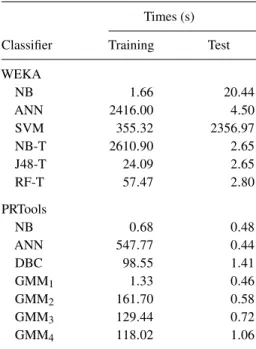
We compare the performances of the classifiers implemented in the two machine learning environments in terms of their execution times. The master software MATLAB is run on a computer with a Pentium (R) Dual-Core CPU E520 at a clock frequency of 2.50 GHz, 2.00 GB of RAM, and operated with Microsoft Windows XP Home Edition. Execution times are measured separately for the training and test stages and are provided in Table 6. The results correspond to the time it takes to complete a full L1O cross-validation cycle. In other words, each classifier is run eight times for all subjects and the total time of the complete cycle for each classifier is recorded. Given that these classifiers are to be
The Computer Journal
,
Vol. 57 No. 11, 2014TABLE 6. Execution times of training and test
steps for all classification techniques based on the full cycle of the L1O cross-validation method and both environments.
Times (s)
Classifier Training Test
WEKA NB 1.66 20.44 ANN 2416.00 4.50 SVM 355.32 2356.97 NB-T 2610.90 2.65 J48-T 24.09 2.65 RF-T 57.47 2.80 PRTools NB 0.68 0.48 ANN 547.77 0.44 DBC 98.55 1.41 GMM1 1.33 0.46 GMM2 161.70 0.58 GMM3 129.44 0.72 GMM4 118.02 1.06
used in real time, it is desirable to keep the test times at a minimum.
Considering WEKA, test times can be misleading because apart from the time consumed for calculating the correct differentiation rate, several other performance criteria, such as various error parameters and confusion matrices, are calculated during the test step. The time consumed for those calculations are included in the total time (given in Table6) but the actual test times should be much shorter. In contrast, computational times in PRTools are quite consistent. Therefore, it is not possible to compare these two environments in terms of their classification speed.
Among the DTs, NB-T has the longest training time (because an NB classifier must be trained for every leaf node), whereas J48-T has the shortest. There is hardly any difference between DT test times. Therefore, taking into account its high classification accuracy, RF-T seems to be a good compromise. DTs perform better than the other classifiers in terms of their testing durations in WEKA.
The training and testing of the ANNs and SVMs, identified to be the best in terms of classification accuracy, take much longer than the other classifiers. SVMs require the longest testing time because they use a Gaussian kernel for mapping and consider all possible pairwise combinations of classes. Therefore, ANNs are preferable to SVMs. On the other hand, GMM1, with its short training and test time requirements, could be considered (except for the L1O case, where the choice would be ANNs or SVMs). The DBC, with its moderate correct classification rates
and longest test time, is not preferable among the classifiers used in PRTools.
5. APPLICATION AREAS
The human activity monitoring and classification techniques presented in this work can be utilized in diverse areas. Those related to medicine include remote diagnosis and treatment of disorders [66], preventive care, chronic disease management (e.g. Parkinson’s disease, multiple sclerosis, epilepsy, gait dis-orders), tele-rehabilitation [67], tele-surgery [68] and biome-chanics [18,69]. In tele-rehabilitation, proper performance of daily physical therapy exercises assigned, for example, after a stroke or surgery, can be remotely monitored and proper feed-back provided to the patient and doctor [70]. Further, abnormal behaviors and emergency situations such as falls or changes in vital signs can be detected almost instantly and timely medical intervention thus provided [71–73]. Remote monitoring of the physically or mentally disabled, the elderly and children can be achieved indoors and outdoors [43] and cognitive assistance provided when needed. An emerging application area is behav-ioral medicine, where body-worn inertial sensors can be used for metabolic energy expenditure estimation, diet and medicine monitoring and management, lifestyle coaching and improving personal fitness and wellbeing. For example, a fitness applica-tion could use real-time activity informaapplica-tion to encourage users to perform opportunistic activities.
Wearable sensor technology can be used in the areas of physical education, training, sports science [49] and performing arts to guide the individual to improve his/her skills and prevent injury. The best and most ergonomic way to use a tool or a machine can be taught to workers in complex industrial environments [46]. In animation and film making, wearable sensors could be used in a complementary fashion with cameras to develop realistic animated models. In entertainment, more realistic and appealing video games can be produced when body-worn inertial sensors are integrated into the game and motion classifiers are embedded for recognizing a player’s moves [74,75].
Automatic recognition of the emotional qualities (aspects) of body movements from captured motion data is a recently developing area worth mentioning [76]. Body posture and bodily expressions may provide important clues on people’s emotional and mental states. In many applications (e.g. rehabilitation, human-robot interaction, cooperation of robots, computer games, military activities), joint knowledge of the type of activity performed and the emotional state under which it is performed can facilitate the intervention to affect people’s cognitive and affective processes. Combining the work proposed in this paper with that in [77] would, for example, allow an automatic adaptation of the game for either entertainment purpose or for physical rehabilitation.
Today’s advanced cell phone industry provides many opportunities as well; for example, developing applications for
1664 B. Barshan and M.C. Yüksek smart phones using embedded 3D inertial sensors to monitor
daily activities would be highly beneficial to the users [78].
6. CONCLUSIONS AND FUTURE WORK
We present the results of a comparative study where the features extracted from miniature inertial sensor and magnetometer signals are used for classifying human activities. The main contributions of this study are (i) to compare and identify the classifier(s) that satisfy the performance requirements and design criteria for an activity recognition system on a common basis, (ii) to determine the most informative sensor modality and/or combination and (iii) to determine the most suitable wearable sensor configuration. We compare a number of classifiers based on the same dataset in terms of their correct differentiation rates, confusion matrices, and computational cost. We believe that it is important to compare classifiers on a common basis, using the same dataset acquired from a sufficiently large number of subjects performing a large number of activities. The study also provides a comparison between two commonly used open source machine learning environments (WEKA and PRTools) in terms of their functionality, manageability, classification performance and execution times of the classifiers employed. In general, the ANN and SVM classifiers implemented in WEKA result in the best classification performance, despite their high computational cost. The rates achieved with the GMM1 classifier are very close to ANN and SVM (except when validated by L1O) and its computational requirements are lower. Thus, GMM is a suitable technique that achieves a reasonable compromise between accuracy and computational cost in the design of an activity recognition system. GMM meets the performance requirements and design criteria for a classifier outlined in the introductory section.
Comparing different sensor modalities determines that if only a single sensor type is used, the highest classification rates are achieved with magnetometers, followed by accelerometers and gyroscopes. Magnetometers also improve the performance of the sensor combinations in which they are included. It should be kept in mind, however, that magnetometer outputs can be easily distorted by metal surfaces and ferromagnetic materials in the vicinity of the sensor and thus may provide misleading information. Regarding sensor positions on the body, those worn on the legs provide the most valuable information on activities. The extensive comparison between the various combinations of sensor modalities and their positioning on the body provided in this paper may accord valuable guidance to researchers who work on activity classification in the area of wearable, mobile and pervasive computing.
We implement and compare a number of different cross-validation techniques in this study. The correct classification rates obtained by subject-based L1O cross validation are usually lower, whereas those obtained by 10-fold cross validation are, in general, the highest. Despite the satisfactory correct
differentiation rates obtained with RRSS cross validation, that technique has the disadvantage that some feature vectors may never be used for testing, whereas others may be used more than once. In 10-fold and L1O cross validation, all feature vectors are used equally for training and testing, and each feature vector is used for testing exactly once. The L1O validation gives the lowest scores because the training and the test sets in the other two validation schemes contain feature vectors with higher similarity since they originate from the same combination of subjects. Therefore, the models learn on very similar instances that they are also tested on. This is not the case for L1O since data in the training set cannot come from the same subject (or trial) as in the test sets. L1O preserves the idiosyncratic variations among people, and is the most relevant cross-validation scheme for this context.
There are several possible future research directions to pursue in activity recognition and classification.
It is desirable to feed activity classifiers with the most informative and discriminative features. The features can be chosen specifically for each activity and sensor type, and thus activity-sensor-feature relevance could be further investigated. An activity recognition system should be able to recognize and classify as many activities as possible while maintaining the performance already achieved; therefore, the activity spectrum could be broadened to include recognizing high-level activities that are composed of a variety of sub-activities and vary strongly across individuals (e.g. shopping, commuting, housework, office work). A set of unclassified/ unknown/unexpected activities could be included to prevent the system from making incorrect decisions.
Another research challenge is the need for less supervision. Supervised learning requires large amounts of fully labeled activity data to train the classifiers. This is not necessary for the unsupervised case.A very limited amount of work has been done in applying unsupervised techniques to activity classification, and thus further work is required [79]. Incremental learning [80] and learning based on incomplete data are other directions to pursue. Techniques could be developed to reduce or eliminate intra- and inter-subject variability of the data [37].
Detection of falls during daily activities and their classi-fication has not been sufficiently investigated [73] due to the difficulty of performing realistic experiments in this area [14], especially for involuntary falls. Falls typically occur while performing activities of daily living; therefore, they may be included among the set of activities as a special and important class.
FUNDING
This work was supported by The Scientific and Technological Research Council of Turkey (TÜB˙ITAK) under grant number EEEAG-109E059 that participates in MOVE (COST Action IC0903).