Genetically-tunable morphology and mechanical properties of bacterial functional amyloid nanofibers

(1)

GENETICALLY-TUNABLE MORPHOLOGY

AND MECHANICAL PROPERTIES OF

BACTERIAL FUNCTIONAL AMYLOID

NANOFIBERS

A THESIS SUBMITTED TO

THE GRADUATE SCHOOL OF ENGINEERING AND SCIENCE OF BILKENT UNIVERSITY

IN PARTIAL FULFILLMENT OF THE REQUIREMENTS FOR THE DEGREE OF

MASTER OF SCIENCE IN

MECHANICAL ENGINEERING

By

Mohammad Tarek Hamed Abdelwahab

May, 2017

(2)

ii

GENETICALLY-TUNABLE MORPHOLOGY AND MECHANICAL PROPERTIES OF BACTERIAL FUNCTIONAL AMYLOID NANOFIBERS

By Mohammad Tarek Hamed Abdelwahab May, 2017

We certify that we have read this thesis and that in our opinion it is fully adequate, in scope and in quality, as a thesis for the degree of Master of Science.

Mehmet Zeyyad Baykara (Advisor)

Emine Yegan Erdem

Mehmet Fatih Danışman

Approved for the Graduate School of Engineering and Science:

Ezhan Karaşan

(3)

iii

ABSTRACT

GENETICALLY-TUNABLE MORPHOLOGY AND

MECHANICAL PROPERTIES OF BACTERIAL

FUNCTIONAL AMYLOID NANOFIBERS

Mohammad Tarek Hamed Abdelwahab M.S. in Mechanical Engineering

Advisor: Mehmet Zeyyad Baykara

May, 2017

The highly dynamic behavior of material systems exploited by nature results in research efforts to employ them as next generation biomaterials exhibiting sustainability and resistance against harsh environmental conditions. In recent years, functional protein-based structures started to be investigated heavily. Among these, bacterial biofilms present themselves as highly organized, hierarchical, dynamic material systems comprising cells, various carbohydrates, and extracellular proteins. They are known to be resistant against different kinds of disruptions by chemical, physical, and biological agents. These fascinating qualities make them potential candidates for next generation biomaterials.

Motivated as above, we present in this M.S. thesis a comprehensive study of the morphological and mechanical properties (in terms of Young’s modulus) of biofilm structures assembled from bacterial amyloid nanofibers of Escherichia coli (E. coli) via imaging and force spectroscopy performed by the atomic force microscope (AFM). We used techniques adopted from genetic engineering to employ different E. coli mutants, allowing comparisons of Young’s modulus and morphology of different biofilm nanofibers based on genetic composition. In particular, we tuned the genetic expression of the major (CsgA) and minor (CsgB) proteins constituting bacterial amyloid nanofibers, with the optional addition of certain amino acid tags in order to

(4)

iv

have multiple controlled versions of biofilm nanofibers. After sample preparation, we calibrated a single AFM probe to be used for all experiments, and performed contact-mode imaging measurements to probe the morphological differences among these genetically-different biofilm amyloid nanofibers. In addition, we conducted nanoindentation experiments to obtain force spectroscopy curves. A precise processing routine was developed to extract the mechanical stiffness from acquired data. Furthermore, we statistically contrasted the stiffness values to reveal the genetic dependence of the mechanical properties of the final protein assembly. The processing routine was also able to detect the effect of the substrate on mechanical stiffness measurements.

The experimental results presented in this thesis pave the road for the use of genetic engineering to rationally tune the mechanical as well as the morphological properties of bacterial amyloid nanofibers, and thereby underline the critical role that they may play as new generation biomaterials.

Keywords: Biofilm Proteins, Amyloid Nanofibers, Atomic Force Microscopy, Force

(5)

v

ÖZET

BAKTERİYEL AMİLOİD FONKSİYONEL

NANOFİBERLERİN GENETİK OLARAK

AYARLANABİLİR MORFOLOJİ VE MEKANİK

ÖZELLİKLERİ

Mohammad Tarek Hamed Abdelwahab Makine Mühendisliği, Yüksek Lisans

Tez Danışmanı: Mehmet Zeyyad Baykara

Mayıs, 2017

Doğa tarafından kullanılan malzeme sistemlerinin yüksek derecede dinamik davranışı, onları sert çevre koşullarına karşı sürdürülebilirlik ve direnç gösteren yeni nesil biyomalzemeler olarak kullanmak adına gerçekleştirilen araştırma çabalarını ortaya çıkarmaktadır. Son yıllarda fonksiyonel protein temelli yapılar yoğun olarak araştırılmaya başlanmıştır. Bunlar arasında, bakteriyel biyofilmler; hücreler, çeşitli karbonhidratlar ve hücre dışı proteinler içeren iyi derecede organize edilmiş, hiyerarşik, dinamik materyal sistemleri olarak ortaya çıkmaktadır. Bakteriyel biyofilmlerin; kimyasal, fiziksel ve biyolojik ajanlar tarafından yol açılabilecek çeşitli bozulmalara karşı dirençli oldukları bilinmektedir. Bu etkileyici nitelikler, bakteriyel biyofilmleri yeni nesil biyomalzemeler için potansiyel adaylar haline getirmektedir.

Yukarıda belirtilen düşüncelerden yola çıkarak; bu M.S. tezinde, atomik kuvvet mikroskobu (AFM) ile gerçekleştirilen görüntüleme ve kuvvet spektroskopisi deneyleri vasıtasıyla, Escherichia coli (E. coli)’nin bakteriyel amiloid nanofiberlerinden oluşan biyofilm yapılarının morfolojik ve mekanik özellikleriyle ilgili (Young modülü açısından) kapsamlı bir araştırma sunuyoruz.

(6)

vi

Biyofilm nanofiber Young modüllerinin ve morfolojilerinin genetik yapıya dayanarak karşılaştırılmalarını sağlayan farklı E. Coli mutantlarının oluşturulması amacıyla genetik mühendisliğinden alınan teknikleri kullandık. Özellikle, biyofilm nanofiberlerinin birden fazla kontrollü versiyonuna sahip olmak adına, bakteriyel amiloid proteinleri oluşturan majör (CsgA) ve minör (CsgB) proteinlerin genetik ifadesini, belirli aminoasit etiketlerinin opsiyonel olarak eklenmesiyle ayarladık. Numuneler hazırlandıktan sonra, tüm deneyler boyunca kullanılacak olan tek bir AFM ucunu ölçülendirdik ve genetik olarak farklı biyofilm amiloid nanofiberleri arasındaki morfolojik farklılıkları derinlemesine incelemek adına temaslı kipte görüntüleme ölçümleri gerçekleştirdik. Buna ek olarak, kuvvet spektroskopisi eğrileri elde etmek adına nano-indentasyon deneyleri gerçekleştirdik. Elde edilen veriden mekanik rijitliği çıkarmak amacıyla, hassas bir işleme rutini geliştirdik. Ayrıca, nihai protein yapısının mekanik özelliklerinin genetik bağımlılığını ortaya çıkarmak için rijitlik değerlerini istatistiksel olarak karşılaştırdık. İşleme rutini, ayrıca, alt taşın mekanik rijitlik ölçümleri üzerindeki etkisini de tespit edebildi.

Bu tezde sunulan deneysel sonuçlar, bakteriyel amiloid nanofiberlerin mekanik ve morfolojik özelliklerinin rasyonel olarak ayarlanmasında genetik mühendisliğinin kullanımının yolunu açmakta ve böylece yeni nesil biyomalzeme olarak oynayabilecekleri kritik rolü vurgulamaktadır.

Anahtar Kelimeler: Biyofilm Proteinleri, Amiloid Nanofiberler, Atomik Kuvvet

(7)

vii

Acknowledgement

I want to express my endless gratefulness to my academic advisor Prof. Mehmet Zeyyad Baykara for his guidance, patience, understanding and trust. I never imagined my supervisor would be that thoughtful and helpful such that I had been called “lucky” so many times because I am his pupil, which I always admit happily. I would like to thank him for all the time he spent with me in his office teaching me the craft of research and either listening to my “crazy” ideas directly or reading them in excessively long emails and even replying to them in detail, not to forget his careful readings of my work. I hope the time will come to repay him by honoring his name but that time should not be by words but by making him proud hopefully few years from now, or as Nietzsche put it: “One repays a teacher badly if one always remains nothing but a pupil.” So, I hope I repay him “well” in the future …

I would like to thank my mother for her support which I would like to postpone talking about to a more suitable place where a larger audience is present …

I was again lucky to meet highly-skilled researchers who are members of our Scanning Probe Microscopy (SPM) research group. As such, I would like to thank Arda Balkancı, Tuna Demirbaş, Ebru Cihan, Alper Özoğul, Berkin Uluutku, Zeynep Melis Süar, Verda Saygın and Nasima for their enlightening discussions, support, amusing chatting and friendship. I hope they all achieve all their dreams in the future and be happy and cheerful, as always.

I have met many valuable friends at Bilkent who encouraged me and gave me company all along the way. So, I would like to thank Tamer, Ahmed (Konan), Yahya, and the nicest ever couples: Mohamed & Nour, Salman & Elif and Nabeel & Maha for being a family here for both me and my mother. I hope our cheerful, deep, and sometimes silly but light-hearted conversations last as good memories on the hope of meeting again whenever our life roads cross over. I wish all of them enjoyable lives full of love, real happiness, loud laughs, tasty food and non-stopping success.

(8)

viii

Bilkent University is a place I called “Home” for more than two years now. So, I would like to thank all the officials of all ranks who are responsible for keeping this place organized, well-equipped and running.

Last but not least, I feel like “Peter Pan” who received at last his own “fairy” (“-Zana”) with her new “road” (“Er-”) which turned life into a magical world with a future full of hope, amicability, “tranquility”, “affection” and “mercy”.

(9)

ix To my mother

(10)

x

List of Figures

Figure 1.1 Schematics of Galileo’s (a) microscope and (b) telescope [10]. ... 3 Figure 1.2 Early microscopy images. (a) First credited microscope image belongs to

bee insects [11]. (b) Robert Hooke’s microscope (right) and his first documented observation of “cells” (left). (c) Flea insect image under Hooke’s microscope [12]. .... 4

Figure 1.3 The first observation of microorganisms. (a) Van Leeuwenhoek’s

microscope. (b) The “Animalcules” (or microorganisms) observed [13]. ... 5

Figure 1.4 Scanning electron microscope (SEM) setup and components [22]. ... 6 Figure 1.5 Early topography image taken by one of the first probe microscopes

(Topografiner) [26]. ... 9

Figure 1.6 STM setup basic principles and components [28]. ... 10 Figure 1.7 Scanning Tunneling Microscope (STM) images of (a) Si (111) and (b)

Graphite surfaces [23]. ... 11

Figure 1.8 Biogenesis of amyloid nanofibers. (a) Amyloid formation at cell outer

membrane [71]. (b) Molecular model of amyloid fibril twisted along the direction into the page (i.e. the fibril axis) [72]. ... 15

(13)

xiii

Figure 2.1 Simple schematic of AFM setup showing its basic operational principle [78].

... 19

Figure 2.2 SEM image of the AFM cantilever tip used in this study. ... 20 Figure 2.3 Photodiode scheme and laser spot position as a result of cantilever deflection

[30]. ... 21

Figure 2.4 The AFM probe follows the sample topography in a smooth fashion as

mediated by cantilever deflections, the respective vertical movement of the piezoelectric scanner and the control signals from feedback system [30]. ... 22

Figure 2.5 3D topography image of E. coli bacteria secreting networks of amyloid

nanofibers to the extracellular environment, obtained by AFM. The image size is 99 µm2 with a maximum height of ~200 nm [79]. ... 22

Figure 2.6 Basic principles of tapping mode AFM imaging [5]. ... 24 Figure 2.7 Schematic diagram of an FD curve with different stages of probe-surface

interactions, via which nanomechanical properties can be extracted [80]. ... 25

Figure 2.8 Representative FD curves extracted from force spectroscopy experiments

performed on three different amyloid nanofiber samples (to be described later). Different slopes indicate different mechanical stiffness. ... 26

Figure 2.9 Photodiode sensitivity calibration. Several FD curves are taken on mica to

extract the sensitivity parameter 𝑆. ... 27

Figure 2.10 (a) Side-view and (b) top-view SEM images of the tip apex associated with

the AFM cantilever used in the experiments [79]. The yellow circle in the top-view image has a radius of ~75 nm. ... 31

Figure 2.11 (a) Schematic representation of insertion of CsgA and CsgB genetic

(14)

xiv

CsgB proteins are formed (expressed) inside the E. coli and secreted in the form of functional amyloid nanofibers into the extracellular environment constituting the backbone structure of the biofilm [79]. (b) SEM images of E. coli bacteria and secreted nanofibers. Scale bars are 1 m. ... 33

Figure 3.1 The procedure for the extraction of effective Young’s moduli (𝐸∗) from the processing of FD curves. (a) AFM topography image taken on a region of the sample CsgAM-B, with red dots denoting the locations where the FD curves were collected. Several FD curves were taken on cells and mica for reference. (b) A single FD curve taken on the sample surface, showing linear increase of force with piezo displacement, where the slope is modeled as 𝑘_𝑒𝑞. (c) The resistive spring model showing the relationship between the determined 𝑘_𝑒𝑞 and both the cantilever spring constant (𝑘_{𝑐𝑎𝑛𝑡}). and that of the amyloid nanofibers (𝑘_{𝑓𝑖𝑏𝑒𝑟}). (d) Two deflection vs. piezo displacement curves, corresponding to, respectively, (i) mica (taken as infinitely stiff sample, thus no indentation) and (ii) the amyloid fiber sample, used to calculate the indentation values (𝛿) at each piezo displacement. (e) The linear force vs. indentation curve extracted from the linear FD curve. The effective Young’s modulus (𝐸∗_{) is determined from the}

equation in the inset which features the relation between interaction force and indentation values for the case of elastic Herztian contact between a flat-ended punch and a flat half-space [79]. ... 35

Figure 3.2 Various AFM images (taken in contact mode) with marked indentation

points taken on different samples: (a) CsgA. (b) CsgB. (c) CsgAB. (d) CsgAM. (e) CsgBM. (f) CsgAM-BM. (g) CsgAM-B. (h) Zoomed-out view of CsgA-BM. (i) Zoomed-in view of CsgA-BM [79]. ... 40

(15)

xv

Figure 3.3 The variation of the mean Young’s modulus values (blue bars) and the

standard error of mean (SEM, red error lines) with segment length, recorded on the CsgA sample [79]. ... 41

Figure 4.1 Morphological images of the Normal group of samples as probed by AFM.

Structural schematics which correspond to samples CsgA, CsgB, and CsgAB are shown in (a), (b) and (c), respectively. Topography images taken on each sample together with their scale bars are shown in (d), (e), and (f) [79]. ... 44

Figure 4.2 Morphological images of the Linker-modified group of samples as probed

by AFM. Structural schematics which correspond to samples CsgAM, CsgBM, and CsgAM-BM are shown in (a), (b) and (c), respectively. Topography images taken on each sample together with their scale bars are shown in (d), (e), and (f) [79]. ... 45

Figure 4.3 Morphological images of the Complementary group of samples as probed

by AFM. Structural schematics which correspond to samples CsgAM-B, and CsgA-BM are shown in (a), and (b), respectively. Topography images taken on each sample together with their scale bars are shown in (c), and (d) [79]... 46

Figure 4.4 Young’s modulus values associated with major and minor proteins as well

as their Linker-modified versions, along with statistical analysis. Error bars represent SEM (standard error of mean). (a) Two-way ANOVA comparison shows that Linker-modification significantly causes an increase in the Young’s modulus value of the minor protein (CsgB) but not the major protein (CsgA). Repeat numbers of Young’s modulus experiments conducted for each sample are written above the respective column. (b) One-way ANOVA comparison underlines the significance of the modification of the minor protein, in contrast to the so-called major protein, with respect

(16)

xvi

to its role in increasing the Young’s moduli of amyloid nanofibers that it is a part of (ns: not significant, *: significant, ****: extremely significant, p < 0.05) [79]. ... 50

(17)

xvii

List of Tables

Table 2.1 Cantilever sensitivity parameters for all amyloid nanofibers. ... 28 Table 2.2 Physical properties of the cantilever and its Al coating used in determining

the spring constant of the cantilever... 30

Table 4.1 Summary of the meshing ability for all investigated samples, as influenced

by the His-tagging and combination processes. ... 47

Table 4.2 Young’s modulus (mean and standard error of mean) values for all samples

(18)

1

Chapter 1

1. Introduction

1.1 Overview

Microscopy techniques can be regarded as one of the main driving forces for the fast progress in the last few decades in various fields. For instance, Richard Feynman was amazed in his famous lecture at how fast the biology field was advancing at that time because of microscopy techniques [1]. He argued that all fundamental questions raised by biologists can be fairly answered in a simple way: “you just look at the thing!”. He claimed that what biologists needed at that time is just to “make the electron microscope 100 times better”. Though his imagination took him so far to speculate where the miniaturization potential can take us, biologists nowadays not only look at the biomolecules and the associated biological machinery with very high spatial and temporal resolution but they also manipulate very delicate bio-processes, induce local and controlled changes with various techniques at different scales, in addition to conduct modification experiments on the biological systems under study and collect enormous amounts of crucial data for more in-depth understanding [2-5]. Hence, biologists are no longer “spectators” of nature and this is culminated in their dream to synthesize a whole cell with all its machinery from scratch [6]. And to do so, biologists

(19)

2

depend heavily on knowledge gathered using a variety of microscopy techniques to probe the cellular dynamics of the involved biomolecules at the micro- and nano-scale. To “stand on the shoulder of the giants” (the motto of the scientific research), we should first see how high those “shoulders” reached. Thus, a brief history of microscopy techniques is provided below.

1.2 History of Microscopy

Humanity’s interest in the universe and themselves reached fairly fast to an unstoppable level of curiosity. This universe shows its marvels on multiple scale levels. Some details are seen via the naked eye, while others need certain equipment to be magnified; although the celestial bodies (e.g. planets) are relatively massive in size, all of them are far enough to be seen in detail via the naked eye. Hence the telescope was a crucial invention. On the other hand, there is another world that lies beneath our vision scale which seems to govern many processes in our daily lives. Although much closer to us than planets, this world is so minute in scale that our eyes can’t unravel any of its curious details. Thus, the invention of the microscope was vital and necessary.

1.2.1 Light Microscopy

For many years, the microscopy field was mostly consisting of light microscopy. Not all people know that Galileo designed at the very beginning of the 16th century his own Occhialino (which in Latin means ‘little eye’, referring to the microscope concept of looking at small objects) [7-8]. Some even claim that Galileo devised his own microscope (Figure 1.1 (a)) before inventing his outstanding telescope (Figure 1.1 (b)) that famously spotted the craters on the moon and the satellites of Jupiter, while others claim that he just made modifications on the design of Lippershey from a year ago [5, 9].

(20)

3

Figure 1.1 Schematics of Galileo’s (a) microscope and (b) telescope [10].

Regardless of its origin, the telescope and the microscope share mostly the same configuration; they are basically consisting of similar lenses with multiple surface curvatures (i.e. convex or concave). Nevertheless, the main difference between them lies in the relative spacing between the lenses and their own sizes, thus resulting in a difference in function. Because of the image distortions away from the center of the lens, light microscopes needed smaller lenses, which resembled quite a challenge to be grinded at that time, coupled with the difficulty in their simultaneous alignment with other lenses in the case of compound microscopes where multiple lenses exist. These obstacles precluded the use of microscopes in revealing the micro-world for around 30 years until the first documented microscopic image came as a detailed drawing of a certain bee species in, astonishingly, a book of poetry [11]. Another 30 years passed till Robert Hooke designed his own compound microscope in 1665 and published his outstanding book “Micrographia” showing a detailed record of his studies supported by impressive drawings belonging to, e.g., the fly’s eye, various insects, bird feathers and other marine organisms [12]. He, most importantly, reported an illustration showing the cork cells, which he ironically did not recognize at all; he only coined them with the term “Cell” for the graphical similarity, he saw, with the ‘cells of the honeycomb’ (Figure 1.2 (b)).

(21)

4

Figure 1.2 Early microscopy images. (a) First credited microscope image belongs to

bee insects [11]. (b) Robert Hooke’s microscope (right) and his first documented observation of “cells” (left). (c) Flea insect image under Hooke’s microscope [12].

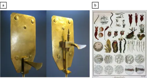
Being still hindered by the lens-making challenges, it was not until 1700 that significant magnification (270x) took place in the field of microscopy by the “Father of Microscopy and Microbiology”, Van Leeuwenhoek, who cleverly grinded and polished a small lens to be used in a simple microscope (i.e. a microscope with one lens) as seen in Figure 1.3 (a). He observed for the first time the “animalcules” (i.e. microorganisms) such as bacteria shown in Figure 1.3 (b). His simple microscope configuration was so powerful that it was still used till the middle of the 19th century. Although it was a remarkable progress, it wasn’t reliable enough; the microscope required mounting of the specimen on a needle-like holder situated just in front of the lens, where one’s eyes should be away from the lens by only a 1-cm distance.

(22)

5

Figure 1.3 The first observation of microorganisms. (a) Van Leeuwenhoek’s

microscope. (b) The “Animalcules” (or microorganisms) observed [13].

Hindered by the often-laborious handling of microscope, scientists needed to give one more look backward and try to tackle the instrumental challenges posed by the compound microscope setup with its multiple-lenses configuration. Around a century has passed until Joseph Lister in 1824 tackled the achromatic aberrations involving different focal planes for different wavelengths by designing the two-material type lens [14]. Subsequently, Schleiden and Schwam laid the foundation of the cell theory in 1838 and then came Ernst Abbe in the 1880s who optimized the resolving power of lenses through his grinding and sanding skills and developed the diffraction limit equation [15-17]. Afterwards, artefacts introduced by sample illumination such as glares and bulb filament images on the final image were overcome by August Köhler through his implementation of an auxiliary optical setup at the source side providing even illumination at sample surface with no constraints on the light intensity (i.e. Köhler Illumination) [18]. These breakthroughs constitute the cornerstone of old and modern versions of optical microscopy techniques.

Only by the end of the millennium, new light microscopy techniques started to “break” the diffraction barrier. These techniques were developed with the help of genetics which progressed to develop efficient ways in modifying the DNA reliably. This permitted any protein of interest to have fluorophores (i.e. fluorescent protein reporters) in its genetic construct which make the targeted protein fluorescent by itself, and thus easily tracked and imaged [19].

(23)

6

1.2.2 Electron Microscopy

Motivated by the diffraction limit in optical microscopy and the invention of the electromagnetic lens devised by Hans Busch, Enrst Ruska used the electrons as his source of illuminating radiation and built his own prototypes in 1930s. These prototypes exceeded the resolution achievable by the light microscopy at that time [20].

There are two main types of electron microscopes: the transmission electron microscope (TEM) and the scanning electron microscope (SEM). Their underlying principles are slightly different; in the case of TEM, the whole surface of the sample is subjected to electrons where the ones crossing the nm-scale-thick sample will diffract, carrying information about sample structure. These transmitted electrons are then magnified by the electromagnetic lens and get collected by appropriate detectors to generate diffraction patterns. In the case of SEM, not all regions on the sample surface are subjected to incoming electrons; an accelerated beam of electrons (i.e. primary electrons) is focused onto a single spot on the sample surface of typical diameter less than 10 nm and scanned in a “raster” manner. The interactions between the incoming electrons and surface atoms will lead to either elastically (backscattered) or inelastically (secondary) scattered electrons which are then collected and analyzed by the appropriate detectors (Figure 1.4). If backscattered electrons are collected and processed, the chemical composition of the sample surface can be determined. On the other hand, secondary electrons hold information about the sample topography [21].

(24)

7

TEM is concerned with revealing the interior (i.e. bulk) structure of a wide variety of biological samples like tissues, micro-organisms, cells, organelles and protein arrangements inside cell membranes. On the other hand, SEM deals with the sample surface, specifically its topography and chemical composition.

Despite their crucial roles in the world of microscopy today, TEM, for instance, requires sectioning of the bulk samples into very thin layers (not larger than 100 nm) so that the transmitted electrons can pass easily. SEM, on the other hand, typically needs several preparation steps like metal coating of insulating materials which is necessary for preventing the samples from being charged and damaged during imaging. There are other laborious procedures needed to prepare most biological samples, including stabilizing the sample through dehydration and fixation by certain chemicals. Moreover, almost all electron microscopes need a vacuum environment such that the electrons are not scattered by the molecules in the ambient atmosphere.

It was not, astonishingly, until 1986 that Ernst Ruska was awarded the Nobel Prize for building the first electron microscope, which was regarded as “an extension of the human eye” by the Royal Academy of Sciences. Still, he was awarded only half of it while the other half was awarded to two scientists who employed sharp probes to get close enough to sample surfaces to interact with them through forces and tunneling currents. This approach constitutes the main working principle of the Probe Microscopy family.

1.2.3 Probe Microscopy

It was always the dream of scientists to build microscopy techniques with atomic resolution facilitating the observation and even, the “manipulation” of single atoms. This was not achievable yet in the period of 1960’s to 1980’s either through light microscopy or electron microscopy techniques. Thus, instead of using sub-atomic particles (e.g. photons or electrons) to interact with the samples, researchers came up with the idea of using very sharp probes (i.e. extremely fine “needles”) to be employed in “feeling” (i.e. interacting with) the sample in the same way we use our finger tips to recognize what is around us, say in a dark room [23].

(25)

8

This way of thinking was first paved by the stylus profilometry technique which was previously used to estimate some surface properties like topographical roughness. Its working principle is very closely related to the phonograph (or turntable) in which a stylus (i.e. sharp probe) is being moved over a surface and thus suffers deflections/vibrations due to topographical features (i.e. valleys and hills). These vibrations modulate on the top of the stylus the distance between two fixed magnets and a sandwiched movable coil. This modulating distance will result in variations of the current generated in the coil, thus registering the information about the feature sizes while scanning [24].

Russell Young used the concept of the needle to build his microscope (topografiner) which generated the first image of a sample topography by probe mapping. He applied bias voltage between the tip (or the field emitter) and the conducting surface in order to generate field-emission current between them. The emitter-sample distance was on the order of nanometers and the applied voltage was somewhat high (tens of volts). The generated current was strongly dependent on the emitter-sample distance which was maintained by a servo loop mechanism. This feedback system served to keep this distance constant as much as possible while scanning by adjusting the voltage of the vertical piezo so that it moves to preserve a constant field-emission current. Still, the thermal instability and the mechanical vibrations that this system suffered from prevented the system to hold the current constant for multiple seconds. This prevented the method from detecting a much more delicate but very sensitive phenomenon that holds the key to unravel single atoms, namely: Quantum Tunneling [23, 25].

(26)

9

Figure 1.5 Early topography image taken by one of the first probe microscopes

(Topografiner) [26].

The quantum tunneling phenomenon involves electron transfer between two atoms which can occur when a (semi-)conducting, sharpened tip (sharpened to the extent that

at its foremost end, it will have only one or very few atoms) approaches a (semi-)conducting sample surface very closely. If a bias voltage is applied between tip

and sample, electron transfer can be induced over the vacuum barrier, despite the fact that the tip and sample are not “touching”. The tip-sample distance must be typically maintained below a nanometer to have quantum tunneling, and thereby measurable electric current. Because of its exponential distance dependence, tunneling was a very appropriate mechanism to be used as a microscopy technique aimed at high spatial

resolution (Figure 1.6) [27]. This gap-sensitive method required very precise (sub-nm-scale) mechanical control of the vertical position of the tip above the surface,

which can be regarded as the piece-de-resistance that Gerd Binnig and Heinrich Rohrer mastered and achieved in their scanning tunneling microscope (STM). Based on this invention, it they were awarded the Nobel Prize in 1986, together with Ernst Ruska for his TEM invention.

(27)

10

It took Binning and Rohrer less than a decade (1979-1986) to perfect the STM by solving diverse problems and to convince the scientific community that their microscope can take accurate images on the atomic scale based on the quantum tunneling effect. They tackled various issues such as reducing mechanical vibrations from the surroundings via mechanical suspension. In addition, they updated their setup with an acoustic hood to damp any acoustic noise. Initially, they faced problems in replicating their own scans. They argued that the reason was tip wear and thus they started working on sharpening the tip before each scan using high electric fields. Helped by their instrumental improvements, Binning and Rohrer provided images of different surfaces like Si of different crystallographic, as shown in Figure 1.7 (a). The final blow to doubts aroused in the scientific community was when Binning and Rohrer used their updated pocket-size STM to compare their atomic-scale images of graphite with its electronic structure which was easily calculated from theory, as seen in Figure 1.7 (b). This was when the STM “matured from an art to a technique” [23].

(28)

11

Figure 1.7 Scanning Tunneling Microscope (STM) images of (a) Si (111) and (b)

Graphite surfaces [23].

Although the STM made the scientists achieve their dream of “seeing” atoms, it could not be applied to all samples as it requires (semi-)conductivity for the effect of quantum tunneling to occur. This summoned and inspired the rise of a new microscopy technique that could image both conducting and non-conducting samples in air, liquid and vacuum environments, namely atomic force microscopy (AFM).

1.3 Atomic Force Microscopy

Atomic force microscopy (AFM), since its invention in 1986 [29], has overcome most of the limits associated with previous microscopes and also exceeded the “modest” dreams of just observing biomolecules and microorganisms at work. AFM has become much more revolutionary, in a sense it doesn’t only image with unpreceded spatial resolution but its nature of probing samples facilitated its ability to “interfere” widely with the processes being imaged and conduct measurements (i.e. spectroscopy) to quantify nanoscale properties associated with bio-macro-(nano-)molecules in their own native environment (i.e. liquid), with no considerable damage to the samples.

(29)

12

Combining the profilometry and the STM concepts, AFM utilizes an extremely sharp tip to laterally scan the sample surface under light contact thus generates topography images on different kinds of sample surfaces with sub-nm resolution. The sharp tip itself is attached to a micro-manufactured cantilever employed as a soft spring (with typical spring constant values below 1 N/m), which exhibits deflections in response to interaction forces arising between the tip and the sample during scanning. Using an optical setup, the minute deflections and hence, forces acting on the probe can be precisely measured (with sensitivity in the sub-nN regime). Feedback loops adopted from STM are employed to keep the tip-sample interaction forces at a constant value while scanning so that high-resolution images of sample topography are generated [30]. We will discuss the basic principles of AFM imaging together with force spectroscopy in Section 2.1.

AFM has made many cross-roads with so many fields like microbiology, immunology, biophysics, nanotechnology, and nanobiotechnology due to its very relaxed limitations on specimen choice, imaging environment, and easy sample preparation steps [31]. In that context, AFM has overcome the hardships in biology which the scanning tunneling microscope (STM) has suffered from [31], by combining the STM feedback capabilities with the profilometer advantages in a new scheme [29]. Once it was shown that the AFM can be used in imaging under fluidic environments [32-34], the doors were wide-open in front of many candidates from the biology world to be studied excessively [34-47]. For instance, AFM was exploited to investigate different kinds of bacteria [36, 43], filamentary structures [44], cell membranes [45], single proteins [37], as well as viruses [46] and genetic materials (Chromosomes and DNA) [39]. By functionalizing the AFM probe with nanoparticles and proteins, and approaching outer cellular membranes, even protein-cell interactions can be probed in-vivo [47].

Coming to the ability of force spectroscopy (i.e. probing the sample’s nanoscale mechanical properties), it was shown that AFM cannot only “feel” the sample as a nanoscale “finger” to image it, but it is also able to “press” on it to determine the mechanical properties of the sample. For instance, it can be used to probe the adhesive properties of samples contributing as main players in the mechanonanobiology field, giving us more insight into the structure-function relationships in adhesion [48-49]. Also, through the data (i.e. force-distance (FD) curves) collected by the AFM’s

(30)

13

“pressing” capability, differentiation between healthy and cancerous cells was possible [50]. Also, through tip “functionalization”, which is a major capability of AFM, force spectroscopy can detect and quantify mechanically the interaction between antibiotics and bacterial cell walls [51]. Functionalizing the tip with chemical groups (called chemical force spectroscopy) enables AFM to be chemically sensitive by mapping, for example, how strong the local receptors on the cell surfaces interact with specific chemicals on the tip, thus providing a deep look into the structure-function properties of the cells [52]. One of the most interesting applications of the tip functionalization is that it can quantify the intermolecular forces between the ligands and their receptors [53-55]. In the previous decade, new approaches that involve the simultaneous use of AFM with other imaging techniques have been invented. For instance, together with confocal microscopy (a type of light microscopy), AFM can probe the stiffening property of metastatic cancer cells before invasion [56]. Also, “correlative imaging” is possible while combining optical techniques with AFM to reveal physical links between different phenomena [57].

Due to the short time scales in which the dynamics of the biological processes change, fast AFMs (usually called high-speed AFMs, or simply HS-AFMs) have been developed in order to image (and in some cases, generate stiffness maps for) different biological samples like the famous Myosin V protein [58]. HS-AFMs also provide video-rate imaging of the dynamics of nanoscale structures such as various proteins associated with the cell membrane and antibodies [59-61].

Pressing our finger against a surface to see if it is hard or soft is a ubiquitous act that is developed as an efficient and crucial ability for our survival by making use of the materials around us. In the case of nanoscale materials, this ability can be mimicked by a “nano-finger” which is the AFM tip employed for indenting the samples under investigation and quantifying their stiffness. The pressing of the tip into the sample

(coined as a “nanoindentation” experiment) results in the acquisition of a Force-Piezo Displacement curve or shortly, a force-distance (FD) curve. Through the

processing of FD curves, employing theoretical contact models, certain mechanical properties of the sample can be extracted. As such, nanoindentation experiments have been performed in the past over a large variety of biological systems [34, 42, 44, 48, 56, 62].

(31)

14

One of the various biological samples that can be studied using AFM is amyloid nanofibers. It will be necessary and logically fundamental for the reader to be provided with a brief background about the specific biological system investigated in this thesis (i.e. bacterial functional amyloid nanofibers) before we delve into the experimental part in the next chapters and contemplate on the results obtained.

1.4 Amyloid Nanofibers

Amyloid aggregates present a class of thread-like and filamentous morphologies that can be accessed by several globular (particle-like) proteins of various amino acid sequences. Historically, they are known for their notorious association with a variety of chronic neurodegenerative diseases including the Alzheimer disease [63]. Amyloid formation is a polymerization process where soluble proteins can be transformed, through aggregation phenomena under certain (controlled or not) circumstances, to highly-ordered and/or misfolded hierarchical fibrillar structures in the extracellular environment [64].

Structures of amyloid proteins like Sup35, insulin, amyloid-beta peptide (Aβ), Tau, amylin, and prion protein were revealed [65-69]. There are some common characteristic properties that differentiate the amyloid fibers from other fibrils; the β-strands-rich core lies at the heart of the amyloids uniqueness. The molecular patterns taken by that core are arranged in a plenty of 3D shapes which seem to be part of an ever-growing collection. That diversity in molecular structures revealed by different imaging techniques seems to reflect the multiple amino acid sequences associated with the globular proteins. The amyloid formation seems to be guided via specific pathways reflecting its protein amino acid sequencing and thus organizing the β-strands in various forms inside the amyloid core perpendicular to the fiber axis. Those repeated cross β-strands are typically arranged in-register forming β-sheets, where the stacking arrangement differs from one type of amyloid to another, and thus enables plenty of different substructures to evolve. Consequently, these different atomic substructures together with the aggregation pattern seem to determine the functionality/toxicity of the respective amyloids [64, 70].

(32)

15

Figure 1.8 Biogenesis of amyloid nanofibers. (a) Amyloid formation at cell outer

membrane [71]. (b) Molecular model of amyloid fibril twisted along the direction into the page (i.e. the fibril axis) [72].

Although the functionality of the amyloids was discovered recently, it is believed that it can be dated back to the pre-biotic world as, astonishingly, the first functional protein structure [73]. The functional amyloids were found to exist in plenty of organisms such as fungi, bacteria, and even mammals. Moreover, they are known to be very useful towards unraveling the details of the “amyloidogenesis” process with implications for the growth and toxicity of pathological amyloids [73-74].

In this thesis, we will be investigating the functional amyloid nanofibers secreted by Escherichia coli (E. coli), which exhibit potential to be exploited as next generation dynamic biomaterials.

Curli fibers (or Curlins) are a compelling example of the functional amyloid nanofibers [75]. These bacterial fibrous proteins are extracellularly-secreted and classified as adhesins that aid E. coli bacteria to adhere to surfaces and assemble with other components, like cellulose, to form protective structures termed as biofilms. These biofilms offer a defensive shelter for large bacterial communities against harsh environmental conditions (e.g. extreme temperature, pressure, or pH) and also provide resistance against proteolysis, towards ensuring long-term survival. The curli fibers are regarded as the structural “spine” or “backbone” of these biofilm structures and play an

(33)

16

important role in determining overall mechanical properties. These curlins are synthesized by highly-controlled curli-specific genetic machinery which is encoded in the E. coli DNA by csg curli-responsible genes (i.e. csgDEFG and csgBA operons). The csg curli operons drive the expression of CsgD, CsgE, CsgF, and CsgG membrane secretory proteins which drives the extracellular secretion of the main precursors of the curli fibers: the minor subunit protein, CsgB, and the major subunit protein, CsgA. After these proteins (i.e. CsgA and CsgB) are secreted from the cell membranes, the polymerization (the fiber-assembly process) takes place on the outer-membrane of the cell [71, 76-77].

In this thesis, engineered genetic-mutants of E. coli are employed to extensively investigate functional amyloid nanofibers with different biochemical compositions via AFM imaging and nanoindentation experiments. The details of the experimental procedures and the obtained results are provided in the next chapters.

(34)

17

1.5 Outline

This thesis is divided into five separate chapters.

The current chapter (Chapter 1) presents an overview of the field of microscopy, specifically its history over the last few centuries. We briefly give an account on light microscopy, electron microscopy and the family of probe microscopy which the AFM belongs to. The STM (the predecessor of the AFM) is discussed in more detail by showing the improvements applied to it over years, as these improvements were directly transferred onto the AFM. AFM is introduced and several biological applications are listed. The chapter concludes by a brief intro to bacterial functional amyloid nanofibers. Chapter 2 contains the underlying working principles associated with AFM imaging and force spectroscopy. Also, it presents a discussion of AFM calibration steps involving extracting the photodiode sensitivity (𝑆) and the cantilever spring constant (𝑘𝑐𝑎𝑛𝑡) as well as the structural characterization of the tip apex via SEM. We conclude

by briefly touching on the preparation of amyloid nanofibers for AFM experiments. Chapter 3 includes an overview of practical procedures for AFM force spectroscopy. We discuss in detail the collection of the force-distance curves and their processing, which provides not only stiffness values associated with different amyloid nanofibers but also an estimation of the effect of the substrate on the measurements.

Chapter 4 presents the results of AFM experiments performed on 8 different amyloid samples in terms of morphological and mechanical properties (particularly, Young’s moduli). We also discuss the rational tuning of mechanical stiffness and the use of a qualitative method to compare the morphological properties of the samples. We discuss the results in the context of being a function of biochemical composition, and we utilize statistical analysis to evaluate significant changes in measured properties.

Chapter 5 finally provides a summary of the thesis and an outlook regarding future directions of research.

(35)

18

Chapter 2

2. Experimental Methods

2.1 Imaging and Force Spectroscopy

As briefly described in Section 1.2.3, the atomic force microscope (AFM) is able to generate images with unpreceded spatial resolution down to the sub-nm scale, together with the detection of tip-sample forces down to the piconewton regime. The main constituents underlying AFM operation are carried out by several instrumental parts designed and installed to work together in harmony. These involve: (i) the cantilever with the sharp tip, (ii) the laser source, (iii) the position-sensing photodiode detector, (iv) the electronic feedback system, and (v) the piezoelectric actuators (as partially depicted in Figure 2.1).

(36)

19

Figure 2.1 Simple schematic of AFM setup showing its basic operational principle [78].

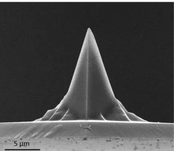
A micro-manufactured cantilever, with a nm-scale-diameter sharp tip (or simply probe) located at its end (as revealed under SEM in Figure 2.2), transduces the repulsive as well as attractive interaction forces emerging between its probe and the surface when they come into contact, into deflections. These forces originating from “touching” sample features with the probe, deflect the cantilever in upward and downward directions while moving on the sample surface. To detect these deflections, an optical method is used, as explained below.

A laser beam directed to the topside of the cantilever, reflects onto a four-quadrant position-sensing photodiode (or simply PD). The cantilever deflections are monitored by changes in the position of the laser spot on the PD (see Figure 2.1 and Figure 2.3). The PD comprises four segments as seen in Figure 2.3 (first panel on the left), where each segment (A, B, C, or D) has its own voltage intensity. At the beginning of the experiment, the AFM operator should align the laser spot to be at the center of the PD as seen in Figure 2.3 (second panel). At the set-point, the voltage differences between either the upper and the lower quadrants ((𝐴 + 𝐵) − (𝐶 + 𝐷)) or the left and the right quadrants ((𝐴 + 𝐶) − (𝐵 + 𝐷)) are tuned to be zero before starting any measurements, as seen in Figure 2.3 (second panel).

(37)

20

Figure 2.2 SEM image of the AFM cantilever tip used in this study.

During scanning, the “bumps and valleys” characterizing the surface topography of the sample cause the cantilever to deflect up or down in the vertical deflection, causing a change in the vertical position of the laser spot on the PD. For the sake of illustration, if a probe passed by a “bump” feature the cantilever would suffer an upward deflection that changes the optical beam path, whereby the laser spot on the PD will shift downwards as in Figure 2.3 (third panel). This downward shift can be precisely calculated from (𝐴 + 𝐵) − (𝐶 + 𝐷) as a voltage difference (the voltage signals are converted to deflection values, in nm, as described in Section 2.2.1). In the same way, lateral forces due to friction between the tip and the surface would cause the cantilever to undergo torsional twisting and the laser spot would move horizontally, as shown in Figure 2.3 (last panel). While this is very useful for nanotribology experiments, in this thesis we will not be focusing on this aspect and therefore, the twisting of the cantilever should not be discussed in much further detail.

(38)

21

Figure 2.3 Photodiode scheme and laser spot position as a result of cantilever deflection

[30].

After recording vertical voltage signals from the photodiode, they are sent to another part of the AFM setup, namely, the feedback controller, which takes the voltage signals from the photodiode and processes them to adjust the height of the cantilever over the sample surface in an appropriate way such that the deflection resets to a fixed set-point value during scanning. This height difference is recorded as the feature height at the point where the cantilever is deflected and topography maps are generated accordingly. For the sake of resetting the cantilever deflection to its set-point value, the piezoelectric z-scanner is actuated by the voltage signal from the feedback controller, and as such moves upwards/downwards to “relax” the cantilever and bring the deflection to its set-point value. To sum up, working together, the cantilever, the electronic feedback system and the piezoelectric scanner allow the probe to track effectively and accurately the topographical features on sample surface, as seen in Figure 2.4. Finally, by registering all movements of the piezoelectric scanner in the vertical z direction at all scanning points, 3D topographical images of complex sample surfaces can be generated as seen in Figure 2.5.

(39)

22

Figure 2.4 The AFM probe follows the sample topography in a smooth fashion as

mediated by cantilever deflections, the respective vertical movement of the piezoelectric scanner and the control signals from feedback system [30].

Figure 2.5 3D topography image of E. coli bacteria secreting networks of amyloid

nanofibers to the extracellular environment, obtained by AFM. The image size is 99 µm2 with a maximum height of ~200 nm [79].

(40)

23

When the tip never leaves the sample surface and is always in contact with the sample features while scanning, this AFM procedure (i.e. mode) is called contact mode. Although this is the most common AFM mode of operation, it is not the best fit for all samples, especially delicate ones that are weakly attached to their substrate. This issue is tackled by another AFM mode of operation called tapping mode.

Tapping mode involves excitation of the cantilever at its resonance frequency, causing oscillations. These oscillations are facilitated mainly by a piezoelectric element located at the cantilever holder driven by sinusoidal voltage signals. This mode not only cancels out any lateral “pushing” exerted by the AFM tip on weakly-attached specimens (as in contact mode), or preserve both the AFM probe and soft samples from wear and damage, but it also provides us with different channels of information about the sample. Precisely, the tip-sample interaction forces induce measurable changes in signals associated with cantilever oscillations such as: oscillation amplitude, frequency, and phase (sensitive to the sample composition). As in contact mode, any of these signals can be set to a reference value (i.e. “set-point”) such that any variations induced by scanning the sample surface can be sent to the feedback controller as the input signal. Alternatively, these signals can be recorded to make conclusions about the physical properties of the sample. The oscillation amplitude is used mostly as the feedback signal during tapping mode AFM, whereby the feedback loop attempts to keep it constant during scanning, allowing topographical measurements based on changes in the tip-sample distance, as in contact mode imaging. The underlying working principle of imaging via tapping mode is described briefly in Figure 2.6.

(41)

24

Figure 2.6 Basic principles of tapping mode AFM imaging [5].

“Feeling” the surface topography is not the only task that the AFM can perform. In particular, the capability of “pressing” into the surface is one of the main attractions that drove the scientists to use AFM extensively in studying several samples. Commonly termed as force spectroscopy, these experiment involve applying controlled deformations of the sample via the AFM tip by gradually “pressing” it into the surface, resulting in increasing interaction forces as reflected by larger cantilever deflections. The experiments typically result in the collection of force vs. distance plots (or simply, FD curves), as shown in Figure 2.7. Here, the tip-sample distance is controlled by the vertical displacement of the piezo scanner.

FD curves are classified into two types: approach and retractions curves. The approach curve in Figure 2.7 (starting with point A) comprises three main stages: At point A, the tip is away from sample surface and thus the cantilever is experiencing zero deflections (i.e. null forces), as expressed by the horizontal line. At B, while approaching the surface, attractive tip-sample forces pull in the AFM tip to the surface abruptly, as seen by the downward jump of the force to a minimum value, indicating downward deflections. Starting from B towards C, the cantilever is pressing (or indenting) into the sample via the tip apex and depending on the stiffness of sample surface, the rate of the

(42)

25

cantilever upward deflections (i.e. the slope of the line) will vary. Once the force reaches a pre-set maximum value, the retraction curve starts (i.e. the cantilever is pulled back from the surface). The D state resembles the retracting stage where the cantilever is moved up away from the surface. The attractive forces now delay the full detachment of AFM tip from the surface when compared to the pull-in stage during approach, as seen by the horizontal difference between the two dotted vertical lines. The force required to detach the tip from the sample surface (representing “adhesion”) is also larger than the pull-in force, as reflected by a deeper minimum. Nevertheless, this thesis is concerned with approach curves that are used to extract the “stiffness” of the samples.

Figure 2.7 Schematic diagram of an FD curve with different stages of probe-surface

interactions, via which various nanomechanical properties can be extracted [80].

The approach curves are characteristic to sample material in a way that collected curves from different materials most probably will exhibit differences in the associated slope values, indicating variations in nanoscale stiffness . For instance, the experimental FD curves shown in Figure 2.8 are acquired on genetically-different samples of amyloid nanofibers. The different slopes correspond to different mechanical stiffness; Highest slope corresponds to stiffest sample and lowest corresponds to softest sample (i.e. easily indented).

(43)

26

Figure 2.8 Representative FD curves extracted from force spectroscopy experiments

performed on three different amyloid nanofiber samples (to be described later). Different slopes indicate different mechanical stiffness.

As we previously mentioned in this section, cantilever deflections are recorded as voltage differences (Volt) on photodiode segments and to convert these into force values (in Newton) at the tip-sample interface, photodiode sensitivity and cantilever spring constant parameters should be precisely determined.

2.2 Calibration Procedures for AFM

2.2.1 Photodiode Sensitivity Parameter (𝑺)

The first step in AFM calibration procedures which is necessary to begin imaging and force spectroscopy measurements is the determination of the photodiode sensitivity parameter (𝑆). The sensitivity parameter is in the very origin of cantilever deflection calculations, which are traced by an optical setup. This optical setup involves a laser beam re-directed by the cantilever back onto a four-segment photodiode (see Section 2.1). The vertical movements of the laser spot on the photodiode are accompanied by voltage differences that reflect the cantilever’s upward and downward deflections. To transform these voltage variations on the photodiode (Δ𝑉𝑃𝐷, in Volts) to deflection

values (𝑑, in nm), the 𝑆 parameter (of unit: nm/V) is needed. In that regard, the three values can be related to each other through the following equation:

(44)

27

𝑑 (𝑛𝑚) = 𝑆 Δ𝑉_𝑃𝐷 (2.1) In order to extract the 𝑆 parameter experimentally, we perform force spectroscopy measurement (as described in Section 2.1) by acquiring FD curves on the mica subtsrate surface which is regarded to be “infinitely hard”, and thus, exhibiting no indentation. As such, the entire downward movement of the z-piezo scanner (the piezo displacement, 𝑍) is reflected in the cantilever deflection 𝑑 (i.e. 𝑑 = 𝑍). Thus, the sensitivity parameter 𝑆 can be extracted as the inverse of the slope belonging to each FD curve obtained on a mica surface (like the experimental curves shown in Figure 2.9).

To be more confident and precise in calculating the 𝑆 parameter value, we collect several FD curves (~10) on the mica substrate per force spectroscopy experiment (as seen in Figure 2.9). We then take the largest 𝑆 value (which is associated with the lowest indentation that resembles most closely the ideal condition of an infinitely hard surface) for carrying out deflection calculations. In our experiments, all extracted 𝑆 values are centered around ~300 nm/V. This means when cantilever deflection reaches 300 nm, the laser optical path shifts the laser spot position on the PD such that a 1 V voltage difference is measured across it.

Figure 2.9 Photodiode sensitivity calibration. Several FD curves are taken on mica

(45)

28

Because imaging more than one sample or imaging a single sample for a long time (~hours) can influence the 𝑺 values and cause changes, we perform the related calibration step twice per sample to calculate 𝑺_{𝒃𝒆𝒇𝒐𝒓𝒆}, taken before the sample, and 𝑺_{𝒂𝒇𝒕𝒆𝒓}, taken after the sample. We choose only one of the two values to convert voltages to deflections per sample. This choice depends on when most of the nanoindentation experiments were carried out on the sample. If they were conducted towards the beginning of the measurements, we choose 𝑺_{𝒃𝒆𝒇𝒐𝒓𝒆}, otherwise we choose 𝑺_{𝒂𝒇𝒕𝒆𝒓} as the final sensitivity parameter (𝑺𝒇𝒊𝒏𝒂𝒍). At the end, the 𝑺𝒇𝒊𝒏𝒂𝒍 value is used to process the

curves acquired from force spectroscopy experiments on a given sample and convert them from voltage vs. piezo displacement curves to deflection vs. piezo displacement curves. We list in the table below (Table 2.1) all the 𝑺𝒃𝒆𝒇𝒐𝒓𝒆, 𝑺𝒂𝒇𝒕𝒆𝒓, and 𝑺𝒇𝒊𝒏𝒂𝒍 values

that we have recorded for each sample of the amyloid nanofibers.

Table 2.1 Cantilever sensitivity parameters for all amyloid nanofibers.

𝐒𝐚𝐦𝐩𝐥𝐞𝐬 𝑺_{𝒃𝒆𝒇𝒐𝒓𝒆} (nm/V) 𝑺_{𝒂𝒇𝒕𝒆𝒓}(nm/V) 𝑺𝒄𝒉𝒐𝒔𝒆𝒏(nm/V) CsgA 336.7 339.1 336.7 CsgB 339.1 334 334 CsgAB 334 344.6 334 CsgAM 330.7 310.1 310.1 CsgBM 310.1 339.6 310.1 CsgAM-BM 293.6 293.2 293.2 CsgAM-B 296.9 298.5 296.9 CsgA-BM 298.5 296.9 296.9

2.2.2 Spring Constant of the Cantilever (𝒌_{𝒄𝒂𝒏𝒕})

High-resolution AFM imaging in contact mode and force spectroscopy via AFM requires the precise measurement of the normal forces acting on the AFM tip. In contact mode, the AFM instrument measures the cantilever deflection in the vertical direction (i.e. the z-direction) at each pixel of the image taken on the surface and then using the implemented electronic feedback mechanism in the AFM setup, the piezoelectric z-scanner (responsible for moving the cantilever base up and down) will adjust the height of the cantilever to keep the load applied by the tip to the sample surface (and thus the cantilever deflection) constant while imaging. This normal load (i.e. force) is calculated simply from Hooke’s law, 𝐹 = 𝑘_{𝑐𝑎𝑛𝑡}∗ 𝑑, where 𝑑 is the cantilever

(46)

29

deflection, and 𝑘_{𝑐𝑎𝑛𝑡} is the cantilever spring constant which is a characteristic parameter for each cantilever.

Many methods in literature have been proposed to determine with precision the normal spring constant of AFM cantilevers but the method developed by Sader et al. is the most widely used by scientists due to its plainness, reliability, and robustness [81]. As such, it was used in this thesis to calibrate the single cantilever, used in all experiments, by finding its spring constant value (𝑘_{𝑐𝑎𝑛𝑡}).

This method requires the knowledge of the resonance frequency of the cantilever, its geometrical dimensions, its mass and the density of the material it is made of. The reflective film of Aluminum (Al) used to direct effectively the laser spot towards the photodiode (PD) can affect the value of the cantilever spring constant and that is why this method accounts for it.

For a rectangular cantilever, the uncoated normal spring constant (𝑘_{𝑢𝑛𝑐𝑜𝑎𝑡𝑒𝑑}) can be obtained as:

𝑘𝑢𝑛𝑐𝑜𝑎𝑡𝑒𝑑 = 𝑀𝑒 𝑚 𝜔𝑢𝑛𝑐𝑜𝑎𝑡𝑒𝑑 2 (2.2)

where 𝑀_𝑒 is the normalized effective mass which relies on the aspect ratio of the cantilever (i.e. length/width); 𝑚 is the uncoated cantilever mass; 𝜔𝑢𝑛𝑐𝑜𝑎𝑡𝑒𝑑 is the

angular resonance frequency of the “uncoated” cantilever in vacuum (2% of its measured value in air is added to account for the difference between the air-damped and the vacuum environments [81]). These parameters are as follows: 𝑀𝑒 is taken as 0.2427

based on the length-to-width ratio (𝑙/𝑏); 𝑚 is simply the product of the cantilever material density (that of Si) and its volume (provided by the manufacturer datasheet in terms of the cantilever dimensions); finally, 𝜔_{𝑢𝑛𝑐𝑜𝑎𝑡𝑒𝑑} is known thanks to another equation that relates the angular frequency of the coated cantilever (𝜔𝑐𝑜𝑎𝑡𝑒𝑑) which is

typically measured by the AFM instrument software, to that of the uncoated one (𝜔_{𝑢𝑛𝑐𝑜𝑎𝑡𝑒𝑑}) which is needed above for the 𝑘_{𝑐𝑎𝑛𝑡} calculation. This equation is [81]:

𝜔𝑢𝑛𝑐𝑜𝑎𝑡𝑒𝑑

𝜔𝑐𝑜𝑎𝑡𝑒𝑑 = √1 +

𝜌𝐴𝑙 ℎ𝐴𝑙

𝜌𝐶𝑎𝑛𝑡 ℎ𝐶𝑎𝑛𝑡 (2.3)

where 𝜌_{𝐶𝑎𝑛𝑡} and ℎ_{𝐶𝑎𝑛𝑡} are the cantilever density and thickness, respectively, while 𝜌_𝐴𝑙 and ℎ_𝐴𝑙 are their counterparts for the Al film coated on the back of the cantilever.

(47)

30

Finally, the spring constant of the coated cantilever (𝑘_{𝑐𝑜𝑎𝑡𝑒𝑑}) can be related to that of the uncoated cantilever (𝑘𝑢𝑛𝑐𝑜𝑎𝑡𝑒𝑑) by the following equation [81]:

𝑘_{𝑐𝑜𝑎𝑡𝑒𝑑} = 𝑘_{𝑢𝑛𝑐𝑜𝑎𝑡𝑒𝑑}(ℎ𝐴𝑙+ℎ𝑐𝑎𝑛𝑡

ℎ𝑐𝑎𝑛𝑡 )

3 _𝐸

𝑒

𝐸𝑐𝑎𝑛𝑡 (2.4)

where 𝐸_𝑒 represents the effective Young’s modulus that accounts for both the elastic modulus of the cantilever material (Si) and that of the coating film (Al) which can be expressed by the equation below [81]:

𝐸_𝑒 =𝐸𝑐𝑎𝑛𝑡ℎ𝑐𝑎𝑛𝑡+𝐸𝐴𝑙ℎ𝐴𝑙

ℎ𝑐𝑎𝑛𝑡+ℎ𝐴𝑙 (2.5)

Within the context of this method, the single AFM cantilever used in our experiments turned out to have an overall spring constant value (𝑘_{𝑐𝑜𝑎𝑡𝑒𝑑}, or generally 𝑘_{𝑐𝑎𝑛𝑡}) of 0.20 N/m based on the data provided in Table 2.2, which lists the dimensional and material properties of the cantilever and its Al coating.

Table 2.2 Physical properties of the cantilever and its Al coating used in determining

the spring constant of the cantilever.

𝒍 (µm) 450 𝝎𝒖𝒏𝒄𝒐𝒂𝒕𝒆𝒅 (rad/s) 2** 𝒇𝒖𝒏𝒄𝒐𝒂𝒕𝒆𝒅

𝒃 (µm) 50 𝒇𝒖𝒏𝒄𝒐𝒂𝒕𝒆𝒅 (Hz) 13,688

𝒉_{𝑪𝒂𝒏𝒕} (µm) 2 𝒉_𝑨𝒍 (nm) 30

𝑬𝒄𝒂𝒏𝒕 (GPa) 130 𝑬𝑨𝒍 (GPa) 70

𝝆_{𝑪𝒂𝒏𝒕} (g/cm3) 2330 𝝆_𝑨𝒍 (g/cm3) 2700

2.3 Tip Apex Characterization with SEM

A single probe (NanoSensors PPP-CONTR) has been utilized for all AFM measurements discussed in this thesis. The characterization of the tip apex by finding an estimate of its radius (𝑅) is necessary for extracting accurate Young’s modulus values from force spectroscopy experiments.

𝑅 can be estimated using scanning electron microscopy (SEM) imaging discussed previously in Section 1.1.2. Briefly, secondary electrons are used to obtain images of AFM tip apices as in Figure 2.10, such that extracting the 𝑅 value is straightforward.