Low-temperature thermodynamics of finite and discrete quartic quantum oscillator in one dimension

(1)

L O V V ^ ™

O F

# I N I №

i : “

-r

:,- ^ s u B M r i^ i0 T O 'T №

-

a

ND THE INSTlT!:]TE’0r;:ENGINEERiNG:3^N

;■;:·_, ^ /:'■ ■■ V - : : : : ' d E - i R i : K i i ^ U N i f E R S i t Y ; . ;'a '

IN PARTfttltJi;>FIlAMENTp THE REpumEMEN'TS^:

:,■ ' ^::· -FOR THE'HEGREE

o f

’'

• ; -MASTER OF SCIENCE .

Q c W 3 S S S S / S S B

B y

A fif SlD D IK i

September 1999

(2)

LOW-TEMPERATURE THERMODYNAMICS OF

FINITE AND DISCRETE QUARTIC QUANTUM

OSCILLATOR IN ONE DIMENSION

A DISSERTATION

SUBMITTED TO THE DEPARTMENT OF PHYSICS AND THE INSTITUTE OF ENGINEERING AND SCIENCES

OF BILKENT UNIVERSITY

IN PARTIAL FULFILLMENT OF THE REQUIREMENTS FOR THE DEGREE OF

MASTER OF SCIENCE

By

A fif Siddiki

September 1999

(3)

«ς ει , es s 5£ И-Я 2 ' Н у ''" Г)

(4)

I certify that I have read this thesis and that in my opinion it is fully adequate, in scope and in quality, as a dissertation for the degree of Master of Science.

Asst. Prof. T u^ul Plakioglu (Supervisor) I certify that I have read this thesis and that in my opinion it is fully adequate, in scope and in quality, as a dissertation for the degree of Master of Science.

I certify that I have read this thesis and that in my opinion it is fully adequate, in scope and in quality, as a dissertation for the degree c ’’ Mac:-er of Science.

Approved for the Institute of Engineering and Science:

Prof. Mehmet Bcira;^

(5)

ABSTRACT

LOW-TEMPERATURE THERMODYNAMICS OF FINITE

AND DISCRETE QUARTIC QUANTUM OSCILLATOR IN

ONE DIMENSION

Afif Siddiki

M.S. in Physics

Supervisor: Assistant Prof. Tuğrul Haldoğlu

September 1999

I.' this work we examined a quartic Hamiltonian using two different ap proaches. We first introduced a mean-field Gaussian approximation in order to handle this Hamiltonian analytically and observed that this approximation is insufficient for all coupling strengths. Hence we applied second and third order non-degenerate time-independent perturbation and obtained third or- ■ ler correcHo

::3

to the four-body co’-i.elation

7

..

In the second part we introduced a new representation for the many-body wave functions and implemented this representation to our numerical tech niques. By the use of this technique we examined some thermodynamical properties of a discrete-finite interacting one-dimensional system for differ ent interaction functions. We introduced some possible criteria in order to understand the thermodynamical properties for such a system. Finally with in the light of these considerations we observed Bose-Einstein condensation like behavior for a particular coupling.

K e y w o r d s : Anharmonicity, high temperature superconductors, mean- field a.pproximation. discrete-finite systems, Bose-Einstein condensation.

(6)

ÖZET

AYRIK VE SONLU BİR BOYUTLU DÖRDÜNCÜL

KUANTUM SALINICISININ DÜŞÜK SICAKLIKTAKİ

TERMODİNAMIİK ÖZELLİKLERİ

Afif Sıddıki

Fizik Yüksek Lisans

Tez Yöneticisi: Yard. Doç. Tuğrul Hakioğlu

Eylül 1999

Bu çalışmada dördüncü dereceden bir Hamiitonyeni iki değişik yöntem ile inceledik. İlk önce Gaussiyen bir ortalama-alan yaklaşıklığı kullanarak bu Hamiitonyeni analitik olarak ele aldık, ve bu yaklaşıklığın her çiftlenim büyüklüğü için geçersiz olduuğunu gözlemledik. Bu sebepten ötürü ikinci ve üçüncü dereceden yoz olmayan, zamandan bağımsız perturbasyon kuramını kullanarak dört-parçacık korrejasyorıla”’ ’ '·' '" - " ’-u"" ^¡ore-f^den eld-: ettik.

ikinci kısımda çok-parçacık dalga fonksiyonlarının yeni bir gösterimini sunduk ve bu gösterimi nümerik yöntemimizde uyguladık. Bu yöntemi kul lanarak sonlu-ayrık ve etkileşimli bir boyutlu bir sistemin bazı termodinamik özelliklerini değişik etkileşim fonksiyonları için elde ettik. Bu tür bir sis temin termodinamik özelliklerini anlamak için olası yeni kriterler önerdik. Son olarak bu yöntemlerin ışığı altında belirli bir etkileşim fonksiyonu için Bose-Einstein yoğuşması benzeri bir davranış gözlemledik.

A n a h ta r K e lim e le r : Anha.rmoniklik, yüksek sıcaklık süperiletkenliği, ortalama-alan yaklaşıklığı, aynk-sonlu sistemler, Bose-Einstein yoğuşması.

(7)

ACKNOWLEDGMENT

” Ya§am.ak bir ağaç gibi tek ve hür ve bir orman gibi kardecesine,

biL hasret bizim...’'

I am indebted to my thesis supervisor Assist. Pi'of. Tuğrul Hakioğlu for many valuable criticisms and suggestions not only for this thesis also for his advises to be a ’’good” physicist. I am thankful for his patience and encouragement.

■ I should thank to my teachers who brought me here to complete this study. In particular to Prof. Ayşe. Erzan and Prof. Enver P. Nakhmedov from Istanbul Technical University and especially to Assoc. Prof. Bilal Tanatar from our physics department, for his scientific assistance and encouragement since the beginning of my graduate study.

I would like to express my deep gratitude to my ’’ Bilader” 1. Bülent Özge for his sensitivity and encouragement. In particular for hie moral and financial assistance which I could not get from elsewhere.

My special thank goes to Ibrahim ’’ Hocam” and Mr. Ceyhan, who man aged make time to share this prison life together and for their advises which I would keep in mind for a life time.

My office-mate, Sencer Taneri, I would like to thank for his patience and friendship. Especially for having coffee with cigarette together while our office was up-side-down.

As I look back to see who all made this study possible, my thoughts first run to my mother, who is also my friend, my advisor and my loneliness.

(8)

I would like to extend my indebtedness to my ” Aba” . 1 had the privilege to consult him in any personal troubles, I will keep my promise and keep on struggling for my principles. Then comes my little sister, Feride, whom I learned how to study persistently with peace of mind of-course with her delicious mid-night cakes and discussions about the relation between physics and archaeology. My sweet angel, I really do not know how to express my ap preciation and admiration for your patience, encouragement and confidence, beyond these I am thankful for her intension for being a ’’ dost” of mine.

(9)

List of Figures

3.1 The two-body correlations as a function of coupling strength A. 19 3.2 The four-body correlations as a function of coupling strength A. 20 3.3 The dependence of the 2"·^ and the 3’’*^ order corrections to the

four-body correlations and the four-body cumulant with the order corrections as a function of coupling strength A. 25

4.1 One-dimensional lattice in configuration space... 28 4.2 One-dimensional reciprocal lattice in momentum space... 28 4.3 One-dimensional reciprocal lattice with cyclic boundaries. Ar

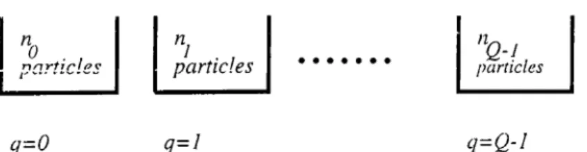
rows sketch the Umklapp processes... 29 4.4 A schematic representation of our proposition, tiq particles

situated at slot c =

0

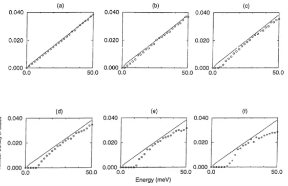
etc.., 30

5.1 The density of states for (a) t; — 2 (b) ?/ = 1 . 5 ...37 5.2 The number density of states for constant type interaction (a)

A = 0.1 (b) A = 0.25 (c) A = 0.5 (d) A = 0.75 (e) A =

1

(f) A = 1 .5 ... 39 5.3 The number density of states for sine type interaction (a) A =

0.1, (b) A = 0.5, (c) A =

1

... 40 5.4 The number density of states for cosine type interaction (d)

A =

0

0.1

(b) A =

0

.

5

(c )A = l ...·... 47 5.13 The specific heat for sine type interaction (a) A = 0.1 (b)

A = 0.5 (c) A = 1...47 5.14 The specific heat for constant type interaction (a) A = 0.1 (b)

A = 0.5 (c) A = 1...48 5.15 Chemical potentials for (a) cosine (b) sine (c) constant type

of interaction with fixed = 50...49

(13)

Chapter 1 Introduction

From the beginning of century, with the improvement in the exper imental techniques, low-temperature behavior of materials became an inter esting field in experimental physics. In particular the experimental discovery of the first superfiuid material ('*He) in 1908 and superconductivity of mer cury by Kamerlingh Onnes in 1911 [1], has fascinated physicists.

However, the theoritical background has been constructed almost 15 years later within the realization of Bose-Einstein condensation (BEG) for non-interacting bosons in three-dimension[2][3]. It was first proposed by Eondon[4] that BEG can be a microscopic explanation for the superfludity phenomena. Superiluclity and superconductivity nas been generally associ ated with a specific type of order which London[5] called long-range order of the average momentum.. The earliest mathematical characterization of this order was given by Ginzburg and Landau[

6

] for superconductivity and by Penrose[7] for superfludity.

In 1967 Hohenberg[

8

] has shown that the long-range order is not consis tent with exact sum rules in one and two dimensions for liquids in homoge neous thermodynamic equilibrium. The question of BEG in inhomogeneous liquids was handled by Widom[9]. He concluded that inhomogeneities in the ideal Bose liquid can be accompanied by BEG. In his work the dynamical processes is left completely unresolved. Since then several authors exhib ited BEG in one di.mension for non-interacting Bose gcis for гш attractive i-im purity[

10

] and for power-law potentials[ll], [

12

] using different methods.

(14)

Recently ВЕС in a one-dimensional interacting system due to power-law trap ping potentials has been examined[13] by using mean-field Gross-Pitaevski equation within the semi-classical two-fluid model.

The well established wisdom is that, non-interacting systems in dimen sions less than three under the presence of external power-law potential more confining than a parabolic one exhibit ВЕС. For two-dimensional sys tems any power-law potential seems to raise to the critical temperature of ВЕС. The presence of ВЕС for dynamically interacting system hcis only be ing lately taking attention. A mean-field Gaussian approximation to the number conserving quartic interaction hcis been recently advocated from the group theory point of view[14]. Nozieres[15] has argued that the influence of the (dynamical) exchange interaction favors that the particles are cumulated non-uniformly in the momentum space. This agreement is based on a com binatoric analysis and is independent from the relative energy differences of the energy eigenstates. He has argued also that this implies a genuine ВЕС driven by exchange correlations. One of our basic motivation for studying quartic interaction is based on this agreement.

On the other hand the progress in producing superconducting materials with transition temperatures higher than about

20

°/v stagnated until the discovery of the high temperature superconductivity (HTS) of the layered copper-oxide compounds by Bednorz and Müller et а/.[

1

б]. Many differ ent theoritical explanations has been proposed, but by now none of these could be either proved or rejected on firm grounds. Among these proposals, conventional electron-phonon mechanism, is stib under disrussion An other motivaton for this study is based on the recent experiments for the oxide superconductors in which the strong low-temperature anomalies of certain vibrational modes [17]-[22] has been observed. This is a reflection of the strong coupling of the electronic and the lattice degrees of freedom[23].

Information about the static as well as dynamic state of the crystal comes from neutron scattering and optical (Raman,infrared) experiments. Phonon spectrum was of significance in developing the microscopic theory of pairing in conventional superconductors[24].

The phonon spectrum is obtained by using the fact that electron-phonon interaction leads to the renormalization of ionic frequencies cuqj, ( q, is a wave

(15)

vector,

5

is a polarization index) considering the relation given by

n L = ^ 2u^sRe^^s{n =

0

^,). (1.1) Here ilqs is the renormalized phonon frequency, Sqs is the phonon polariza tion. The real part of the pohiiization gives the phonon shift dcUqg and the imaginary part gives rise to finite lifetime l /

7

qs which is directly related to the Eliashberg function as

1

E

- a ,.)

TrhN{0) ^ Hqs (1.2)

where A^(

0

) is the density of electronic states on the Fermi surface.

The phonon density of states (PDOS) F {oj) is obtained from the inelastic

neutron scattering data. Thus an estimate for electron-phonon coupling can be obtained from the phonon frequency shift «^Wq^^ due to the resonance Raman scattering experiments .

The phonon dispersion curves throughout the Brillouin zone for typi cal high temperature superconducting crystals such as N dCu0 4, La2C u0 4 and Y B ü2Cuz0 7-x [25][26] have been obtained after synthesizing sufficiently

large single crystals .

Early investigations of the inelastic neutron scattering measurements on polycrystalline Y B ü2Cuz0 7-x revealed strong changes in the phonon spec

trum in transition from insulating to metallic state as the oxygen concentra- was· varied from non-superconducting x —

1

to superronducticg firhy- doped a: = 0 limit[27, 28]. Changes are observed in the low energy (i.e. 15 — 20meV) part of the phonon spectrum due to the doping of the 01 sites which affects the oxygen valency and the average number of C u l-01 and Cul- 0 4 bonds. However an essential increase in the phonon density of states is observed in the 40 — 80 m eV range corresponding to the vibrations of 02, 03 and Cu2 in the planes. Parallel to these changes, significant softening is ob served in the in-plane force constants. The increase in the PDOS in the high energy (> 40meP) regime can not be explained by structural changes alone. Thus authors[29] concluded that this effect is due to strong electron-phonon interactions. Similar experiments has been done by several authors[30][31] and it has been shown that, from the Raman active phonon at 333cm~^, the phonon softening in the superconducting state vanishes if superconductivity is destroyed by magnetic field just below T^, at a constant temperature[32].

(16)

This, together with the fact that four of the five Raman iines do not show any softening beiow Tc, strongiy suggests that the phonon softening beiow Tc reflect directly the coupling between these particular phonon with electronic states which take part in the formation of Cooper pairs.

We make the argument, also bcised on experiments done by Arai et

a/., [33], where a marked enhcincement of the structure factor is observed as the temperature is varied across Tc at the Brillouin zone boundary, that, the anhiirmonicity is unavoidable when a phonon frequency is abnormally softened, resulting in large amplitude vibrations of the corresponding mode. Large amplitude vibrations broaden the real space phonon wave function. Conversely, the phonon frequency softening can be observed as a result of low temperature anharmonicity[34j.

In summary, the observations of strong electron-phonon coupling and low temperature anharmonic effects cire likely to be the major source of the phonon anomalies observed in the high temperature superconductors. Thus we will examine a model anharmonic Hamiltonian in order to understand the exchange energy contributions due to correlations for a phonon subsystem. These observations of phonon anharmonicity in HTS and the recent intense studies of EEC in low-dimensions together motivated us to study the low- temperature thermodynamics of a quartic interaction in one dimension. Our approch to this problem is two-fold: first we handled the problem using an analytical approach which is based on a mean-field Gaussian approximation and observed that this approach is insufficient then, by the use of a new numerical method we examined some thermodynamic pronertR·’ . n hn’ ''e- discrete quartic quantum oscillator. The pursue which will be followed in this thesis is that; the notation and preliminaries will be introduced briefly, in the second chapter, beginning from the simple harmonic oscillator Hilbert space and Heisenberg algebra. Then these results will be extended to many-body systems in a qualitative manner. Third chapter will deal with the derivation of our model Hamiltonian, then we will introduce our Gaussian approxima tion, which is based on the correlation generating function. Furthermore, we devise a microscopic low temperature anharmonic model for the bare phonon subsystem and explicitly present its self-consistent low temperature solution. At the end of this chapter we will study momentum independent case and check the accuracy of our formalism.

(17)

A aumerical technique will be developed in chapter 4 in order to diago

nalize our model licimiltonian. VVe will introduce a new isomorphic repre sentation for the rnany-body wave function and discuss the implementation of this representation lor numerical purposes, in the last part of this chcipter some thermodynamic properties will be considered as a brief summary.

in chapter five which we suggested a new criterion for ВЕС as applied to discrete, finite and one-dimensional interacting system. VVe will apply this criterion to our one-dimensional anharmonic model where the interaction is the dynamical quartic exchange interaction. The idiermodynamic properties of this model system will be discussed paying specific attention to the like presence of ВЕС.

The results which has been obtained from the analytical approach can be extended to higher dimensions and also not just for bare phonon subsys tems also for electron-phonon systems using higher order corrections, thus the connection between phonon anomalies and superconductivity can be studied. Furthermore using the numerical technique electron-phonon systems can be handled for one or two-dimensional Hubbard-Holstein models. The like pres ence of ВЕС which is in principle accompanied with a phcvse transition can be justified by the experiments manifested in the ‘’ quantum-wires” , where we have finitely many degrees of freedom.

(18)

Chapter 2 Preliminaries

2.1 Introduction

VVe shall start our discussion by a well-known model, namely simple harmonic oscillator (SHO). A standai'd way of starting the discussion for a quantum oscillator is to introduce Hamiltonian which is given by

Ù

2-^2

H = --- h - m u X

2m

2

(

2

.

1

)

where p is the momentum operator of the quantum panicle with mass m and

X is the position operator of the particle oscillating with frequency u near a

stable equilibrium position. The operators obey the canonical commutation rules.

,P = ih

(2 2)

First part of eqn.(2.1) is the kinetic and second part is the potential energy terms. This is a quantum particle whose state vector obeys the Schrödinger equation

in—

(19)

2.2 The Diagonal Representation

in The Energy Eigen Basis

Now we concentrate ourselves on the energy basis leH) whose energy eigen value is e„. Let us write time-independent Schrödinger equation such that

H n -- - n

where n is a positive integer.

The energy basis e „ ) satisfies orthogonality

i^£n' -- ^n',n and completeness

E k « = 1.

Sn

We now introduce a new operator

“ = (v fJ p

and it’s Hermitian conjugate

1

2h ^ ^2mujh'

Then one can show that, a representation is permitted such that,

axid £«) = n" £n+i) (2.4) (2,5) (

2

.

6

) (2.7)

(2.8)

(2.9)

(

2

.

By the help of these definitions above the Hamiltonian (

2

.

4

) can be rep resented as

H = ku{â^à +

_(2.13)

The operators a\ a and N then have the Heisenberg algebra satisfying [iV, à] = —à , [yV, cr] =tl _ At

and

a, a

1 = 1

(2.14)

(2.15)

A much detailed discussion can be found in any standard quantum mechanics text book. This level of introduction will be sufficient for the completeness of the following chapters. One can easily generalize this one-dimensional harmonic oscillator formalism to represent many-body systems in terms of one-body harmonic oscillator basis. In the later chapters of this thesis we will be interested in many-body interacting systems exchanging energy and momentum via a quadratic interaction in which we will meet some of the notation as well as the concepts of this many-body extension.

2.3 Many-Body Hilbert Space

In the formulation of the one-dimensional quantum harmonic oscillator en ergy is described by the quantum mechanical operator N. The eigenvalue

n implies that there are n particles each having energy quantum hu> in the

eigenstate |e„^ where = (n

-|-The many-body approach is based on an extension of one-body to more than one modes (in our case this applies to more than one momentum eigen state) of a number of non-interacting harmonic oscillators each describing a single momentum mode k. The many-body wave function of such a sys tem of non-interacting harmonic oscillators should also be indexed by these good quantum numbers k. A naturally simple choice of a such many-body wave functions is a trivial extension of one-body wave functions in the direct product form

(21)

for a many-body system for K independent components. It is clear that this basis satisfy orthogonality

{n^Tl2 · · · ^

1^2

· · · ^‘KI ,rij ^n

2 ,«2

‘ ' ' cind completeness ^ \n1n2 .. .riK){^:)<7гır¿2 ...riK

=

1

(2.17) (2.18) n\ Tl2’-’nj^

Since our approach is based on extending a single mode bosonic case to many mode non-interacting bosons we have the extension of the eqn.(

2

.

1

) ¿is

a/:, a\i — 6k,k

and

[di, df] = [«l, “I j

=0

Chapter 3 The Analytical Approach

3.1 Introduction

In principle it is well known that lattice dynamical quantum fluctuations due to the anharmonicity becomes important at sufficiently low temperatures. This is mainly because of the fact that harmonic contribution to ions can be dominated by low temperature quantum fluctuations in energy and mo mentum by sufficiently high anharmonic coupling in otherwise independent modes. The importance of anharmonicity at high temperatures beccxme an even more interesting problem paralleling the developments in understanding the high temperature superconductivity. One of the techniques that has been developed is the Quasi-anharmonic approximation [37]. This method maps a weak anharmonic model onto an equivalent harmonic one which amounts to renormalizing the model parameters by thermal effects.

(23)

3.2 The Model Hamiltonian

3.2.1 Derivation

We shall start with the usual Taylor expansion for the crystal potential energy

V for small displacements around its equilibrium state. All calculations will

be done in one-dimension and for spinless particles.

Let a unit cell of the crystal be situated at position vector x and a is the unit cell parameter. One can define the displacement vector of the atom situated at xa to be u (x a ). The expansion is for small displacements u (x a ) around (x a ) as (for the short-hand notation xa will be fixed to r)

dV V = Vo+ dUa U

1 V

Ua{r)ui}{r')

d^V

^ 0-,^^c<{r)dup{r')du^{r") Ua{r)up{r')u^{r")

1

+ m Pt

d‘^V

Ua{r)ui3{r')u^{r'')Ur^{r'") .

(3.1)

For the equilibrium state to be a minimum the condition is that

dv

dUa{r) _lU

=

0 (3.2)

After fixing the constant term Vo to zero, one can write the crystal Hamilto nian up to fourth order in potential eneigy as

H = T + V2 + V s + V4

=

+

E

® « i ( r , r 'K ( r ) u ,( r ') r {r}ap '^c>p'y(r,r\r'yLjr)ui3(r')Uy{r'') {r}ap^ + ^

X!

S„/

3

.^„(r,r',r",r"')W a(i’)'ii/

3

(^')''^

7

(^")«r,(r’ ) {r}ap^V

(.3.3)

11

(24)

where p(r) is the momentum of the atom located at r. <I>, ^ and E are elastic tensors oi the second, third and the fourth rank respectively. If we assume Born-von Karman cyclic boundary conditions we may introduce a new set of second quantized coordinates (a normal set) by defining

h

¿mcur

■<(6)e‘’*(o, + al,)

where q denotes the direction of propagation of phonon modes, e,j{b) is the polarization vector in the longitudinal or transverse direction cind tu, is the corresponding phonon frequency dispersion.

The phonon eigen frequencies are calculated by solving the relevant eigen value equation (i.e. diagonalizing T + V2). After diagonalization the quadratic

part of Ho of the Hamiltonian we have

with

H — Ho -l· V3 Ki

Ho

=

^3 =

^ S

^G,g+q'+q"M{q,q',q” )A^Ag>Agn

V

4

,J ^ V ^G,q + q' + q " - \ - q ' " Q Ç

7

Ç ) A.^ Aqf A.q/t/[q/n

where

Aq — {Oq + a^_q)

and G is the reciprocal lattice parameter which is given by

a (3.4)

with a defining the lattice constant.

Now we have the third and the fourth order anharmonic terms appearing in the total Hamiltonian. At low temperatures The third order effects shift the static configuration of the lattice by introducing coherent states, whereas the high temperature they contribute renormalization of the phonon frequency as well as the phonon lifetime at temperature scales significantly larger than the

(25)

characteristic single phonon energies (i.e. characteristic Debye scale). Since we are concerned in low temperature we will neglect the third order thermal renormalization of these energies on the other hand we will also assume lor simplicity that there is no spontaneously symmetry breaking of the lattice inversion symmetry at low temperature. This last assumption will enable us to completely ignore three particle interactions.

Now we can write down our model Hamiltonian as

1

+ «<70«Jo)

70

+ Tj· X ) 9 2 , 9 3 )^ 1 7 0 ^ 7 1 ^ < 7 2 ^ 7 3 -* ^ (i3 + <7o + <7i + 5 2 ) } (3.5)

71 )72,73

.4 major difficulty in solving the Hamiltonian (3.5) is posed by the appro priate handling of the four-body interactions. Due to the quartic interactions the Hamiltonian (3.5) leads to non-Gaussian fluctuations particularly in the low energy eigenstates. Our attempt in understanding these non-Gaussian quantum fluctuations will primarily be based on extracting the strength of pure four particle correlations by comparing the solution of the Hamiltonian once performed in the Gaussian approximation analytically and finding these results by the direct numerical diagonalization.

In the next section we will revise the well-known generating function technique [38] to disentangle the pure four-body correlations from the two-

Gaussian correlations.

3.2.2 The Generating Function

Correlations are found from the cumulant generating function Z[J] defined by

Z[J] = [

k

First order correlation is given by

(3.6)

(26)

where ^ = I fk s T and is the statistical thermal factor and JqAq de scribes the linear coupling of the system to an outside classical source J,. For simplicity I will adopt the notation i for e.g g,· = i. With this simpli fication, the general order correlations are then given by

_ d d

d

' c ~

Л

1 А

2 . . .

=

-ln{Z) (3.7)

dJ, d , h ' " dJn

where the subscript ' C denotes the connected part of the ’n-body correhitions. From eqn. (3.7) we deduce the second order correlations to be

( AiAo\ ^ = 4 - 4 - l n [ Z )

'

' ^

dJ\ dJ2

'^q—O

— (3.8)

The third order correlations are

= (^AiA^A^ — ^ /

11

/

12

) ( Аз)

And the fourth order correlations are

^AiA

2

A

3

A,

4

^^ = (^A\A2AzA<^

— ^^Л

1

Л

2

^^АзА

4

^ + ^AiA

3

^^A

2

A

4

^ -f . (3.10) As discussed before in section 3.2.1, for sufficiently low temperatures we assume that our model is inversion symmetric under reflections ol the pnonoii coordinates, which implies that all odd particle correlations vanish, i.e = ( АхЛзАз^^ =

0

.

As we mentioned before in section

3

.

2

.

1

, our analytic approach will be primely based on the Gaussian approximation in which we are going to ne glect pure four-body correlations and write eqn.(3.10) as

/IiA2A3A4/ — (/11/12) ( АзА.|

-j-^Ai Аз^^А2А4^ + ^/l2A3^(^Ai ^4^ (3.11)

With the Gaussian assumption in eqn. (3.11) the Hamiltonian (3 5) will be purely governed by two particle correlations enabling us to solve the Gaussian approximated Hamiltonian exactly .

(27)

3.2.3 The Mean-Field Approximation and A Unitary

Transformation

For later reference it needs to be mentioned that the Gaussian approximated Hciniiltonian is nothing but a mean field approximation of eo|n.(3.5)

H =

_{+ «}₇_o«îo)

70

7i >72,73

+ ^ 7 0 ^ 9 2 ( ^ 7 1 ^ 3 ) + ^ 70^73 (^ ^71 " ^ 7 2 ) ^(?3 + qo + <7i + < 72)} (3.12) In order to calculate our mean-field Hamiltonian in a diagonal form we will use the method by Bogoliubov transformation. Let us begin with a unitary operator *?({if

7

}) defined by

1

(3.13)

here âS'({(fç}) is the single-mode squeezing operator with representing the squeezing parameter. A detailed discussion for the squeezed and coherent state transformations will be represented in Appendix A. Now let us consider the transformed vacuum state ^) which is given by

¡ q = i'({i))| o ) (3 u )

where

jo)

is the phonon vacuum state and jify is the squeezed vacuum state of phonon (C.f. App.A).

VVe now define two new operators 6,,

6j

as

5 ( 0 « 7 ‘S'^(0 = = b, SiOalSH.O = (?7«-7 - = h\

where Cq = cosh(^,) and Sq = sinh(if,J. It can be verified that

[^71

^

7

'] ~ *^7.7'

(3.15) (3.16)

[

67

, bq>] = [

6

j, />J,] =

0

.

(28)

In eqn.(3.13 — 3.16) is a dynamical parameter characterizing the phonon pair correlations, which will be found self-consistently. Also note that

6

, cinnihilates the squeezed vacuum state as

t , | f ) = 0 (3.17)

When this transformation is applied to /1, we obtain

5 ( 0 A ; 5 t ( 0 = {C, + S,)(b, + b l,) = e^Hb, + b l,) (3.18) The expectation of two body correlations in the squeezed vacuum state is given by

(3.19)

With these conditions we can write our approximate model Hamiltonian (

3

.

12

), which only considers effective Gaussian two particle correlations.

SH S~' = H = + ) ) + 3 M (q,

+E

+ C p +

12

j ; ; M {q, q')eWr^K,')

+ E

(J q'

.(6,6., + 6*6L,)

(3.20)

The first sum is a constant, describing the energy of the vacuum state anni hilated by bq. oiiice we want to diagonalize H in the complete basis of

6

, and ftl’s we will set the non-diagonal terms to zero by constraining the squeezed parameter if, to satisfy

hujqCqSq =

06

^^’ (3-21) Then squeezed Hamiltonian becomes

/i-’ = ^Afi,(6;6, + -)

(3.22)

Where fl, is the renormalized frequency given as

= {Cq - S q fU q =

e"'^·

OJn (3.23)

The eqn.(3.21) form a closed set of relations for if, at T = 0 which should be solved self-consistently.

(29)

3.3 Case Study : Momentum Independent

Equations

in this section we will look for a special case where all energy scales are momentum independent, i.e. Uq -> ujq , M { q ,q ',...) Mq

The momentum independence permits us to work efficiently only with one

3,

flf

thus Aq —»■ A. Dividing the Hamiltonian

t mode. VVe then set «

7

, « ,

with the momentum independent energy hwo we obtain ’’ unitless” Hamilto nian

ifo = (ata

+ ^) +

A/l'^

where A, the coupling strength, is defined as

Mo

A =

Mhu>n

(3.24)

(3.25) We define the two body correlations, in a similar way as it was given in eqn.(3.19). Those are

(/U )

= W =

(3.26)

The mean-field approximation to M can be deduced from the approximate mean-field Hamiltonian (

3

.

12

) as

H'* ~

3WA^

(3.27)

The momentum maependeui case oi Uie liamiltonian (3.12) then becomes

Ho ~ (a^a b i ) + 3AW/12 (3.28) The Plamiltonian (3.28) is an exactly solvable of which the solution can be given in terms of a squeezed operator as . This Hamiltonian can be expressed by the momentum dependent counter part of eqn.(3.22) as

/ f S = S

2

„ (

6

'

6

+ i ) i = (3.29)

On the other hand the self-consistent equation of squeezing parameter can be deduced from (

3

.

21

) as —

C^So

3MoW

u

_

^^0

ivIq — ----LOq (3.30)

17

(30)

The single-particle normalized phonon frequency can be deduced from (3.23) as

Oo =

(3.31)

The exactly solvable licimiltonian Hq^ and its eigenstates will be used to

understand the effect of the pure four-body correlations later by using

2

"^^ and 3’ ^^ order perturbation theory .

Hamiltonian (3.28) is a Gaussian approximation therefore one expects to find only two-body correlations in the corresponding Schrôdinger solution of the Hamiltonian (3.28). As we have shown in the section

3

.

2.2

the difference between the exact solutions of (3.24) and (3.28) arises from the difference of the exact quadratic interaction /1'* from its Gaussian approximation given by eqn.(3.27).

Since the full quadratic interaction is not exactly solvable whereas its Gaus sian approximation is, we will start with the analytic solution of the Hamil tonian (3.24) by the use of this squeezing unitary transformation described in section 3.2.3 .

The ground state of the Hamiltonian (3.29) is the squeezed ground state described by the eqn.(3.17) where the squeezing parameter is given by the self-consistent eqn.(

3

.

21

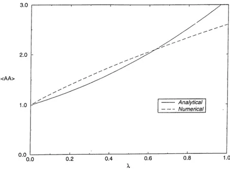
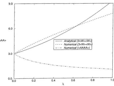
). The pure two-body correlations, as a function of coupling strength A, arising from this ground state of the Hamiltonian (3.28) is shown in figure (3.1) by the solid line. The Gaussian approximation of four-body correlations as a function of the coupling strength A is shown by poHd üne';.' in Hgnre (3 “^) The dashed lines in the figures were calculated by using the exact Hamiltonian (3.24) and diagonalizing it in the standard harmonic oscillator basis. The feasibility of our calculation requires that the Hilbert space is taken to be a finite dimensional truncation in the harmonic oscillator basis with the maximum allowed number of phonons N^ax =

1000

. The numerical diagonalization of the Hamiltonian (3.24) requires the matrix elements in the harmonic oscillator basis which are given by

m\Hr = iHo)r

= ( (2n -h 1) + (5n^ -h 4n -h 2

-)-( (n(n - l)(4n^ - n + 3))'^Sm,n-2

(31)

Figure 3.1; The two-body correlations as a function of coupling strength A.

+ {2{n -I- l)(n -f

2

)(

2

n^ -b

6

n -b

7

) )

2

<

5

m,n

+2

-b((n -b l)(n -b 2)(n -b 3)(n -b 4:)Ÿ^Sm,n+4

+ {n (n -b l)(n -b 2)(n -b 3) )2Sm,n-4^ (3.32) Ti;e numerical calcuiatiuns sauwu oy the dashed iiues in figures fS.l) and (3.2) were performed in the numerically calculated ground state .The numer ically calculated four-body correlations without the Gaussian approximation as shown by the dotted dashed lines in figure (3.2) differ significantly from those which were performed analytically and numerically using the Gaussian approximation.

We conclude that, for all couplings, it is not possible to ignore the pure four body correlations, i.e our method works but the approximation =

3y/l^y is highly unreliable. In the next section we will apply second and third order perturbation theory to extend the accuracy of our calculations in figure (3.2). Our calculations will be performed using the basis vectors corresponding the exactly solvable part of the Hamiltonian (.3.24) rather than the harmonic oscillator basis.

(32)

Figure 3.2: The four-body correlations as a function of coupling strength A.

3.3.1 Second and Third Order Time-independent Per

turbation

VVe shall start with the derivation of the perturbed Hamiltonian Hp. The fourth order correlations can be found by rewriting eqn.(3.11) as

(ÂiA2AÂ<^ = (ÂiA2A-iA,^ ^

(ÂiA'^lÂÂ^ -f- (Â\A:^(Â.2A.^ + Â

2

A

3

^ ^ /liA t) (3.33) The Gaussian approximate Hamiltonian (3.28) being the exactly solvable part of the Hamiltonian (3.24) is responsible of generating pure two-body correlations which are given by the three terms in the square bracket above. For the perturbed Hamiltonian we take the difference between the Hamilto nian (3.24) and (3.28). Hence the perturbed Hamiltonian is to be considered as (3.28).

(33)

Hp = {a^a + i ) + + X(A^ - 3XWA^)

Z --- ---^

"- - - ' V Ho

(3.34)

where A also becomes strength of .perturbation expressed.by eqn.(3.21). Now we start the same transformation technique in section 3.2.3 for the Hamiltonicin in eqn.(3.28). The transformation ,5'(<fo).i^P'S'^(<^o) leads to

Ep ^ Oo(M 6+ i ) + A,?(^o)[/l'‘ - 3 X W A % 9 % )

=

**+ ^) + A[e'*^'°(6 + 6^)4 _ 3Aft^e^^°(6 + M)^]**

(3.35)

where (fo is calculated self-consistently by eqn.(3.30) . The corrections to ground state due to the perturbation including the second order perturbation is given by I ~ ^ oo \Vnlr Ao = = AV^o + j j , ^ (3.36) fcyio

[E o - Ek)

where Vkj = (3.37)

with Eq^^ being the approximate ground state energy including the second or der corrections due to the perturbation, and Eq = being the exact ground state energy of the exactly solvable part rr^ lU cqii.(u.3oy. rn cqn.\^3.u7) denotes the excitation on the squeezed vacuum state |^o) given by

(3.38)

After a tedious algebra second order perturbed unrenormalized ground state

(3.39) energy can be found as

4 ^ ) = ii^o + Î3Ae'‘^° - 42^e®«°

and the second order perturbed ground state is given by

(34)

î7q (3.40) with the dimensionless renormalized phonon frequency given by

H o = + 1 ) . ( 3 . 4 1 )

The perturbed ground state vector (^

0

^ \ should be properly normalized as

= _{(l + § e 8io(G'2 + ,F2)) ■}eo) (2) (3.42) G = ( з ^ Æ + ^ ( 7 + 1 8 ^ / 2 ) ) , F - (

2

^ + A ( 2 1 + 8x/3 ) % where n = I 3a/ 9 4 -N

^0

' ' j such that ^ ^

We now have a normalized second order perturbed ground state energy as well as ground state which can be used in the analytic calculations in the second order perturbation to the pure two-body correlations. These are given by

= W + -^e^^°2V2G +

ÎLq Hq i-yS G .F + 5G’ + 9F^ (3.43) Using eqn.(3.36) we can calculate the first and the second perturbed correc tions to the Gaussicin approximation for the four-body correlations. These are presented in figure (3.3). A comparison of figure (

3

.

2

j with (3.3) yields that the second order correction to the Gaussian approximation becomes a better approximation to the Gaussia,n approximation itself. We can conclude that accuracy can be extended in the weak coupling range to A =

0.2

with the second order corrections to the Gaussian approximation.

.After making a similar analysis for the third order perturbation we find that the unrenormalized perturbed ground state is

,(3 )

ifo) — |<fo) + C n |(f2 ) +

Cl

2

-b -b <¿01411^8^^ — <^

12

) ) (’^•44:)

(35)

where constants are Cii = ( - 3 + - 27788^^ ci2 = (-.5 + 56<^ + 2341(^^)\/6 Ci3 = (7.7 - 2069<^) \/5 cu = (3 -237©)\/70 ci5 = 371\/7 ci

6

= 7 . 5 ^

The corresponding third order perturbed energy is

4 " ) = li7o li<f> + 482<^'

The normalization of is fixed by

where 1 N2 I + (f>^ c^-y + Cy2 + -f C

14

} + ^^{0^5 + 4 } (3.45) (3.46) (3.47)

The third order corrections to the Gaussian approximation for the four- body correlations can be found by calculating the third order corrections to two-body correlations as

/oCo

JV2 1 -I- 2\/2>p(cii)

(36)

+ 4\/3ciiCi2 4" 9cj2^

+(f>\2^M cnC iг)

+ ^ * ^ 1 3 c j 3 + 4 \/r 4 c i3 C i,i + 17cj^4^

— ¿"’ (Gx/IOCmCis

-\-(j)^ {21c\^ + 4\/33ci5Ci6 + 25cjg (3.48) The four-body correlations using (3.48) are also shown in figure (3.3). It is clear that the accuracy of the second order corrections can be increased by including the third order ones. On the other hand the connected part of the four-body correlations were not present in the Gaussian approximation. Those contributions arise from the difference between the four-body correla tions and their Gaussian approximation. Hence summation of the two curves

corresponding to and gives an approximation to

the numerically calculated four-body correlations which is also shown in the same figure.

(37)

Figure 3.3: The dependence ot the 2"“^ and the order corrections to the four-body correlations and the four-body cumulant with the 3’’“^ order cor rections as a function of coupling strength A.

(38)

Chapter 4 The Momentum Dependent

Quartic Hamiltonian:

A numerical approach

4.1 Introduction and Motivation

The motivation of the momentum dependent approach that we have intro duced in the previous chapter was based on simplifying the momentum- energy dependence of the ctnharmomc interaction by decoupling tlie con servation laws in the energy-momentum space. We have then introduced a scheme to further decouple the correlations corresponding to the Gaussian part of the interaction from the pure fourth order correlations. This allowed us to examine second and fourth order correlations separately. Our conclu sion based on figure (3.1) and (3.2) was that the Gaussian approximation to ciuartic interaction fails in the entire coupling constant rainge. On the other hand the perturbative corrections with order n based on the Gaussian approximation yields an increasing accuracy of the analytic calculations in comparison with the results obtained by direct numerical diagonalization. Flowever the perturbative corrections are not systematically easier to handle than the direct numerical results, moreover the accuracy of the perturbative corrections is limited to weak coupling constants A <

0

.

6

. These qualitative

(39)

results yielding a general understanding of the two and four particle córrela tions are expected to hold also in the momentum dependent case. Hence the upshot O Í the previous chapter is that one has to resort to pure numerical diagonalization techniques in the case of a momentum dependent interactions. The momentum dependent approach itself is crucial for understanding the thermodynamic behavior. In the momentum space in pcirticular the momen tum dependent interaction has exchange correlations which are not present in the momentum independent case. The importance of the exchange cor relations is to couple the thermodynamical behavior of the system which is leased on the energetic arguments with the momentum conservation in the presence of momentum dependent coupling. This is a crucial condition in understanding whether the interacting system goes through a ВЕС in the case of a canonical ensemble. This point, namely possible presence of ВЕС in the low temperature regime and its connections with exchange correlations was recently raised by Noziréres [15]. In this chapter we will devise a new numerical method in the diagonalization of momentum dependent quartic Hamiltonian.

4.2 Preliminaries For the Numerical Method

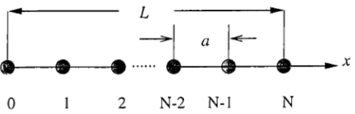
In chapter 2 we have introduced the abstract vector space for a many-body systems which is an infinite Hilbert space. In our one-dimensional lattice we have ions equally spaced with an inter-particle distance a. taking the inverse f the System also corresponds to an one·dimensional

lat-isfo..m o.

tice which is so called reciprocal lattice, which is sketched in figure (4.1) and figure (

4

.

2

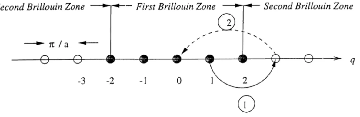
). This is a discrete system and we can say that ever}'· lattice site corresponds to a single state which is given in eqn.(2.16). This means that we represent site as where Ui is the number of particles at momen tum site. For numerical purposes we will take this lattice finite. The region between the boundaries will be the first Brillouin Zone, the interactions be tween other lattice sites which belong to second, third, etc. zones corresponds to the standard Umklapp processes (See figure (4.3)). This condition gives rise to periodic boundaries with periodicity given by the momentum Q corre sponding to reciprocal lattice constant, which is connected to the maximum number of sites in the first Brillouin Zone (i.e. the maximum momentum that a particle can have). The second restriction imposed by the feasibility of the numerical calculations is on the maximum number of phonons at

(40)

L

# --- ® --- · ... ® w ®

-0 1 2 N-2 N-I N

Figure 4.1: One-dimensional lattice in configuration space.

.

kI a

# ---1^

^

- 4 Q-3 Q-2 Q-1

Figure 4.2: One-dimensional reciprocal lattice in momentum space.

momentum site. We will assume that a site can contain at most Umax ps^rti- cles. Hence with these conditions our numerical technique will be based on a finite truncated Fock space. We are going to construct our abstract vectors on this space.

(41)

Figure 4.3: One-dimensional reciprocal lattice with cyclic boundaries. Ar rows sketch the Umklapp processes.

4.3 Mathematical Background

We will begin with construction of the abstract state vectors for the Hilbert space of our model Hamiltonian. As it was shown in eqn.(2.16) we can represent a single state as

'f(n i,n 2 . . . ,nQ) = n i n 2 ...n g ) .

In particular our occupation-number states are simply the direct product of the oi^i

5

lo inode number states

nxn2 . . . n g ) = |ni) (g) |n2) .. . (^) h e ) (4·^) In fact in an infinite abstract state vector space every single mode is unique, i.e. one single mode is counted once, but as our system has periodic bound ary conditions which should be properly implemented in to the numerical scheme. We now discuss our numerical approach starting with the following proposition.

Proposition 4.1 A single mode state can be uniquely represented as

n„_‘■

₇

₎

_(^7

₊

₁

_)'^

where n and q are integers which satisfy, 0 ^ q ^ Q rifnax

29

(42)

^0 'b-j

particles particles particles

q=0 q=l q=Q-l

Figure 4.4: A schematic representcition of our proposition, no particles situ ated cit slot

<7

=

0

etc...

and

0

< n <

The maximum number of particles Птах can occupy a particular mode and Cq{nq) = n,

4

-

1

is a coefficient for a particular mode state. Note also that К = Птах + 1· This implies that from a geometrical point of view we placed particles into horizontal slots (which corresponds to a single mode state) with every slot has a length of Umax + 1 and there are Q slots, as it is shown in figure (4.4).

Proof 4.1 i) Homomorphism :

By defining the analogue of (g) in our representation as A ® В = A + В ( —К^бд^д') , i.e we add two states if their modes are different and subtract ¡{{mode) they are same. Hence

n

(n + m +

1

) - f l {К У - (К У (n + m)g Homomorphism is trivial □

ii) One to one correspondence : Let, Пд)

-and, without loss of generality, we can assume that

q' > q

then we have,

[Ug 4- l)(Vlmaa; 4* 1)'^ = (^,,' 4” f)('nmai "h f)^

(43)

which implies,

riq +

1

< 7 T T — {^max H“

1

)

q ' - q

(4.3)

The largest value L.H.S could have is Umax·, i-e n, +

1

n'^i +

1

First case to be observed is

<7 > <l then R.H.S of eqn. (4.3) becomes

(rimax + i y , q = ( l ' - ( l >

we see that R.H.S is always greater than L.H.S which means that the equality given in (4.3) can never be satisfied. The other case is q' - q this is nothing but,

n, +

1

+

1

=

1

Which implies

n,

-Hence tne correspondence is one to one □

As a corrolaiy of the previous proposition, the representation wi i,nc rniucated many-body wave function ^ ( n i ,n

2

. . . ,n q -i) is

Q-i

n in

2

. ■. X ) C ,(n ,).(A )'’ (4.4)

This representation allows us to make calculations in a truncated Hilbert space. Taking the space finite causes some boundary effects such that if, be cause of the interaction, the number of particles exceeds Umax Ri' particular mode our system will ignore this situation and ^Lis will cause a negligible effect for a system in the low temperature regime. Now we should define the analogous creation (aj) and destruction (a,) operators of the abstract state

vector space in our representation.

(44)

D e fin itio n 4.1 VVe define the operators by their action on their basis states as

siA = { C i { n i ) - l f l ‘y A - K y

where first the operation in the curly brcicket is applied to the sum (state) then result is multiplied by the particular coefficient.

P r o p o s it io n 4.2 sj and s/ are the ancilogue operators of in this rep resentation.

P r o o f

4.2

VVe start with usual creation operator acting on abstract state

vector, a\ niri2 . . . n i . . . nQ_i s]C ,(n ,)IC {Clini)) 1/2 A" + Y , C ,(n ,)K ' q = 0

niri2 . . . (n; + 1)/ . . . riQ-i I—>■ (Cl(ni)j I ^2 Cyriq)K

\ q=0

<3-1

On the other hand

Similarly

5

, is analogue of a, in our representation Box.

(4.5)

4.4 Computational Technique

With these two operators at hand we will show step by step how we can implement this general formalism into a numerical scheme. Our aim is to take a vector and convert it to a number and then define the action of the

(45)

operators on this number as in proposition (4.2) cind finally convert back to a vector.

Let us consider n-max = 99, i.e {K —

100

), and Q = 3. This corresponds to a 3 site lattice in momentum space as shown in figure (4.3) where we can have maximum 99 particles at each site.

We now explciin this com.putatioruil technique by an example. Suppose thcit we have

10

particles at </ =

0

, 28 particles at i/ =

1

and no particles at

<[ — 2 state. Then the many-body state is described by

lO)

/ (7=0 28 (7=1

O)

' n=7 = 2 (4.6)

if this state is assigned to a number as in proposition (4.1) this unique number will correspond to

10000

)

Thermodynamic Quantities

Once the states and operators are constructed we can immedicitely represent our Hamiltonian in a matrix form and then by using standard diagonalization techniques we obtain the energy eigenvalues, £,· and eigenstates i), where

= (*|//|«)

~ ~b *^70^4n)~b

L 70 ^

^ Y2 M{qo, qi,q2, <7 3 ) ^ 0 ^

71

^

72

^^

7

3

+ <Zo + <7i + <'/2) } '·) (d.7) 4! _{7 i >72,73}

where hug^ = he. qo is the non-interacting energy of each mode with c

being a constant in dimensions of velocity, and A', iV/((?o, r/i, <

72

, r/

3

) ¿‘■re the interaction strength and function respectively.

In order to analyze the thermodynamical properties of this model system for fixed N , we will repeat the traditional analysis for free or interacting particles in a box

1

N = E rii■ ’ g i(.·.-») _

1

(4,8)

where

k eT

ks being Boltzmann constant and ^ is the chemical potential.

One can easily obtain the chemical potential by iteration, Irom eqn.(4.7) for a fixed N. At this level e,, 's are known as a result of dicigonalization process.

(77)^, the average internal energy of the system at a certain temperature is given by

{U )t — X ] _q₀₍_s_{, -}_m_{) —} (4.9)

(47)

Then for the heat capacity [Cy) one can use

(4.10)

The results which will he outcuned in the next section w ill be based on these numerical methods.

(48)

Chapter 5 The Low Temperature

Thermodynamics and a

Possibility of ВЕС for a Finite

and Discrete System

5.1 One-dimensional finite and Interacting

System

The semi-classical treatment of the condensation phenomenon is generally related to the concept of the density of states, p(e), where the system is con tinuous. Therefore in order to understand the thermodynamic properties of the system one can replace the sum given in eqn.(4.5) with an integral, where the energy eigenvalues are taken to be a continuous lunction of momentum and the integi'cil is taken over either in momentum space or in energy space as

J depie)·^_{,13(€-ц) _}1 = N. (5.1)

Hence the thermodyniimic properties ol the system can be obtained by tol- lowing the traditional analysis[-39].

(49)

100,0

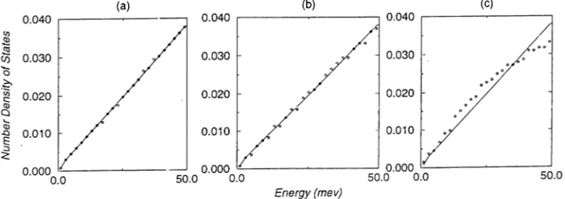
Figure 5.1: The density of states for (a)

77

= 2 (b)

77

= 1.5

If we consider a one-dimensional gas of identical bosons with mass m which are confined by a power-law potential U {x) = Uo{\x\/L)'^ then the density of states is given by

dx ^ / ^ /-/(d

= _ _ _ ^ ^

·- -d ^ > y e -U [X ,

(5.2)

where 2/(e) is the available length for bounded particles with energy e. Note that /(e) = It has been shown[ll][L3] that in one-dimension for

77

<

2

, yu reaches

0

at some temperature Tc- Such that the corresponding DOS behaves as

p{^) €

2

~ e (5..3)

with a =

1

/^ ~

1

/

2

.

Varying the exponent

77

one can make the integral given in (5.1) convergent leading to finite Tc- It is clear that

77

=

2

corresponds to a harmonic potential and the corresponding Tc vanishes. According to the DOS analysis, we can conclude that there is no BEG exhibited for a dynamically non-interacting system in the presence of an external harmonic potential. Figure (

5

.

1

.a) leads

Low-temperature thermodynamics of finite and discrete quartic quantum oscillator in one dimension

L O V V ^ ™

O F

# I N I №

-r

:,- ^ s u B M r i^ i0 T O 'T №

-

ND THE INSTlT!:]TE’0r;:ENGINEERiNG:3^N

IN PARTfttltJi;>FIlAMENTp THE REpumEMEN'TS^:

:,■ ' ^::· -FOR THE'HEGREE

’'

•

; -MASTER OF SCIENCE .

B y

A fif SlD D IK i

September 1999

LOW-TEMPERATURE THERMODYNAMICS OF

FINITE AND DISCRETE QUARTIC QUANTUM

OSCILLATOR IN ONE DIMENSION

By

A fif Siddiki

September 1999

ABSTRACT

LOW-TEMPERATURE THERMODYNAMICS OF FINITE

AND DISCRETE QUARTIC QUANTUM OSCILLATOR IN

ONE DIMENSION

Afif Siddiki

M.S. in Physics

Supervisor: Assistant Prof. Tuğrul Haldoğlu

September 1999

::3

7

ÖZET

AYRIK VE SONLU BİR BOYUTLU DÖRDÜNCÜL

KUANTUM SALINICISININ DÜŞÜK SICAKLIKTAKİ

TERMODİNAMIİK ÖZELLİKLERİ

Afif Sıddıki

Fizik Yüksek Lisans

Tez Yöneticisi: Yard. Doç. Tuğrul Hakioğlu

Eylül 1999

ACKNOWLEDGMENT

Contents

2.1

6

2.2

8

3.2

11

5

2.1

5

2.2

List of Figures

0

1

1

0

1

1

1

0.1

1

0.1

1

5.12

0.1

0

5

Chapter 1

Introduction

6

8

10

12

20

1

5

0

7

E

₂

₁₁

_(2.13)

₂

₂₀