Monetary policy in a Two–Agent New Keynesian (TANK) model with two sectors

(1)

MONETARY POLICY IN A TWO–AGENT NEW KEYNESIAN (TANK) MODEL WITH TWO SECTORS

A Master’s Thesis

by

ESER TUNA ERTEN

Department of Economics İhsan Doğramacı Bilkent University

Ankara September 2019

(2)

(3)

(4)

MONETARY POLICY IN TWO–AGENT NEW KEYNESIAN (TANK) MODEL WITH TWO SECTORS

The Graduate School of Economics and Social Sciences of

İhsan Doğramacı Bilkent University

by

ESER TUNA ERTEN

In Partial Fulfillment of the Requirements for the Degree of MASTER OF ARTS

DEPARTMENT OF ECONOMICS

İHSAN DOĞRAMACI BİLKENT UNIVERSITY ANKARA

(5)

(6)

ABSTRACT

MONETARY POLICY IN A TWO–AGENT NEW KEYNESIAN (TANK) MODEL WITH TWO SECTORS

Erten, Eser Tuna

M.A., Department of Economics

Supervisor: Asst. Prof. Dr. Burçin Kısacıkoğlu

September 2019

The objective of this study is to analyze the implications of consumer hetero-geneity for monetary policy in a setting simpler than a general heterogeneous agent model. I present a Two–Agent New Keynesian (TANK) model with two sectors, extending the “Limited Asset Markets Participation” (LAMP) model of Bilbiie (2008) by including a second sector based on Woodford (2003) and Woodford (2010) and, following Cravino, Lan, and Levchenko (2018), the possi-bility that expenditure shares are different for each household type. The model includes three sources of heterogeneity that have been shown to be relevant to policy (Cravino et al. (2018), Clayton, Jaravel, and Schaab (2018)): Two household types (called ‘poor’ and ‘rich’) that differ in their ability to smooth consumption, two final good sectors with different degrees of price stickiness and subject to different technology shocks and, unequal expenditure shares of each type for each final good. I also present a method of aggregation follow-ing Cravino et al.’s (2018) construction that makes it possible to express the model equations in a manner similar to that of the baseline three–equation

(7)

New Keynesian model. An analysis of impulse–responses under diﬀerent pa-rameter specifications reveal that the responses of variables when expenditure shares vary for each type are generally spread around the response when poor households’ share equals 0.5. I find that having a larger expenditure share for the relatively flexible price sector dampens the eﬀects of monetary policy on both the poor and rich households’ consumption compared to the case where the shares are equal.

(8)

ÖZET

İKİ SEKTÖRLÜ VE İKİ TÜKETİCİLİ YENİ–KEYNESÇİ BİR MODELDE PARA POLİTİKASI

Erten, Eser Tuna

Yüksek Lisans, İktisat Bölümü

Tez Danışmanı: Dr. Öğr. Üyesi Burçin Kısacıkoğlu

Eylül 2019

Bu çalışmanın amacı, tüketici heterojenliğinin para politikası üzerindeki etki-lerini genel bir heterojen tüketicili modele oranla daha basit bir kurulum ile incelemektir. Bu amaçla, Bilbiie (2008)’in “Limited Asset Market Participation” (LAMP) [“Kısıtlı Varlık Piyasası Erişimi”] modelini, Woodford (2003) ve Wood-ford (2010)’da anlatılan iki sektörlü modeli esas alıp genişleterek iki sektörlü ve iki tüketicili bir model sunmakta ve Cravino et al. (2018)’ın çalışmasını takip ederek söz konusu iki tür tüketicinin sektörel harcama paylarının farklı olması olasılığını da bu modele eklemekteyim. Model böylelikle Cravino et al. (2018) ve Clayton et al. (2018)’in gösterdikleri gibi politika için öneme haiz (i) tasar-ruf etme yetileri bakımından farklı iki hanehalkı türü (‘zengin’ ve ‘fakir’), (ii) nihai tüketim malı üreten ve fiyat değiştirme sıklıkları bakımından farklı iki sektör ve (iii) her bir nihai tüketim malı için her hane türünün farklı tüketim ağırlıklarını içermektedir. Buna ek olarak yine Cravino et al. (2018)’in göster-dikleri yöntemi takip ederek ekonomideki genel üretim ve tüketimi özetleyen bir toplama (aggregation) yöntemi sunmaktayım. Bu, modelin denklemlerinin

(9)

temel üç denklemli Yeni–Keynesçi bir modelde olduğu gibi ifadesini mümkün kılmaktadır. Farklı parametre değerleri kullanılarak elde edilen dürtü–tepkilerin incelenmesi, değişkenlerin harcama paylarının eşit olmadığı durumdaki tepkile-rinin harcama paylaından bitepkile-rinin %50 olduğu zaman elde edilen tepkilerin etra-fında dağıldığını göstermektedir. Harcama paylarının farklı olduğu durumda iki sektör arasındaki enflasyon farkını özetleyen değişkenin önem kazandığı ve böy-lece hanehalklarının tüketim tepkilerinin değiştiği gözlemlenmiştir. Görece daha sık fiyat değiştirilen sektörde daha büyük bir harcama payı bulunan hanehalkı-nın tüketiminin para politikasından payların eşit olduğu duruma göre daha az etkilendiği anlaşılmıştır.

Anahtar Kelimeler: Heterojen Tüketiciler, Para Politikası, Yeni–Keynesçi Mo-deller

(10)

ACKNOWLEDGMENTS

I would like to express my gratitude to my advisor Asst. Prof. Dr. Burçin Kısacıkoğlu for always being available for my many questions during the prepa-ration process of this thesis. I also would like to thank my second reader

Prof. Dr. Refet Gürkaynak for his comments. Professors Sang Seok Lee and Hüseyin Çağrı Sağlam have also kindly oﬀered their guidance whenever I con-tacted them for ideas on how to solve problems I have encountered in my work, for which I thank them.

(11)

LIST OF TABLES

1 Relation to Earlier Studies . . . 33 2 All Parameters of the Model . . . 35

(16)

LIST OF FIGURES

1. Responses to Monetary Policy I . . . 48

2. Responses to Monetary Policy II . . . 49

3. Responses to Monetary Policy III . . . 50

4. Extreme Case I . . . 51

5. Extreme Case II . . . 52

6. Responses to Sector 1 Technology Shock . . . 53

7. Responses to Sector 2 Technology Shock . . . 54

8. Expansionary Monetary Policy . . . 81

9. Responses for Various Shares of Poor Households (µ) . . . 82

(17)

CHAPTER 1 INTRODUCTION

Understanding monetary policy’s links to the economic behavior of households is important to improve its accuracy. Although policymakers often have to rely on aggregated data, which inevitably results in some loss of information, this does not imply that finer economic differences across households are unim-portant for how monetary policy works or how effective it can be. Households vary in terms of the income they earn and the wealth they accumulate, which can possibly be influential in how they respond to monetary policy. Recent re-search has shown that this is indeed empirically the case: Cravino et al. (2018) demonstrate the link between the position of a household in the income dis-tribution and its preferences for goods and study the effects that this link can have on policy. Considering a different dimension of consumer heterogeneity, Clayton et al. (2018) show that having college education also is associated with consumption of certain goods, which implies that the effects of policy will be different for each household.

Recent studies of the relationship between policy and the household hetero-geneity empirically supported by the two papers above is achieved by means of building models of the type known as Heterogeneous–Agent New Keynesian (HANK).1 _{In fact, both Cravino et al. (2018) and Clayton et al. (2018) employ}

(18)

a HANK–like model to incorporate to a theoretical framework the household heterogeneity that they have identified. The primary objective of this paper is to study this heterogeneity with a simpler model. To do this, I present a Two– Agent New Keynesian (TANK) model featuring two consumers and two final goods sectors, extending Bilbiie’s (2008) two–agent “limited asset market par-ticipation” (LAMP) model based on the two–sector representative agent one constructed in Woodford (2003) and Woodford (2010). Following Cravino et al. (2018), each consumer type has heterogeneous preferences over the final goods through unequal expenditure shares. I ask whether adding these sources of het-erogeneity changes the model’s predictions, and if so, to what extent. The first question is how adding the heterogeneity studied by Bilbiie (2008), namely, two types of households that diﬀer in their ability to smooth consumption, aﬀects the impulse–responses of the two–sector representative agent model. In this first case, I assume that the expenditure shares are equal for the two house-hold types. Next, I ask if there are further changes to the model’s predictions if expenditure shares are no longer equal. Lastly, I present the responses of all variables to technology shocks from either sector.

My choice of a two–agent model is for two reasons: First, the aim is to retain computational simplicity. The papers that employ a HANK model cited above necessarily use exogenous shocks particular to each household, which, together with a continuum of agents, necessitates simulations and numerical methods to obtain a solution. As will be seen, the two–agent model avoids these diﬃ-culties. As the two–agent model is a simplification of the many–agent one, it may be argued that some, possibly non–negligible, eﬀects associated with het-erogeneity will be lost. However, Debortoli and Galí (2018) has recently shown

two–agent, and the representative agent) and the respective abbreviations (HANK, TANK, and RANK) are due to Kaplan, Moll, and Violante (2018). The importance that the study of heterogeneity has gained in recent macroeconomic research is summarized in the review paper Galí (2018).

(19)

that this is not necessarily the case: Their baseline TANK model is able to de-liver impulse–responses that are closer to HANK and diﬀerent from the stan-dard RANK. Debortoli and Galí’s (2018) result therefore is the second reason to use a two–agent model. In addition to simplifying the model’s solution, us-ing a TANK model would also enable one to compare the resultus-ing impulse– responses with those in, e.g., Cravino et al. (2018) and Clayton et al. (2018) to assess its performance against these HANK–like models. In this manner, this paper also aims take the first steps to extend Debortoli and Galí’s (2018) exercise for a two–sector model with an additional source of consumer hetero-geneity.

This paper is not the first to develop a two–sector TANK model. In an ap-pendix to their paper, Clayton et al. (2018) do present a two–sector two–agent model, but my model here diﬀers from theirs in several respects. First, al-though they give a thorough analysis of their general HANK model, they do not explicitly study monetary policy or the eﬀects of technology shocks for their TANK model. Secondly, they assume perfect foresight and solve their model partly in continuous time. In contrast, the model here includes uncer-tainty and is in discrete time, as is usual in NK models. Thirdly, they assume that both household types receive an identical share of profits, and that each type is able to work in only one sector. Here, extending Bilbiie’s (2008) model, I assume that only the household type that is able to smooth consumption re-ceive profits (ie, they own all intermediate goods firms) and that both types of households supply labor in a labor market common to both sectors. Finally, I also show that aggregation of the model based on a set of assumptions is possi-ble, which their presentation does not include.

On the other hand, as also observed by Woodford (2003: p. 200), a two–sector model like the one I construct below is similar to an open economy model with two countries. Two open economy extensions of Bilbiie (2008) that is

(20)

simi-lar to the extension here are Eser (2009) and Boerma (2014). The main dif-ferences between these extensions and the one considered here are as follows: First and foremost, while they analyze open–economy questions, I consider a closed economy model. As is usual in open–economy models, in these two pa-pers labor is assumed to be immobile across countries, which translates in this model into all types of agents working in a single sector. As stated above, I assume that all agents are able to work in both sectors, that is, labor is mo-bile across countries, to use the open–economy language. Secondly, as the unit of study in open economy models is the ‘home country’, there usually is one Phillips equation for the domestic economy. In contrast, in the model I con-struct, since both sectors are a part of the same economy, there are two inter– connected Phillips curves, one for each sector. Finally, and more importantly, in both papers, the two types of households are assumed to have identical con-sumption baskets, ie, the weight of each good is the same for each household type. Following Cravino et al. (2018), I assume that weights for each household type diﬀer and study policy under that assumption. In an open economy two– agent context, this is equivalent to assuming that, in every country there are two types of agents who have diﬀerent levels of ‘home bias’ in goods.

I present the model in Chapter 2. I study the impulse–responses of all model variables to monetary policy shocks and technology shocks in Chapter 3. I con-clude in Chapter 4. I provide the auxiliary steps necessary to derive the equa-tions presented in the main text in the appendices.

(21)

CHAPTER 2 THE MODEL

As noted in the introduction, I follow Woodford (2003) and Woodford (2010) to construct the foundation of a two–sector model. I then assume that, fol-lowing Bilbiie (2008), in this economy of two final good sectors, there are two types of consumers that differ in their ability to smooth consumption and that only one type may receive dividends from the two sectors. These steps provide a two–sector closed–economy extension of Bilbiie (2008), open–economy ver-sions of which are due to Eser (2009) and Boerma (2014). The heterogeneity that I am interested in is the one documented and formalized by Cravino et al. (2018): Following their model, I further assume that the consumption baskets differ across household types. The source of this difference is, as in their paper, the unequal weights that each household type has for each final good.

2.1 Households and Consumption

2.1.1 The LAMP/TANK Structure

Following the LAMP model of Bilbiie (2008) and also its successor Debortoli and Galí (2018), I assume that two types of households whose sizes are invari-ant through time constitute the usual continuum of households. The two types diﬀer by their utility maximization problem in two respects: First, fraction

(22)

µ _{2 [0, 1] of households, whom I will call “poor households”, are assumed to be} unable to use financial instruments to smooth their consumption across time, whereas fraction 1 µ of households (the “rich households”) can participate in financial markets, in particular, they can own bonds and stocks.1 _{Bilbiie (2008)}

calls this structure the “limited asset market participation (LAMP)” model and it is also the foundation of Debortoli and Galí’s (2018) TANK. This is the first source of heterogeneity in the model.

2.1.2 The Two Sectors and Consumption Baskets

The second source of heterogeneity is the assumption that the consumption baskets of households are different. For example, one type may value a certain good more than the other type. To capture this in the simplest way possible, following Cravino et al. (2018), I assume that there are two final goods sectors (each using a continuum of intermediate goods produced by monopolistically competitive firms subject to Calvo–type price stickiness, with each sector hav-ing a different price stickiness parameter, to be detailed below) and that the households’ preferences on these two final goods vary as a result of each house-hold type having a different expenditure share on a given good. At the inter-mediate goods level, the model follows the standard NK modeling assumption: For each household type i, its final good j consumption, Ci

j,t, is assumed to be

a Dixit–Stiglitz aggregate of its consumption of intermediate goods, Ci j,t(k): C_j,ti ⌘ Z 1 0 C_j,ti (k)(⇣ 1)/⇣ ⇣/(⇣ 1) ⇣ > 1 (1.1)

where ⇣ is the constant elasticity of substitution for the intermediate goods.

1_{The naming of household types vary in each paper that utilizes this structure,}

depend-ing on the context. I prefer to label them “poor” and “rich” as I follow the income distribu-tion aspect studied by Cravino et al. (2018). Although the naming is diﬀerent, the type of heterogeneity introduced with this method is essentially identical in all studies.

(23)

An important question in a model with many sectors is the decision on the method of aggregation. Cravino et al. (2018), Clayton et al. (2018), and Wood-ford (2003: Chap. 3, Sec 2.5) use the most general constant elasticity of substi-tution (CES) form. To retain simplicity, I will follow the open–economy liter-ature and assume that aggregation is achieved by means of the Cobb–Douglas form2 _{for each consumer.}

Let the household types be indexed by i 2 {p, r}, where p stands for the “poor households” and r for the “rich households”. The final goods sectors are in-dexed by j 2 {1, 2}. I now introduce Cravino et al. (2018)–type heterogene-ity: Denote final good j’s share in the expenditures of household type i by ↵i

j.

Given the Cobb–Douglas aggregation assumption, the consumption index for household type i is Ci t ⌘ (Ci 1,t)↵ i 1(Ci 2,t)↵ i 2 (↵i 1)↵ i 1(↵i 2)↵ i 2 with ↵i 1+ ↵i2 = 1 (1.2)

2.1.3 Cost Minimization Problems

At the intermediate goods level and the final goods level, each type i solves standard cost minimization problems,3 _{which return the usual demand}

func-tions C_j,ti (k) =  Pj,t(k) Pj,t ⇣ C_j,ti (1.3)

2_{A special case of CES with the substitution parameter set to 1. The Cobb–Douglas}

form is the choice in, for example, Aoki (2001), Benigno (2004), Eser (2009), and Boerma (2014).

(24)

and C_j,ti = ↵i_j ✓ Pj,t Pi t ◆ 1 C_ti (1.4)

where Pj,t(k) is the price of intermediate good k in sector j and Pj,t is the price

of the sector j final good and the price indices are given by

Pj,t ⌘ Z 1 0 Pj,t(k)1 ⇣dk 1/(1 ⇣) (1.5) P_ti _{⌘ P}↵i1 1,tP ↵i 2 2,t i2 {p, r} (1.6)

The price index (1.6) is an indication of consumer heterogeneity, each house-hold type now has its own price index.

2.1.4 Defining Further Aggregate Variables

Using the demand relationships (1.3) and (1.4), I define expressions for aggre-gate variables in this subsection. More general forms of the relations derived here are given in Cravino et al. (2018), but I provide the (specialized) versions here for clarity and completeness. The main diﬀerences are that (i) a Cobb– Douglas form is used here and (ii) there are two consumer types of sizes µ and 1 µ, rather than Cravino et al.’s (2018) implicit assumption that household types are of the same size. Given the sizes of the poor and the rich, total ex-penditure on good j using the demand (1.4) can be written as

Pj,tCj,t = ↵jpµP p tC

p

(25)

The total expenditure on goods in the economy is then

P1,tC1,t+ P2,tC2,t = µPtpC p

t + (1 µ)PtrCtr (1.8)

Finding expressions for the aggregate price index Pt and aggregate

consump-tion index Ct is less straightforward. The diﬀerent weights on each good, as

will be seen later, lead to an expression diﬃcult to log–linearize. Cravino et al. (2018) use expenditure shares on each final good to define Pt and Ct, which I

follow here.4 _{This approach allows one to relate C}

j,t and Ct, as if there were a

cost minimization problem at the aggregate level. As shown in Appendix C.2, this relationship is given by

Cj,t = ↵j,t ✓ Pj,t Pt ◆ 1 Ct (1.9)

where following Cravino et al. (2018), the expenditure share of household i at time t, ei t is defined by ep_t _⌘ µP p tC p t µPtpCtp+ (1 µ)PtrCtr and er t ⌘ (1 µ)Pr tCtr µPtpCtp+ (1 µ)PtrCtr and ↵j,t ⌘ ↵pje p

t + ↵rjert. I note that equation (1.9) is a specialized version of

the equation with the same number in Cravino et al. (2018: p. 20). Equation (1.9) is the overall demand function for final good j and it is the expression one would obtain if there were an aggregate cost minimization problem. Given this, one can define the aggregate price index and the aggregate consumption index as

Pt ⌘ P1,t↵1,tP ↵2,t

2,t (1.10)

4_{The results in the rest of the subsection are also provided in Cravino et al. (2018), but}

once again for the more general CES case and without intermediate steps. I present the re-sults here and the derivations in the appendix nevertheless to motivate later discussion.

(26)

and Ct⌘ ✓ P1,t P2,t ◆↵2,t C1,t+ ✓ P2,t P1,t ◆↵1,t C2,t (1.11)

With some algebra, it can also be shown that indices (1.10) and (1.11) can also be defined equivalently in terms of household variables:

Pt= (Ptp)e p t(Pr t)e r t (1.12) and Ct = ✓ Ptp Pr t ◆er t µC_tp+ ✓ Pr t P_tp ◆ep_t (1 µ)C_tr (1.13)

The aggregate price index (1.10) is the specialized version of the more general one in Cravino et al. (2018: p. 20). They leave the aggregate consumption in-dex Ct undefined, here I have defined (1.11) so that equality across expressions

for aggregate expenditures obtains, that is

PtCt= P1,tC1,t+ P2,tC2,t = µPtpCtp+ (1 µ)PtrCtr (1.14)

It should also be stated that (1.13) is a generalized version of that defined by Eser (2009: p. 7)5_{. The diﬃculty, as remarked above, is that the share ↵}

j,t is

time dependent and a non–linear function, which make its log–linearization diﬃcult in later stages. One simplifying assumption is to use steady–state val-ues of ↵j,t as shares in the above equations, and to assume that (1.9) continues

to hold approximately when ↵j,t is replaced by its steady–state value. In that

5_{Eser (2009) considers the case without consumption basket heterogeneity (↵}p

j = ↵rj), in

(27)

case, as will be seen later, one has ep t = µ and ert = (1 µ), so that ↵j = µ↵pj + (1 µ)↵jr Pt = P1,t↵1P2,t↵2 (1.100) Ct = ✓ P1,t P2,t ◆↵2 C1,t+ ✓ P2,t P1,t ◆↵1 C2,t (1.110) Ct= ✓ P_tp Pr t ◆1 µ µC_tp+ ✓ Pr t Ptp ◆µ (1 µ)C_tr (1.130₎ and Cj,t ⇡ ↵j ✓ Pj,t Pt ◆ 1 Ct (1.15)

Then the specialized aggregate indices (1.100_{) and (1.11}0_{) can be used to}

de-rive an aggregate Euler equation for the economy and also the natural levels of output. I will first refrain from making the assumption that the shares are constant and solve the model without any assumptions on the economy–wide aggregates, except for when writing a Taylor rule for policy. This enables me to obtain a complete solution with minimal assumptions, but at the cost of fore-going the derivation of an aggregate Euler equation and also the natural rate of output. Then, in subsection 2.6, I solve the model once again, having made the assumption.

(28)

2.1.5 Utility Maximization Problems

I now add the properties peculiar to each household type. As in Bilbiie (2008), the main diﬀerence between the two household types is most visible in their budget constraints. Additionally, the unequal weights of the two types comple-ment the original heterogeneity stemming from the diﬀerential financial access in this case. Following Debortoli and Galí (2017: p. 11–12), I assume that the budget constraint of the poor household is

PtpCtp  WtNtp (1.16)

and the rich households’ budget constraint is

P_trC_tr+ Bt+ QtHt WtNtr+ (1 + it 1)Bt 1+ (Qt+ Dt)Ht 1 (1.17)

where Wt is the nominal wage rate (competitively determined in a common

labor market), Bt denotes the amount of bonds with risk–free return (1 + it)

held by the rich household in period t, it is the nominal interest rate in period

t (the policy rate of the central bank), Ht denotes the amount of shares held

at time t, each share having the price Qt, and Dt is the dividends that the rich

household receives from the intermediate good producers. The two constraints (1.16) and (1.17) are in fact specialized versions of the constraints constructed in Bilbiie (2008: p. 166–167). As noted previously, the heterogeneity arising from the varying valuations of goods of each household type manifests itself in the consumption expenditures: In the budget constraint of each type i, the relevant price index Pi

t, rather than an aggregate price index Pt appears.

(29)

Bil-biie (2008) once again to set

U (C_ti, N_ti) = ln C_ti (N

i t)1+

1 +

As is usual in standard New Keynesian models, I assume that both types of households have the same discount factor 2 [0, 1). The utility maximization problem of the poor household is then

max C_tp,N_tpE0 1 X t=0 t  ln C_tp (N p t)1+ 1 + subject to Pp tCtp  WtNtp (1.18)

As a result of the assumed form of the budget constraint, the poor households’ behavior will be what is known as “hand–to–mouth” in the literature: Solving problem (1.18) yields the optimality conditions

Wt

Ptp

= C_tp (1.19)

Ntp = 1 (1.20)

The labor supply of the poor household is therefore always inelastic, as in Bil-biie (2008), Eser (2009), and Boerma (2014). This facilitates the algebra as shall be seen later, which becomes even more important with the inclusion of a second sector. Next, consider the problem of the rich household:

max Cr t,Ntr,Bt,Ht E0 1 X t=0 t  ln C_tr (N r t)1+ 1 + subject to Pr tCtr+Bt+ QtHt WtNtr+ (1 + it 1)Bt 1+ (Qt+ Dt)Ht 1 (1.21)

The rich households are therefore those whose behavior is similar to the usual representative agent of New Keynesian models. Solution of problem (1.21)

(30)

gives the optimality conditions Wt Pr t = C_tr(N_tr) (1.22) 1 = Et  Pr tCtr Pr t+1Ct+1r (1 + it) (1.23)

and, after the equilibrium conditions (to be discussed later) are imposed,

P_trC_tr = WtNtr+

Dt

1 µ (1.24)

where one can define the stochastic discount factor (SDF), ⇠t,t+1 as

⇠t,t+1 ⌘ Pr tCtr Pr t+1Ct+1r (1.25)

which is a version of the one–period SDF defined in Debortoli and Galí (2018: p. 26). The significance of the SDF here can be summarized as follows: While the SDF is a function of the rich households’ expenditure as in Debortoli and Galí (2018), due to the varying expenditure shares across each household type, the rich households’ price index Pr

t and the overall index Pt no longer coincide.

Hence it is the rich households’ price index Pr

t that appears in the SDF’s

defi-nition and not the overall index Pt. As in Debortoli and Galí (2018), since the

intermediate goods producers are assumed to be owned by the rich households, they use this SDF (as opposed to an economy–wide one) when discounting fu-ture profits.

2.2 Firms and Production

The foundation of the production side of the economy is Woodford’s two–sector representative agent model (Woodford, 2003: Ch. 3, Sec. 2.5). I make two

(31)

sim-plifying assumptions: First, I eliminate his inclusion of sector sizes, and assume that the two final goods sectors are of the same size (in each final good sector, there is a continuum of intermediate goods producers, indexed by k 2 [0, 1]).6

Second, I assume a common labor market, rather than his “diﬀerentiated labor markets” (a specific competitive labor market for each producer k).7 _{On the}

other hand, adapting Bilbiie’s (2008) two–agent framework on the consumer side also requires following his assumption that there is a fixed cost for the in-termediate goods producers (which results in dividends received from interme-diate goods producers being zero at the steady–state) once again for the ob-jective of creating a simple model. Accordingly, let the production function for intermediate goods producer k in sector j, whose output is denoted by Yj,t(k)

be

Yj,t(k) = Aj,tNj,t(k) Kj (2.1)

where I follow Woodford (2003) and Woodford (2010) to assume that there are sector–specific temporary technology shocks Aj,t, and Kj > 0 is the fixed cost

of Bilbiie (2008).

2.2.1 Problem of the Aggregators in each Final Good Sector

For each sector j, the aggregator’s problem is standard. As is usual, I assume that the sector j final good Yj,t is a Dixit–Stiglitz aggregate of intermediate

6_{As will be seen, the sizes of sectors in the model will be determined by expenditure}

shares averaged across household types (↵j’s), rather than predefined sizes.

7_{As discussed in detail by Woodford (2003: p. 144 and Ch. 3, Sec. 1.4), the}

“diﬀerenti-ated labor markets” assumption introduces “strategic complementarities” in pricing to the model, which acts as an additional element that reinforces price stickiness. While according to Woodford (2003), this would bring a model closer to reality, it makes algebraic operations very diﬃcult in the model considered here. Therefore, I opt to assume a common labor mar-ket as it simplifies all the algebraic operations greatly.

(32)

goods Yj,t(k): Yj,t= Z 1 0 Yj,t(k)(⇣ 1)/⇣dk ⇣/(⇣ 1)

with the usual demand function implied by a standard profit maximization problem8 Yj,t(k) =  Pj,t(k) Pj,t ⇣ Yj,t (2.2)

and the price index Pj,t defined by (1.5).

2.2.2 Real Marginal Costs and Profits of Intermediate Good Pro-ducers

Following Woodford (2003: Ch. 3, pp. 148–149), I will first find an expression for real marginal costs and then define the profit function for intermediate goods producers. Consider an intermediate good producer k operating in sec-tor j. As it appears in (2.1), the firm’s demand for hours of work is Nj,t(k).

Given the assumption that there is a common labor market with a perfectly competitive wage per hour Wt, the nominal labor cost of the firm is WtNj,t(k).

This can be rewritten in terms of output of the firm using (2.1), implying that the nominal marginal cost of the firm is

Wt

Aj,t

Now one must choose a price index to divide the nominal marginal cost by to obtain the real marginal cost of this firm. In this case, the choice is not as clear as those in representative agent models or in two–agent models with identical

(33)

consumption basket shares. Here I argue that, as the firms are assumed to be owned by the rich households and the dividends (ie, the firms’ profits) directly enter their budget constraint, real marginal costs and profits must be obtained by dividing by the rich households’ price index Pr

t. Hence the real marginal

cost in sector j, denoted by MCj,t,9 is defined by

M Cj,t ⌘

Wt

Aj,tPtr

(2.3)

An alternative definition is used by Clayton et al. (2018), who define real marginal cost in each sector by dividing the nominal marginal cost by the price index of that sector. Their choice is apparently for simplification, but for the model considered here, that assumption would be hard to justify due to the argument just made.

On the revenue side, the intermediate producer k in sector j produces the amount Yj,t and sells it for Pj,t(k) per unit. Again following Woodford (2003),

nominal profits of the firm, denoted Dj,t(k), can be written, using (2.2) and the

real marginal cost expression (2.3), as

Dj,t(k) = Pj,t(k)1 ⇣Pj,t⇣Yj,t M Cj,tPtr

h

Pj,t(k) ⇣Pj,t⇣ Yj,t+ Kj

i

(2.4)

This form of profits is standard, except for the choice of the price index, dis-cussed just above.

9_{This is actually the real marginal cost for each firm k. This is a standard result of the}

assumption of a common labor market: All producers in a sector have the same real marginal cost. Marginal costs do diﬀer across sectors, but this is only due to the diﬀerent technology variables Aj,t.

(34)

2.2.3 Profit Maximization under Calvo Pricing

As in Woodford’s (2003) two–sector model, the two sectors in this model diﬀer because of two factors: (i) a technology variable particular to each sector (Aj,t)

and (ii) diﬀerent degrees of Calvo–type price stickiness. The latter is summa-rized by the usual parameters ✓j, j 2 {1, 2}, which denote the probability that

a firm k in sector j is unable to change its price in any given period. Under this price rigidity assumption, the profit maximization problem of an interme-diate good producer k in sector j is

max P⇤ j,t Et 1 X s=0 ✓s_j⇠t,t+s n (P_j,t⇤)1 ⇣P_j,t+s⇣ Yj,t+s M Cj,t+sPt+sr h (P_j,t⇤) ⇣P_j,t+s⇣ Yj,t+s+ Kj io (2.5)

The first order conditions, together with substitution for the SDF ✓j and

can-cellations and some algebraic manipulation give

P_j,t⇤ = ✓ ⇣ ⇣ 1 ◆ Et 1 X s=0 ( ✓j)s(Ct+sr ) 1P ⇣ j,t+sYj,t+sM Cj,t+s Et 1 X s=0 ( ✓j)s(Ct+sr ) 1P ⇣ j,t+sYj,t+s(Pt+sr ) 1 (2.6)

As is the case in standard New Keynesian models, log–linearization of this equation leads to the Phillips curve for sector j.

(35)

2.3 Market Clearing Conditions and Equilibrium

2.3.1 Market Clearing in the Goods Markets and the Labor Market

At the intermediate goods level, the supply of and the demand for good k are equal if

Yj,t(k) = µCj,tp (k) + (1 µ)Cj,tr (k) (3.1)

Likewise, for the final good j, one must have

Yj,t = Cj,t ⌘ µCj,tp + (1 µ)Cj,tr (3.2)

Turning to the labor market, the total supply of labor, Ns t, is

N_ts _{⌘ µN}_tp+ (1 µ)N_tr (3.3)

Assuming a common market for labor also means that one is assuming that there is a single type of labor in this economy. Hence the demands of each in-termediate good firm can be added (in fact integrated) to obtain the aggregate demand in each sector:

N1,t ⌘ Z 1 0 N1,t(k)dk and N2,t ⌘ Z 1 0 N2,t(k)dk

and then these can also be added to obtain the aggregate labor demand, Nd t:

(36)

The labor market clearing condition therefore is the equation (3.3) = (3.4):

N_ts = N_td (3.5)

2.3.2 Equilibrium in Financial Markets

There are two financial markets in this economy: The market for bonds and the market for stocks. As shown by Bilbiie (2008) and Boerma (2014), equilib-rium in these markets yield the conditions:

Bt= 0 and Ht=

1

1 µ (3.6)

that is, no bonds are held in equilibrium (no savers or borrowers) and each rich household owns an equal amount of stock in intermediate goods firms.

2.3.3 Aggregate Production and Aggregate Dividends

For a firm k in sector j, the production function is (2.1). Using the demand function (2.2) for Yj,t(k), one can aggregate the production function in sector j

(details to be provided later) by integration:

j,tYj,t = Aj,tNj,t Kj (3.7)

where the variable

j,t ⌘ Z 1 0  Pj,t(k) Pj,t ⇣ dk

is referred to as the “price dispersion” in the literature (Bilbiie, 2008: p. 168) (Galí, 2008: Ch. 3, p. 46). Details of aggregation of dividends are provided in Appendix C.1.

(37)

2.4 Log–Linearization of the Model

Steady–state values necessary for log–linearization of the model are derived in Appendix B. I use a convention common in the literature and denote the percentage deviation (or equivalently log deviation) of any variable Xt from its

steady state value by ˆXt+1 throughout.10

2.4.1 The Rich Households’ Euler Equation

I first log–linearize the intertemporal optimality condition (1.23) of the rich household. The log–linear version of the equation is

ˆ Cr t = Et( ˆCt+1r ) h ˆit Et(⇡t+1r ) i (4.1)

where ˆit⌘ it ( log( )) and ⇡rt ⌘ log Ptr log Pt 1r . Equation (4.1) is known as

the Euler equation. As also demonstrated by Debortoli and Galí (2018: pp. 5– 6), the equation is valid only for rich households, hence it is not an ‘aggregate’ Euler equation.

2.4.2 Consumption of the Poor Households

Log–linearization of (1.19) and (1.22) about their steady state values and com-bining the resulting equations to eliminate ˆWt yields an expression for the poor

households’ consumption, which can be written in terms of the relative price

10_{Linearization is about a steady state where there is zero inflation. Hence for the}

infla-tion variables, the actual value and the deviainfla-tion from steady–state coincide. Therefore I do not use the hat notation for inflation variables below.

(38)

variable ˆpR

t (defined in the next subsection) as

ˆ

C_tp = (↵p₁ ↵r₁)ˆpR,t+ ˆCtr+ Nˆtr (4.2)

In equation (4.2), the right–hand side is in fact equal to the real wage of the poor household (log–linear expression for nominal wage Wt divided by the poor

household’s price index Pp

t). The real wage of the poor household can be

ex-pressed as a function of rich household variables as a result of the common la-bor market assumption.

2.4.3 New Keynesian Phillips Curves

To obtain the New Keynesian Phillips curves of the two sectors in this econ-omy, one has to log–linearize equation (2.6). Following the linearization ap-proach outlined in Woodford (2003), I show Appendix C.4 that the Phillips curves for the two sectors are

⇡1,t = Et(⇡1,t+1) + (1 ✓1)(1 ✓1) ✓1 ⇣ d M C1,t+ ↵r2pˆR,t ⌘ (4.3) and ⇡2,t = Et(⇡2,t+1) + (1 ✓2)(1 ✓2) ✓2 ⇣ d M C2,t ↵r1pˆR,t ⌘ (4.4)

where, again following Woodford (2003: p. 203), I have defined ˆpR,t ⌘

log(P2,t) log(P1,t).

2.4.4 Households’ Inflation Rates

Given the multiplicative structure of all price indices and defining the inflation rate for household type i as ⇡i

(39)

that

⇡_ti = ↵₁i⇡1,t+ ↵i2⇡2,t (4.5)

2.4.5 The Goods Market Clearing Condition

Log–linearization of the goods market clearing condition (3.2) followed by a se-ries of intermediate steps detailed in Appendix C.3 lead to the linear equations

ˆ Y1,t = ↵r2pˆR,t+ ˆCtr+ µ ↵p₁ ↵1 ˆ N_tr (4.6) and ˆ Y2,t = ↵r1pˆR,t+ ˆCtr+ µ ↵p₂ ↵2 ˆ N_tr (4.7)

2.4.6 The Labor Market Clearing Condition

One can write (3.5) as

µ + (1 µ)Nr

t = N1,t+ N2,t

Log–linearizing this equation then gives

ˆ Ntr = ↵1 1 µNˆ1,t+ ↵2 1 µNˆ2,t (4.8)

(40)

2.4.7 Aggregate Production in Sector j

Log–linearization of (3.7) gives a log–linearized labor demand equation in each sector j: ˆ Nj,t = ✓ ⇣ 1 ⇣ ◆ ˆ Yj,t Aˆj,t (4.9)

2.4.8 Real Marginal Cost as Deviation from Steady State

In Appendix C.5, I show that the log–linearized real marginal cost equation for sector j firms is d M Cj,t = ˆCtr+ 1 µ ✓ ⇣ 1 ⇣ ◆ (↵1Yˆ1,t+ ↵2Yˆ2,t) 1 µ(↵1Aˆ1,t + ↵2Aˆ2,t) Aˆj,t (4.10)

2.4.9 Woodford’s (2003) Law of Motion for the Relative Prices

As shown in Woodford (2003: p. 204), a law of motion can be found for ˆpR,t

with straightforward algebraic operations: Given the definition of ˆpR,t, it can

alternatively be written as

ˆ

pR,t= ˆpR,t 1+ ⇡2,t ⇡1,t (4.11)

Equation (4.11) is equation (2.28) in Woodford (2003: p. 204).

2.4.10 Laws of Motion for Technology Shocks

As is usual in simple New Keynesian models (see, e.g. Galí (2008: Ch.3)), I assume that the technology shocks follow a (stationary) AR(1) process, but

(41)

the persistence parameters are diﬀerent across sectors. In log–linear terms, the equation for the sector j technology variable is

ˆ

Aj,t = ⇢jAˆj,t 1+ ✏j,t |⇢j| < 1 (4.12)

2.5 Monetary Policy

Following the standard assumption in the literature in general and Galí (2008: Ch. 3), Debortoli and Galí (2018), and Cravino et al. (2018) in particular, I will assume that the central bank follows a simple type of Taylor rule. It is the components of the Taylor rule that I have to be particular about. Since I have not yet defined the output gap as the diﬀerence between output and its natu-ral level, I will assume that the the deviation of ovenatu-rall output from its steady state value enters the rule, rather than the output gap. In addition, I define this overall output as the weighted average of the output from the two sectors:

ˆ

Yt= ↵1Yˆ1,t + ↵2Yˆ2,t (5.1)

On the other hand, perhaps the more important question is what measure of inflation should be in the interest rate rule, as options are now several (⇡1,t, ⇡2,t, ⇡pt, or ⇡rt). To remain close to the baseline models, I will assume that

this measure is, as in the case of output, a weighted average of inflation rates from the two sectors. I denote this average by ⇡t, and define it as

⇡t= ↵1⇡1,t + ↵2⇡2,t (5.2)

The Taylor rule for this model is therefore

(42)

where vt is the variable associated with the monetary policy shock:

vt= ⇢vt 1+ ✏t (5.4)

I note here that the overall output measure ˆYt and the overall inflation rate

variable ⇡t are posited without reference to optimization conditions of

house-hold types. As discussed in subsection 2.6.9 below, these variables will be con-nected to model equations once I make the extra aggregation assumptions (see subsection 2.1.4) and define all variables associated with flexible prices. Finally, one can use the well–known “Fisher equation” to define the deviation of the ex– ante real interest rate from its steady state value, ˆrt, as

ˆ

rt= ˆit Et(⇡t+1) (5.5)

As the rich households now have their own consumption basket, their real in-terest rate can be argued to diﬀer from the one just defined. I define the rich households’ real interest rate, ˆrr

t as

ˆ

rr_t _{⌘ ˆi}t Et(⇡t+1r ) (5.6)

The equations derived up to this point can be collected to form a linear ratio-nal expectations system of the Blanchard and Kahn (1980) type. Equations of this version of the model are summarized in Appendix E.1.

2.6 Economy–Wide Aggregation and the Natural Level of Output

As noted at the end of subsection 2.1.4, assuming that equations (1.100_),

(1.110_{), and (1.15) hold makes further aggregation possible, by making an}

economy–wide output variable Yt and therefore the ‘output gap’ (the

(43)

sec-tion, I find the natural level of output, relate the consumption index of the rich households to overall consumption and then to aggregate output. This enables me to write an aggregate Euler equation and to rewrite the Phillips curve re-lationships (4.3) and (4.4) in terms of the output gap variable, as is usual. Ag-gregation steps in this section (and its appendix) follow Bilbiie (2008), while the natural level of output is found by applying the steps outlined in Wood-ford (2003: Chapter 3, Sections 1–3 and Appendix B.7). I use superscript n to denote natural (flexible price) quantities, as is common in the literature.

2.6.1 Profit Maximization Problem of Firm k in Sector j when Prices are Flexible

If all prices are assumed to be flexible, in each period t, firm k in sector j needs to solve the problem

max Pj,t(k) Dj,t(k)⌘ Pj,t(k)1 ⇣Pj,t⇣ Yj,t M Cj,tPtr h Pj,t(k) ⇣Pj,t⇣Yj,t+ Kj i (6.1)

The first–order condition for this problem gives the optimality condition

Pn j,t(k) P_tr,n = ✓ ⇣ ⇣ 1 ◆ M C_j,tn (6.2)

The two sides of equation (6.2) can be rewritten by means of substituting vari-ables to obtain an expression that defines the natural level of output. The expression for the natural level of output can then be used to write the real marginal cost in sector j as a function of actual and natural levels of output. These steps are detailed in Appendix C.6. As shown below, log–linearization of the resulting equations ((C.6.3) and (C.6.4) in the same appendix) gives an expression for the natural rate of output ˆYn

t and an expression for dM Cj,t to

(44)

2.6.2 Log–Linearization of Aggregate Relationships

In Appendix C.7, I show that the log–linearized versions of the assumed aggre-gate relationships (1.110_{) and (1.13}0_{) imply that}

ˆ

Ct= ↵1Cˆ1,t+ ↵2Cˆ2,t (6.3)

and

ˆ

Ct = µ ˆCtp+ (1 µ) ˆCtr (6.4)

Note also that, if one defines aggregate output Yt by equation (1.110) with Cj,t

replaced with Yj,t, then, together with the market clearing conditions, equation

(6.3) implies that

ˆ

Yt= ↵1Yˆ1,t + ↵2Yˆ2,t (6.5)

This equation also holds when prices are flexible, that is,

ˆ

Y_tn = ↵1Yˆ1,tn + ↵2Yˆ2,tn (6.6)

2.6.3 Finding an Expression for ˆCtp

I replace ˆNr

t in (4.2) by using (3.5) and (4.9) to obtain an expression for ˆC p t.

After a few algebraic steps, the resulting equation is

ˆ Ctp = (↵p1 ↵r1)ˆpR,t+ ˆCtr+ ₁ _µ ✓ ⇣ 1 ⇣ ◆ (↵1Yˆ1,t+ ↵2Yˆ2,t) 1 µ(↵1Aˆ1,t+ ↵2Aˆ2,t) (6.7)

(45)

2.6.4 The Aggregate Euler Equation

It is shown in Appendix C.8 that the aggregate Euler equation for this econ-omy can be written as

ˆ Xt = Et( ˆXt+1) µ(↵p₁ ↵r 1)_[E t(ˆpR,t+1) pˆR,t] + ✓ µ 1 µ ◆ 1 h ↵1Et( Aˆ1,t+1) + ↵2Et( Aˆ2,t+1) i 1 hˆit Et(⇡rt+1) Et( ˆYt+1n ) i (6.8) where, following Bilbiie (2008), I have defined the parameter as

⌘ 1 µ 1 µ ✓ ⇣ 1 ⇣ ◆

and, as is standard in the literature11_{, ˆ}_X

t ⌘ ˆYt Yˆtn denotes the output gap,

the diﬀerence between the actual and natural levels of output. Equation (6.8) is the aggregate Euler equation for the economy considered in this study.

2.6.5 Labor Market Variables

Combining (4.8) and (4.9), one can write the labor supply of the rich house-hold as ˆ N_tr = 1 1 µ ✓ ⇣ 1 ⇣ ◆ (↵1Yˆ1,t+ ↵2Yˆ2,t) 1 1 µ(↵1Aˆ1,t+ ↵2Aˆ2,t) (6.9) Defining the real wage rate for the rich households by !r

t ⌘ Wt/Ptr, log–

linearization of the first order condition (1.22) gives

ˆ

!_tr = ˆC_tr+ Nˆ_tr (6.10)

(46)

As in Bilbiie’s (2008) study, these equations are of importance to analyze the labor market movements in the economy.

2.6.6 A Log–Linearized Expression for the Natural Level of Output

Appendix C.9 provides the steps to derive an expression for the natural level of output as deviation from its steady state, which ultimately yield the equation

ˆ Y_tn= ⇣[µ(↵ p 1 ↵r1) ↵2r] ⇣ + (⇣ 1) pˆ n R,t+ ⇣ ⇣ + (⇣ 1)(↵1Aˆ1,t + ↵2Aˆ2,t)+ ⇣ ⇣ + (⇣ 1)Aˆ1,t (6.11)

2.6.7 Restatement of the Phillips Curves

Phillips curves for the two sectors have already been given above, but alter-native versions of the two curves can be found by replacing the real marginal costs with the output gap variable. I present the details in Appendix C.10, which show that the Phillips curves (4.3) and (4.4) can be rewritten as

⇡1,t = Et(⇡1,t+1) + 1  ⇣ + (⇣ 1) ⇣ Xˆt+ 1↵ r 2(ˆpR,t pˆnR,t) 1µ(↵p1 ↵r1) ˆpR,t pˆnR,t (6.12) and ⇡2,t = Et(⇡2,t+1) + 2  ⇣ + (⇣ 1) ⇣ Xˆt 2↵ r 1(ˆpR,t pˆnR,t) 2µ(↵p1 ↵r1) ˆpR,t pˆnR,t (6.13)

(47)

where, following Woodford (2003: p. 208), I defined the parameter j as

j ⌘

(1 ✓j)(1 ✓j)

✓j

j _{2 {1, 2}}

for compact notation. The Phillips curve equations (6.12) and (6.13) can be viewed as generalizations of those in Woodford (2003: Prop. 3.8, p. 203), Bil-biie (2008: p. 173), and Eser (2009: p. 16). Firstly, they diﬀer from the two– sector representative agent model of Woodford (2003) in that the coeﬃcient of the relative price term (ˆpR,t pˆnR,t) is the rich households’ shares (↵rj), as

op-posed to economy–wide shares (↵j). This is the direct eﬀect of assuming that

there are two types of households. The equations here also generalize those in Bilbiie (2008) and Eser (2009) as a result of the last term that appears in the two equations, which captures the eﬀect of the the unequal shares of the house-hold types (↵p

j 6= ↵rj). One should note that, in the event that there are no

poor households in the economy (µ = 0), the last term disappears and ↵1 = ↵r1

holds, hence the equations reduce to those in Woodford’s (2003) two–sector RANK model.

2.6.8 An Expression for Woodford’s (2003) Natural Relative Price Variable

As in subsection 2.4.9, I also need an expression for pn

R,t to complete the model.

Such an expression can be found by subtracting (C.9.3) from (C.9.4) (in the appendix), which yields

ˆ

(48)

2.6.9 Monetary Policy in the Aggregated Model

Having an aggregate Euler equation and an expression for the natural level of output, I can modify the monetary policy rule. First, the equations (5.1) and (5.2) are now no longer postulates but equations derived from the aggregation assumptions. I therefore replace ˆYt with ˆXt in (5.3) to obtain the policy rule

ˆit= ⇡⇡t+ xXˆt+ vt (6.15)

As was the case at the end of Section 2.5, the derivations in this section pro-vides one with a model of linear equations which can be solved either by hand or with computer software. Equations of this second model with the aggrega-tion assumpaggrega-tions are summarized in Appendix E.2.

(49)

CHAPTER 3 RESULTS

3.1 Relation to Other Models

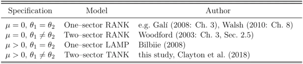
The model in this study extends those on which it builds upon. Hence one can obtain the results of the underlying models as special cases of the model here by setting the free parameters in Table 2 to particular values. Before moving on to the calibration of parameters in the next section, I present some of those cases in Table 1.

Table 1: Relation to Earlier Studies

Specification Model Author

µ = 0, ✓1 = ✓2 One–sector RANK e.g. Galí (2008: Ch. 3), Walsh (2010: Ch. 8)

µ = 0, ✓1 6= ✓2 Two–sector RANK Woodford (2003: Ch. 3, Sec. 2.5)

µ > 0, ✓1 = ✓2 One–sector LAMP Bilbiie (2008)

µ > 0, ✓1 6= ✓2 Two–sector TANK this study, Clayton et al. (2018)

3.2 Calibration

As noted above, although the validity of the relationships between economy– wide aggregate variables is dependent on the extra assumptions I have made, they have no bearing on the variables derived prior to aggregation (the first

(50)

version of the model).1 _{As the second version of the model comprises all}

vari-ables (economy–wide and more specific), I therefore use it for analysis hence-forth. However, I stress once again that the natural level of output and hence the output gap depend on the additional assumptions made, while the deriva-tions before them are independent of the latter assumpderiva-tions. The parameters that are peculiar to the model of this study are the expenditure shares of dif-ferent consumer types (↵i

j), price stickiness parameters of the two sectors (✓j),

and the share of poor households in the continuum (µ). I discuss the impli-cations of the model when these values vary, hence these parameters can be viewed as ‘free’. For the rest, I use the calibrated parameter values given for the baseline model by Galí (2008: p. 52). Table 2 summarizes all parameter– related information. Before moving on to the analysis of impulse–responses, a discussion of the calibrated values is necessary to motivate the baseline choices for parameter values reported in Table 2. I do this in the next two subsections. The first set of parameters refers to the parameters in the first section of Table 2 and so forth.

3.2.1 The First Set of Parameters

The value for the fraction of poor households, µ, clearly depends on the coun-try and the time period under study as shown by several papers in the litera-ture. For example, Boerma (2014: pp. 3–4) documents diﬀerences across dif-ferent groups of countries based on their income level, showing that µ is larger in poorer countries. On the other hand, based on US data from 1953 to 1986 Campbell and Mankiw (1989) (also cited by Bilbiie (2008)) estimate that µ is

1_{I was able to also verify this computationally by running two versions under alternative}

parameter values. All specifications yielded the same impulse–responses to a monetary policy shock. I should stress that the results were diﬀerent for technology shocks, but this result was expected since the policy rules in the two versions of the model are necessarily diﬀerent:

The first version has ˆYtin its rule as the natural level of output is not defined. In the second

(51)

Table 2: All Parameters of the Model

Parameter Calibrated Value Description

µ 0.5 share of the poor households in [0,1]

✓1 0.5 price stickiness in sector 1

✓2 0.75 price stickiness in sector 2

↵₁p _{{0.2, 0.5, 0.8}} weight of good 1 in type p’s basket

↵r

1 {0.2, 0.5, 0.8} weight of good 1 in type r’s basket

0.99 households’ discount factor

1.00 inverse Frisch elasticity of labor supply

⇣ 6.00 elasticity of substitution

⇡ 1.5 coeﬃcient of inflation in the policy rule

x 0.5/4 coeﬃcient of output gap in the policy rule

⇢1 0.9 persistence of sector 1 technology shock

⇢2 0.9 persistence of sector 2 technology shock

⇢ 0.5 persistence of monetary policy shock

↵₂p 1 ↵p₁ weight of good 2 in type p’s basket

↵r

2 1 ↵r1 weight of good 2 in type r’s basket

↵1 µ↵p1+ (1 µ)↵1r overall expenditure share for good 1

↵2 1 ↵1 overall expenditure share for good 2

1 (1 ✓1)(1 ✓1)/✓1 part of a coeﬃcient in sector 1 Phillips

curve

2 (1 ✓2)(1 ✓2)/✓2 part of a coeﬃcient in sector 2 Phillips

curve

1 µ(⇣ 1)/[(1 µ)⇣] part of a coeﬃcient in the Euler equation

Source for parameter values in second section of this table: Galí (2008: p. 52). See the text for a discussion of the parameter values in the first section. Definitions of

1 and 2 follow Woodford (2003) and the definition of follows Bilbiie (2008).

Notes: Parameter values are discussed in the text. Type p refers to the poor households, type r refers to the rich households. The elasticity of substitution parameter (⇣) denotes the substitutability between intermediate goods.

0.5, while a more recent study of US data by Kaplan, Violante and Weidner as cited in Kaplan et al. (2018: p. 706) found that µ is approximately 0.3. In the model considered here, a technical constraint is also present: As documented by Bilbiie (2008: pp. 171–172), there is a link between the size of the inverse Frisch elasticity and the fraction of “poor households” µ that governs the de-terminacy of the model. A value of greater than 1 limits the admissible frac-tion of poor households for a determinate solufrac-tion, a property which the model in this study inherits. Beyond a certain value of µ, the model will exhibit be-havior consistent with what Bilbiie (2008) calls the “inverted aggregate demand

(52)

logic (IADL)”. To address the technical issue first, as the IADL case is outside the scope of this paper, I choose the parameter µ so that there is a determinate solution (which implies that µ < 0.6 should approximately hold under the base-line calibration). There is another property that is originally shown by Bilbiie (2008) that is also true for the model of this paper: As long as the upper limit just discussed is not exceeded, a larger µ amplifies the eﬀects of the presence of poor households (Bilbiie, 2008: p. 164). I present an example of this result in Figure 9 in Appendix D. Given that the model of this paper can be viewed as a ‘toy model’ (that is, it lacks several additional features that, for instance, medium–scale DSGE models and HANK models have, and in fact this is on purpose), I choose a relatively large value µ = 0.5 (50% of all households are ‘poor’ [hand–to–mouth]), for the purpose of presenting the results more clearly.

Selecting ✓1 = 0.5 and ✓2 = 0.75 is equivalent to an average price duration of 2

quarters in the first sector, whereas the same figure is 4 quarters in the second sector. These values set the price stickiness in the two sectors suﬃciently apart so that there is a non–trivial diﬀerence between them, however the degree of price stickiness is still relatively ‘close’.

3.2.2 The Second Set of Parameters

The source of the second set of parameters reported in Table 2 is Galí (2008). Galí (2008: p. 52) cites several earlier studies as the source of these particu-lar parameter values. However, in his updated version of the same textbook, Galí (2015), some of the parameters are noticeably diﬀerent. Changes relevant for the model of this paper are that the elasticity of substitution between in-termediate goods is higher (⇣ = 9.0), and the inverse Frisch elasticity is much larger ( = 5.0) (Galí, 2015: p. 67). These suggest that research in the in-tervening period of time must have presented evidence supporting these

(53)

up-dates. In the case of inverse Frisch elasticity, for instance, Martinez, Saez, and Siegenthaler (2018) indeed find that, using Swiss data, this parameter is near 0, and point out the discrepancy between their finding and that of the macroe-conomic literature. This diﬀerence may in fact be important for the results of this study, as the model here is built upon Bilbiie’s (2008), due to the technical result discussed above: Solving the model under this alternative set of param-eters, I found that increasing from 1 to 5 reduces the admissible values for µto between 0 and approximately 0.25.2 The question then is whether results change significantly if the elasticity of substitution and inverse Frisch elastic-ity are changed to ⇣ = 0.9 and = 5.0from their baseline values in Table 2. Figure 10 in Appendix D presents an example of results under this alternative calibration. While µ has to be reduced to 0.2 to retain determinacy and the magnitude of responses do change under this calibration, the direction of the responses remain generally the same.

3.3 Responses to Monetary Policy Shocks

3.3.1 Eﬀects of the Poor Households and Diﬀerent Expenditure Shares in the Two–Sector Model

Given that parameters µ and ✓j are set to their respective values presented

in Table 2, the remaining parameters to be determined are the expenditure shares, ↵i

j. As summarized in Table 2, to study the eﬀects of varying shares

as concisely as possible, I fix the rich households’ share ↵r

1 to a value in the

set {0.2, 0.5, 0.8} and let the poor households’ share ↵p

1 to vary. The impulse–

2_{As discussed in the preceding subsection, Bilbiie (2008) provides an upper limit for µ in}

his paper, and by solving the model here under several varying parameter values I concluded that a value close to that predicted by Bilbiie’s (2008) analysis holds also for this model. I did not explicitly analyze the determinacy properties of the model studied here due to the time limit for this project. See the conclusion for a more detailed discussion.

(54)

responses3 _{to a 25 basis point increase in the exogenous part of the nominal}

interest rate4 _{are presented for the RANK case, and for the TANK case, for}

each ↵r

1 in Figures 1, 2, and 3. Below I describe the eﬀect of each additional

element in turn. In all figures, the responses of all inflation measures (overall, sectoral, and household), the interest rates (nominal and real), and the relative price measure ˆpR,t are shown at the annualized rates.

3.3.1.1 RANK with Two Sectors

The responses marked with circles are those that pertain to the case where there is a representative consumer and two sectors that diﬀer by their de-gree of price stickiness, which amount to essentially Woodford’s (2003) two– sector model with Bilbiie’s (2008) assumptions made on the asset structure. As can be inferred from Figures 1–3, for the RANK case, monetary policy works through the standard mechanism known as the “Keynesian interest rate chan-nel” (Ireland, 2008). Here, the mechanism is complemented by two final goods sectors as opposed to one. The particular functioning of the mechanism for this model can be summarized with reference to either one of Figures 1–3:5 _{To use}

the model’s terms, in the RANK model, all households are ‘rich’, hence the ex-ante real rate for the economy and for the rich household coincide. This is the case for real wage and hours worked as well. The increase in the ex–ante real interest rate following an exogenous increase in the nominal rate is made pos-sible by contributions of stickiness in prices from both sectors. All households

3_{All impulse–responses presented in the Figures referenced in this section have been}

obtained with the software package Dynare (Adjemian et al., 2011), which uses Matlab (https://www.mathworks.com) as the underlying software.

4_{An example case with expansionary policy (25 basis point decrease) is presented in}

Fig-ure 8 in Appendix D. The results and their interpretation are symmetric.

5_{The following summary in this paragraph is a description of the standard mechanism}

and influenced by many authors that have expounded it previously, e.g, Ireland (2008: p. 5), Christiano, Eichenbaum, and Trabandt (2018: p. 116), Rupert and Šustek (2019: p. 54).

(55)

respond to this change by lowering their consumption and increasing their la-bor supply for each real wage rate in an eﬀort to save more and benefit from the now higher real rates. Price stickiness in sector j leaves fraction ✓j of the

intermediate goods firms operating in that sector unable to alter their prices, hence production and labor demand fall. As is evident in either figure, the neg-ative shift in labor demand exceeds that of the positive one in labor supply, hence equilibrium hours worked is also lower.

The responses of inflation and output in sector j depends upon the price stick-iness of that sector relative to the other: In the sector where prices are rela-tively flexible (sector 1 in the figures), the response of output is smaller and the response of inflation is larger compared to the other sector. Finally, moving from Figure 1 to Figure 3, expenditure spent on sector 1 (the relatively flex-ible price sector) increases (↵r

1 = 0.2 to 0.8), which is equivalent to sector 1

increasing in size relative to sector 2. The more flexible price sector gaining importance makes overall prices more flexible, which in turn weakens the ef-fects of monetary policy. Hence, as ↵r

1 increases from 0.2 to 0.8, the responses

of the ex–ante real interest rate, consumption, equilibrium real wage and hours worked fall, while the response of overall inflation is larger as sector 1 inflation now has a greater share.

3.3.1.2 TANK with Two Sectors and Equal Expenditure Shares

Responses when half of the households are poor (µ = 0.5) and their expen-diture shares are equal are shown with lines with crosses in Figures 1–3. The model then becomes a two–sector version of Bilbiie (2008). Since the expendi-ture shares of each type are equal, their measures of inflation coincide and the ex–ante real interest rate that the rich face also coincides with its economy– wide counterpart. The presence of poor households (who are hand–to–mouth)

(56)

reduces the response of the ex–ante real rate and therefore the consumption and labor supply response of rich households. The production side of the econ-omy responds by producing less and reducing the demand for labor. However, there is now an additional labor demand effect: As described by Bilbiie (2008: p. 173), the labor supply response of the rich households and the demand re-sponse by the producers both work towards reducing the real wage. Since the poor households’ only source of income is their income as remuneration for the hours of work which they inelastically supply, these effects translate directly into a fall in their real income and therefore their consumption, which induces an additional decrease in output produced and labor demanded by producers. As predicted by Bilbiie (2008: p. 164, 173), real effects of monetary policy are more potent compared to RANK. However, this increase in power is now also due to an additional channel: Kaplan et al. (2018) classify the latter labor de-mand effect as an “indirect effect” of policy while the real interest rate channel affecting the rich households constitutes the “direct effect”, to use the terms they have introduced. As was again the case for RANK, responses of inflation depend on the relative price stickiness and the overall expenditure share for a given sector. As ↵r

1 = ↵ p

1 increases from 0.2 to 0.8, overall response of inflation

is larger while the response of output is smaller. Since the expenditure shares are identical, the eﬀects on household inflation rates are the same. In short, when the expenditure shares are the same for each household type, addition of a second sector does not fundamentally change Bilbiie’s (2008) predictions for a single sector economy.

3.3.1.3 TANK with Two Sectors and Unequal Expenditure Shares

When the expenditure shares of each household type are diﬀerent, it is imme-diate from Figures 1–3 that the responses for each case are spread around the response where ↵p

Monetary policy in a Two–Agent New Keynesian (TANK) model with two sectors

ABSTRACT

ÖZET

ACKNOWLEDGMENTS

TABLE OF CONTENTS

LIST OF TABLES

LIST OF FIGURES

CHAPTER 1

INTRODUCTION

CHAPTER 2

THE MODEL

CHAPTER 3

RESULTS