Newton's method for linear inequality systems

(1)

ELSEVIER

EUROPEAN JOURNAL OF OPERATIONAL

RESEARCH European Journal of Operational Research 107 (1998) 710-719

Theory and Methodology

Newton’s method for linear inequality systems

Mustafa C. Pmar *

Department of Industrial Engineering, Biikent Uniuersify TR-06533 Ankara, Turkey Received 13 May 1996; accepted 14 April 1997

Abstract

We describe a modified Newton type algorithm for the solution of linear inequality systems in the sense of minimizing the /, norm of infeasibilities. Finite termination is proved, and numerical results are given. 0 1998 Elsevier Science B.V.

Keywords: Linear inequalities; Piecewise-quadratic functions; Newton’s method; Finiteness

1. Introduction and background

We consider the problem of finding a feasible point with respect to the overdetermined set of linear inequalities:

ATy I c,

₍₁₎

where

A

is an

m X n

real matrix with

n > m

and c is an n-vector. Let

s:=c-A’y.

₍₂₎

We would like to compute a solution y such that s 2 0. This problem has applications in image reconstruction in computerized tomography; see Herman (1980). A recent account of iterative methods for this problem along with applications can be found in the forthcoming book, Censor and Zenios (1997). Linear inequality systems are also solved as auxiliary problems in linear and nonlinear optimization.

In the present paper we consider a modified New- ton algorithm to find a solution that minimizes the

* Fax: + 90-312-266-4126; e-mail: mustafap@bilkent.cdu.tr.

/‘, norm of infeasibilities with respect to (1). The problem consists in the minimization of piecewise- quadratic objective function with discontinuous second derivatives. More precisely, we consider the following minimization problem for computing a solution that minimizes the sum of squares of infeasibilities with respect to (1):

min F(y) = $[s-ll:,

Y

(3)

where s- is a vector whose ith component s;= min{O,s;). Clearly, if the linear inequality system (1) is consistent, a minimizer of

F

is also a feasible solution with respect to (1) and vice versa. The algorithm proposed here is adapted from a Newton algorithm developed by Madsen and Nielsen (1990) for the minimization of the Huber function in robust linear regression analysis. The crucial observation that motivated the present paper is that the Huber function and the E’, function are structurally identi- cal in the context of linear inequality systems. In the present paper, we apply the ideas in Madsen and Nielsen (1990) to the /‘, solution of linear inequality systems. However, their finite termination analy- 0377-2217/98/$19.00 0 1998 Elsevier Science B.V. All rights reserved.

(2)

sis is no longer applicable here because the function

F of the present paper does not have bounded level

sets when the underlying linear inequality system is consistent. This property holds for the Huber function under a full rank assumption and is used in the convergence analysis in Madsen and Nielsen (1990). Using some general results on the minimization of piecewise-quadratic functions from Li and Swetits (1997), we give a new proof of finite termination in the present paper.

The Madsen-Nielsen algorithm was developed to give a numerical solution to a problem in robust statistics. The robust estimation problem was studied extensively by Huber (1981). Other references on the solution of robust estimation problems include Clark and Osborne (1986) and Ekblom (1988). The Huber function can be considered as an alternative to least squares estimation. Essentially, the Huber function is a linear-quadratic function which treats arguments above (below for negative arguments) a certain positive threshold value by a linear term. Arguments which are smaller in absolute value than the threshold are treated by a quadratic term exactly as in the least squares case. This reduces the negative effect of the outliers that may be present among data points. For more details on the statistical properties of this function, the reader is referred to Huber (1981).

The approach of the present paper brings together several ideas of the optimization literature from the minimization of piecewise-quadratic functions to the solution of linear inequalities and linear programs. Piecewise-quadratic functions arise in optimization mainly in connection with the use of quadratic penalty and augmented Lagrangean functions. These functions are related by duality to proximal point methods; see e.g. Rockafellar (1976). An early reference on the minimization of piecewise-quadratic functions is Katznelson (1965) where a Newton-type algorithm to solve nonlinear resistor networks was developed. The minimization of piecewise-quadratic functions can be examined under the general title of convex quadratic programming. An excellent survey of iterative methods for solving such problems was provided in Lin and Pang (1987). However, this survey mainly focused on algorithms for strictly convex quadratic problems while some ideas on how to solve convex quadratic programs using algorithms for the strictly convex case were discussed. A related

line of research in this area was carried out in a series of papers by Mangasarian (1981, 1984) and De Leone and Mangasarian (1987) where the piecewise-quadratic function obtained from the application of quadratic penalty and augmented Lagrangean functions to linear inequalities and linear programs was minimized using a successive overrelaxation algorithm. However, unlike our approach, De Leone and Mangasarian did not directly work on the piecewise-quadratic function. Instead, they minimized a strictly convex penalty function using slack variables in the system ATy 5 c. In Li and Swetits (1993) an algorithm similar to Katznelson’s was provided in the context of r-convex approximation problems. Both Katznelson and Li and Swetits worked under the assumption (or, the condition) that the piecewise-quadratic function is strictly convex within any polyhedral set created by the hyperplanes c -

ATy. This ensures that the (generalized) Hessian is always non-singular. Later, in Li and Swetits (1997) the two authors developed a more sophisticated algorithm for piecewise-quadratic minimization problems where this condition is not satisfied. This is a mix- ture of active set and dual descent algorithm. Al- though it involves the use of a Newton step occasionally, in general it cannot be interpreted as a generalized Newton algorithm. Consequently, it requires a longer and more complicated convergence and finiteness analysis. Li (1997) investigated the application of conjugate gradient methods to the minimization of piecewise-quadratic functions.

Another line of work on piecewise-quadratic minimization was recently developed in Rockafellar (1987, 1990) with a view to solve large scale optimal control and stochastic programming problems using penalty methods. Rockafellar terms the problem ‘linear-quadratic programming’ and proposes what he calls finite-envelope methods which exploit the spe- cial structure of the piecewise-quadratic functions. These methods are based on expressing the objective function by an ‘envelope’ formula derived from a Lagrangean function. Structural properties of piecewise-quadratic functions have also been studied in Sun (1992).

In Chen and Mangasarian (1995) the authors used some smooth approximations to the plus function x+= max{x,O} to develop new iterative methods for the solution of linear and convex inequalities. While

(3)

712 M.C. Pmar/European Journal of Operational Research 107 (1998) 710-719

these functions give rise to strictly convex minimiza- Let A, denote the submatrix of A composed of tion problems they are only guaranteed to have a those columns corresponding to the indices in the minimizer under a strict interior point condition for active set I. Similarly, we use s, the denote the the linear inequality system. Our present approach vector with components corresponding to the active

does not require such an assumption. indices.

Against this background, our method is akin to the algorithms of Li and Swetits although it is much

simpler. We make no assumption that the

piecewise-quadratic function has a strictly convex quadratic representation in the entire domain. Our method uses a generalized Hessian and involves the computation of descent directions when the generalized Hessian is singular along with a particular step length control. While these ideas are essentially adapted from early work of Madsen and Nielsen on robust statistics, our contributions are

Consider first the solvability of (3) in general. Using Lagrangean duality, it can be shown that the dual problem to (3) is given as:

s.t. Ax=O, x20.

1. a more general finiteness proof than Madsen and

Since this is a strictly convex homogeneous quadratic optimization problem, it always has a unique optimal solution. This implies that the problem (3) is well- defined.

Nielsen (1990); and

2. a demonstration of the computational viability of this approach.

On the computational front we develop a stable and efficient implementation of the proposed algorithm and compare its performance to a standard library routine for linear inequalities and linear and quadratic programs, LSSOL from Stanford Univer- sity Optimization Systems Laboratory; see Gill et al. (1986). Results indicate a factor of three to four speed-up over this routine.

It is evident that F is composed of a finite number of quadratic functions. In each domain D c

R” where I(y) is constant F is equal to a specific

quadratic function. These domains are separated by a union of hyperplanes.

B={y~iR~13i:~~(y)=O}. ₍₅₎

Given the active set I, Q, is the quadratic function which equals F on the subset

In the rest of the paper, we proceed as follows. In Section 2 we present the problem we consider and introduce the piecewise-quadratic minimization problem. Some elementary properties are discussed. In Section 3, we present the algorithm. Section 4 is devoted to the finite convergence analysis. Finally, in Section 5 we report numerical results on some randomly generated problems.

%, = cl{ z E [w” I I(z) = I}. ₍₆₎

We also call 5+, a Q-subset of Iw”‘. Notice that any y E Iw m \ B has exactly one corresponding Q-subset (I = I(y)), whereas a point y E B belongs to two or more Q-subsets.

Q, can be defined as follows:

+F’T(~)(~-~) +F(Y).

(7)

2. Basic properties of

F

Let also

In this section we give some definitions and expose some basic properties of F which will be useful in subsequent sections. We assume throughout the paper that A has rank m. For y E Iw” we define the following active set of indices:

V(y) =span{aTliEZ(y)}, ₍₈₎

where ai is a column vector that denotes the ith row of A, and let N(y) denote the orthogonal comple- ment of V(y). The gradient of the function F is

given by

(4)

For y E R” \B, the Hessian of F exists, and is given by

F”( y) = A,A:. ₍₁₀₎

The following simple properties of the quadratics Q, will be useful in the finite termination proof in Section 4.

Lemma 2.1. For any y E [w” V(y)

= (Q;z

I z E R”‘},

and

N( Y> = I77 1077 = q.

Proof. This follows from the definitions (7), (8), (91, and (10). 0

Lemma 2.2. Let y E R” and assume that Q, has a minimizer z, where I = I(y). Then the set of minimiz- ers M(Q,) of Q, is giuen by

M(Q,)={~+vI+N(Y)).

Proof. The set of minimizers of Q, is the set of solutions to the linear system of equations

Q’;‘;h= -Q’,;(Y).

Now, the lemma follows from Lemma 2.1. Cl

3. The Newton algorithm

The crucial design parameters of Newton’s method for minimizing piecewise-quadratic functions are the following:

0 How to select a generalized Hessian and descent directions?

??How to control the step length?

The answer to the first question follows from the definition (4) of the active set which includes both violated and binding constraints. In other words, locally binding constraints are treated as locally violated constraints and the algorithm proceeds by solving the Newton system corresponding to a local quadratic representation of F. When the generalized Hessian is non-singular we use the unique solution to the Newton system as descent direction, and perform exact line search. The question concerning the step

length is answered by choosing the least norm solution as a descent direction in case the generalized Hessian is singular and using a restricted step length in this direction.

More precisely, we consider the Newton system

Q? = -Q;(Y)> (11)

i.e., the system

(A,A;)h=A,s,(y). (12)

The above Newton system may not always have a non-singular matrix A, AT. However, it is always consistent. In the case where the matrix A, AT is singular, the question arises as to which solution to use as a descent direction. Our algorithm uses the following solutions of the Newton system in the two possible cases:

Case 1. (I& is non-singular: in this case, let h = -Q;‘-‘Q;.

Case 2. Q; is singular: in this case, compute fi, the solution with least 2-norm to the system (11) to be used a search direction.

The following lemma which establishes that the above choices define a descent direction for F will be useful in the convergence analysis.

Lemma 3.1. The search direction vectors h and i computed as described above are descent directions.

Proof. The result is obvious in Case 1 as a result of the positive definiteness of Q’;. For Case 2, consider an eigenvalue decomposition of Q’i. Since Q’; is symmetric and positive (semijdefinite, it has an orthogonal eigensystem, (A,,e,), i = 1,. . . ,m, say. Suppose that h,>O for all i= l,...,s, and A,=0 for i=s+ l,...,m.

Let i be the least 2-norm solution of (11). As the system (11) is consistent, the negative gradient - Q; has the expansion - Q; = Cj, t Pie;. Since the least norm solution of (11) is given by

$ = $ ke;, ,

then, obviously, - Q;‘h^ = (Cf=,

Pie,jT

(5)

714 MC. Pmar/European Journal of Operational Research 107 (1998) 710-719

Regarding the line search procedure, in Case 1 the next iterate is found through a line search aiming for a zero of the directional derivative. More precisely, the next iterate is the point y + ah, (Y > 0, for which the function

&X)=F(y+(Yh).

is minimized. Since p is a convex univariate function, the problem is to find a zero of the increasing piecewise-linear smooth function p’. The solution to this problem is positive since p’(O) < 0 by the delini- tion of h. We perform exact line search if the generalized Hessian is locally positive definite. Oth- erwise we move to the nearest breakpoint in Case 2. In other words, the line search in this case consists of simply choosing cx = (Y,, i.e., the smallest element of the set

where E = {i 11 I i I m A (AT&, # 0). Clearly, the line search can be carried out in time proportional to n.

The reason for this step length policy is the following. At an iterate y with I = Z( y), if the search direction is computed in Case 1, then the point y + h is a minimizer of F if I( y + h) = I (i.e., y + h E %?,‘I). This follows because y + h is the unique minimizer of the quadratic Q, and F is a convex function. That is, the quadratic form which contains the global minimizer has been identified. If I( y + h)

# I, this is an indication that the global minimizer (the minimizer of F) is not in G?‘,. Then the line search is performed. However, if at a given iterate y, the matrix Q’; is positive semi-definite the global minimizer may be in $F, even if y + h, as computed from Case 2, is not an element of g,. In this case, to locate the global minimizer, we only move to the smallest breakpoint in the line search phase. If the global minimizer is in g,, then this move will ex- pand the active set of indices I (cf. Lemma 4.5). Continuing in this fashion, we can locate the minimizer in a finite number of steps. These ideas are made precise in Section 4.

We summarize below the modified Newton algorithm:

stop = false repeat I=l(y)

if Qi is positive definite

find h as the unique solution to (11) if y + h E %‘, then Y+Y+h stop = true else y=y+ah endif else if Q’,’ is positive semi-definite

find 2, the least norm solution of (11) if y+h~‘Z,, then y+y+jl stop = true else y+y+“,iz endif endif until stop. 4. Convergence analysis

In this section we will show that the algorithm of Section 3 locates a minimizer of F in a finite calculation. Since the level sets of the function F are not necessarily bounded (as is the case with the Huber function) when the linear inequality system is consistent the finite convergence analysis in Madsen and Nielsen (1990) is not applicable. However, it is possible to give a new finite convergence proof. To this end, we cite without proof four technical results on the minimization of convex quadratic spline functions from Li and Swetits (1997). As F is a convex quadratic spline function, these results are directly applicable to our case.

Consider the following unconstrained minimization of a convex quadratic spline flw):

(13)

Let W * be the solution set of (13). That is, W * := {w E R” : j-(w) =fmJ_

Lemma 4.1. Suppose that h(w) is a conuexfinction, its gradient h’(w) is Lipschitz continuous, and 0 < p

(6)

< 1. Then there exists a positive constant y (de- pending only on h and /3> such that

<r(h(w) -h(w+tz)), ₍₁₄₎

whenever t > 0 and 0 2 zTh’(w + tz) 2 p * zTh’(w). Lemma 4.2. Suppose thatf(wk+‘) <f(wk) for k = 0,l , . . . . Zf there exists a subsequence { kj) such that lim,,,llf’(wk~)ll = 0, then lim,,, f(wk>=fmin.

Lemma 4.3. Suppose that f(wk+‘) <f(wk) for k = O,l,..., and 9 is a collection of finitely many positive definite matrices. If there are infinitely many k’s such that

(w k+l _ WI)Tf’(wk+l) = 0

and wk’ ’ = wk - tkDkf’( wk), for Dk ~9, t, > 0, (15) then lim,,, f(wk> = fmi,,.

Lemma 4.4. If lim,,, f(wk)=fmin, then there exists k * 2 1 such that, for k 2 k * , wk E E’, implies g,nw* z0.

The next two technical results are also needed in the proof of finite termination.

Lemma 4.5. Let y E [w” with I = Z(y). Assume that

z E E’, is a minimizer of Qt. Then for any minimizer z * of Q,, we have I( z * > 7 Z(y). Furthermore, z is a minimizer of F.

Proof. Let z_ * be a minimizer of Q,. Using Lemma 2.2, we have (z * - zjTa, = 0 for any i E I( y>. Therefore, - bi + aTz * = -b,+aTz>Oforany iE I( y>. Hence, I( z * ) 3 I( y>. The last statement fol- lows from (7) and convexity of F. 0

Lemma 4.6. Let y E R” with Z = Z(y). Suppose that F has a minimizer z E %Y,. Let y’ be generated by one iteration of the algorithm of Section 3 starting from y. Then y’ E g,, and either y’ is a minimjzer of

F and the algorithm stops, or y’ = y + a, h with a, < 1 andZ(y’)IZ(y).

Proof. Since z is a minimizer of F, this implies that z is also a minimizer of Q,. Hence, Ql,<z> = 0. If Ql is positive definite, then z must be the unique minimizer of Q,. Therefore, y’ = y + h = z E %Y,, and the algorithm stops.

If Qy is not positive definite then y + fi is a minimizer of Q, where fi is the least norm solution of(ll).If y+hE%,,then y+iisaminimizerof

F by definition and (71, and the algorithm stops. If y+iP@?,, then y’=y+:,fi with a,<l. Since y + fi minimizes Q,, I( y + h) 2 I( y> by Lemma 4.5. Hence, we have

Z(y+crfi)>Z(y)forO~(~~l ₍₁₆₎

by the definition of Z and the linearity of the problem. The definition of implies that I( y + a@ = Z(y) for Ola<a,, and there exists j E E such that sj( y + cy, h) = 0. Now, j P Z(y) since otherwise (16) would be contradicted for 0 I (Y < a,. Therefore, the lemma is proved. 0

Theorem 4.1. The algorithm of Section 3 computes a minimizer of F after a finite number of iterations. Proof. Let us assume that the algorithm generates an infinite sequence {y,}, The first step in the proof is to show lim, ~ x F( y”> = Fmin where Fmin denotes the minimum value of F. We know that the search directions computed as discussed in Section 3 are descent directions. This follows from Lemma 3.1 in Section 3. Hence, the algorithm generates a descent sequence. Therefore, the first step of the proof follows from Lemma 4.3 if infinitely many iterates are generated by yk+’ = yk + akhk where hk is the unique solution to (11) and (Y k is obtained from exact line search. However, this argument is not sufficient since it may happen that yk+ ’ = yk + cx:h” where 6” is the minimum norm solution of (11) for k large enough.

Therefore, we have the following claim. Claim. lim,,, F( yk) = Fmin.

Assume that there exists k, such that yk+’ =yk

+rufhk for krk,. Let jk=yk+Ak, If ($“-

yk)‘F’(yk+‘) 2 i<j” - Y~)~F’( yk> by Lemma 4.1, there exists a positive constant y such that

(9” -.Y’)~F’( Y”) 2

(7)

716 h4.c. Ptnar/ European Journal of Operational Research 107 (1998) 710-719

Since (ik) is a bounded sequence, there exists a K such that Ili”II I K. Therefore, we have

( jk - yk)TF’( y”) 2 AK F( y”) - F( yk+‘) . ( 17) If (Qk-yk)rF’(yk+’ >.+(j+-yk)rF’(yk)<O then g(B) := (+yk)TF’(yk+ e(9k-yk)) 1 <,(?;k-yk)TF’(yk), forOIf3Ia,k, (18) since g(B) is a monotone function of 8. By the Mean Value Theorem, there exists 0 I tIk I a: such that

F(~~)-F(~~+‘) =

-g(e,)+

--&;

( Bk - Yk)TF’( Y”)

= _;a:( _{yk -Qk)%(} _Y”).

(19) Therefore, we have from (19)

ikT~,AThk < -$ F( y”) - F( yk+‘)). _PO)

From (17) we get

ikTA,ATik c fi~/F( y”) - F( ykfl) . ₍₂₁₎

Combining these two inequalities, we have, for k 2

ko

iikTA,ATik5 ($ + J;~)j/F(yi)F(r”“)

+(F(Y’) -F(Y’+‘))). (22)

Since A, AT is symmetric positive semidefinite, there exists a positive constant Sk (depending only on

A,AT) such that (cf. Luo and Luo, 1994)

tvTA,ATw2 6,1JA,ATwl12, for w E R”. ₍₂₃₎ Since there are only finitely many distinct I, we can choose 6, = 6 > 0 such that (23) holds for all k.

Therefore, for k 2 k,, llF’( yk)l12 =

11 A,A:i;‘l?

1 < _$rA ATi;k -8 II 1 2 _GK I- ,f--- 6 ( al 4 i

X ₍+(Y”> -F(Y~+‘) + (F(Y”) -F( Y*+‘))). Since lim ,,,(F(yk> - F(ykf’) = 0, we obtain lim k_,~cx~llF’(yk)ll=O.N~~ dk=Afik and,assume lim k-,x IIF’(yk)ll = cl > 0, which requires that lim _k-r a: = 0. However this is impossible since

{dk} is a sequence uniformly bounded above. Hence,

we have lim, _I IIF’(yk>ll=O. By Lemma 4.2, lim k-l F(yk)=Fmi,.

If there is no k, such that ykf’

=

yk + a:ik for

k 2 k,, then there exists a subsequence (ki} such that

Y kf’ = yk + akhk for k = kj, j = 1,2,. . . . Since

A, AS is nonsingular in this case, and there are only finitely many different I values, by Lemma 4.3, lim k _ r F( yk> = Fmin. This completes the proof of the claim.

By Lemma 4.4 there exists k * such that for k 2 k * y k E g, with I = I( y

k,

implies g, n W * #

0. Let k 2 k * and yk E gl. Now, from Lemma 4.6 it

follows that either yk + h’ (or, yk + ilk> is a mini- mizer and the algorithm stops, or I( yk+

‘)

is an extension of l(yk) with yk+’ =yk+’ =yk + crfik. Hence, the above argument can be repeated with yk replaced by ykf ‘. Since the active set has finite cardinality, the algorithm must terminate in a finite number of iterations with a minimizer of F. This is clearly a contradiction and the theorem is proved.

0

5. Experimental results

In this section we report our computational expe- rience with the Newton algorithm. We have coded the algorithm in Fortran for dense matrices using an already existing robust linear regression code in Madsen and Nielsen (1990).

The major effort in the algorithm is spent in solving the system (11). We use the AAFAC package of Nielsen (1990) to perform this. The solution is

(8)

obtained via an LDLT factorization of the matrix C’ = A, AT, so D and L are computed directly from the active columns of A, i.e., without squaring the condition number as would be the case if Ck was first computed. The efficiency of the Newton algorithm depends critically on the fact that the differ- ence between the active set I( yk> and I( y

km

‘) is caused by a few elements. This implies that the factorization of Ck can be obtained by relatively few up- and down-dates of the factorization of Ck-

‘.

Including the cost of th,e matrix vector multiplica- tions A,s, and Ah (Ah), and the line search the computational cost of a typical iteration is propor- tional to (m* + 2 mn + n). Occasionally, a refactorization is performed. The refactorization is an 0(m3) process. This consists in the successive updating

LDLT +- LDLT -t aju~ for all j in the active set (starting with L = I, D = 0). It is considered only when some columns of A leave the active set, i.e., when downdating is involved. If many columns leave we may refactorize because it is cheaper. This part of the code is based on ideas from Fletcher and Powell (1974) and Gentleman (1973).

The stopping criteria in the Newton algorithm are implemented as follows. The iterate y + h is considered to be in %?, if

[Vi E I(y) : s;(y) - ( ATh); I T]

and

[Vi g I( y) : s,(y) - ( ATt$ > T].

Here, r= O(~~lIcll~) is used to take into account effects of rounding errors; eM denotes unit roundoff of the computer. n=mti 3wi- ~~ -7 250

**‘I*~**

+

c 200 -

---I

+ E” 150 ++ 0 ++ ++ 100: +

1

Fig. 1, Run time results of the new method and LSSOL (n/m = 2).

+ ++ + + + ++ + + ++ ++ + +++ ++ + + ++ +++ +

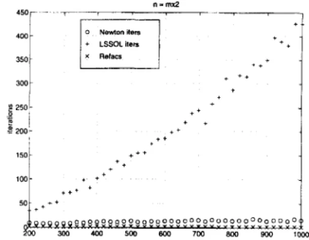
Fig. 2. Iteration results of the new method and LSSOL (n / nr = 2).

We compare the new method with the library routine LSSOL from Stanford University Systems Optimization Laboratory available in the NAG (1987) subroutine library. LSSOL contains implementations of a numerically stable active set strategy and the simplex method for the solution of linear and quadratic programs and least squares problems. It can also find a feasible solution to a system of linear inequalities by minimizing the sum of infeasibilities. Since it does not exploit sparsity of A, it makes a fair comparison to our method.

To illustrate the performances of the new method and LSSOL, we generated two sets of consistent systems of dense linear inequalities randomly. In the first set, we keep the ratio n/m constant at two and increase m from 100 to 500 in steps of 10. We

(9)

718 M.C. Pmar/European Journal of Operational Research IO7 (1998) 710-719 ___

_I

250 t 0 NwAcmilen i * Lsscxaers + + x Refacs ++ + + + ++ + A +

6

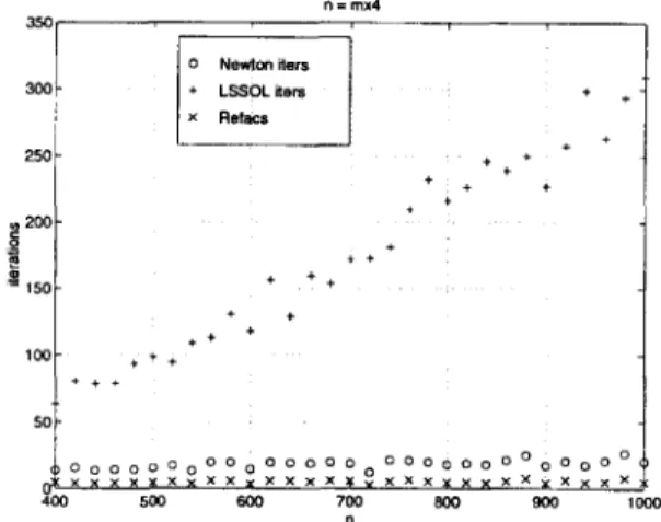
2co- 5 t e ??+ I _150- + ++ + + ++ + Ice- +++ ++r so-

Fig. 4. Iteration results of the new method and LSSOL (n/m = 4).

generate 10 problem instances for each pair (m,n) and solve these instances using the Newton method and LSSOL, respectively. This results in the solution of 410 problems by both methods. In the second set of problems, we keep the ratio n/m constant at four and vary m from 100 to 250 in steps of five. Hence, we solve 310 problems by both methods. In Figs.

l-4 we report the average statistics of these runs. In Figs. 1 and 3 we plot the average run time in CPU seconds while in Figs. 2 and 4 we plot the average number of iterations of the Newton method and LSSOL along with the number of refactorizations of A, AT in connection with the computations of the factors L and D.

The absolute level of infeasibility upon termination of the Newton algorithm is measured as the /Z-norm of the vector ( ATy - c>+ where t+=

max(O,t) and the plus operator is applied component- wise. This measure was found to be always less than or in the vicinity of 10 -13 in all test runs. These results demonstrate that the Newton algorithm is able to find an accurate feasible solution to linear inequalities efficiently. It attains a speed-up of three to four over LSSOL as the problem size is increased. This is a result of two factors:

1.

2.

The Newton method displays a slow growth rate in the number of iterations as the problems get larger.

The Newton method uses an almost constant number of refactorizations as the problem size is increased.

It seems that a sparse implementation of the Newton method will be a worthwhile research effort in the future.

Acknowledgements

The author is indebted to Kaj Madsen, Hans Bruun Nielsen, Wu Li and Bintong Chen for valu- able help. While this work was under review, we came across a recent reference Bramley and Win- nicka (1996) where an algorithm very similar to ours was independently proposed for the solution of linear inequalities. This algorithm is motivated from the theory of least squares and is apparently an extension of an unpublished work by Han (1980). A close inspection of these papers reveals that these authors use arguments different from ours in finite convergence proofs and they do not report computational comparisons with any other software. Their implementations also differ from ours. The author thanks R. Bramley for sending a copy of Han (1980).

References

Bramley, R., Winnicka, B., 1996. Solving linear inequalities in a least squares sense. SIAM Journal on Scientific Computing 17, 275-286.

Censor, Y., Zenios, S.A., 1997. Parallel Optimization: Theory, Algorithms and Applications. Oxford University Press, Ox- ford.

Chen, Ch., Mangasarian, O.L., 1995. Smoothing methods for convex inequalities and linear complementarity problems. Mathematical Programming 7 1, 5 l-69.

Clark, D.I., Osborne, M.R., 1986. Finite algorithms for Hub&s M-estimator. SIAM Journal on Scientific and Statistical Com- puting 7, 72-85.

Ekblom, H., 1988. A new algorithm for the Huber estimator in linear models. BIT 28, 123-132.

Fletcher, R., Powell, M.J.D., 1974. On the modification of LDLT factorizations. Mathematics of Computation 28, 1067-1087. Gentleman, W.M., 1973. Least squares computation by Givens

transformations without square roots. Journal of the Institute of Mathematics and its Applications 12, 329-336.

Gill, P.E., Hammarling, S.J., Murray, W., Saunders, M.A., Wright, M.H., 1986. User’s guide for LSSOL (Version 1.0): A Fortran package for constrained linear least squares and convex quadratic programming. Technical report SOL 86-l. Systems Optimization Laboratory, Department of Operations Research, Stanford University, Stanford, California.

(10)

Han, S-P., 1980. Least-squares solution of linear inequalities. Technical report TR-2141. Mathematics Research Center, Uni- versity of Wisconsin-Madison.

Herman, G.T., 1980. Image Reconstruction from Projections: The Fundamentals of Computerized Tomography. Academic Press, New York.

Hubcr, P.J., 1981. Robust Statistics. John Wiley, New York. Katznelson, S., 1965. An algorithm for solving nonlinear resistor

networks. Bell System Technical Journal 44, 1605-1620. De Leone, R., Mangasarian, O.L., 1987. Serial and parallel solu-

tion of large scale linear programs by augmented Lagrangian sucessive overrelaxation. In: Lecture Notes in Control and Information Sciences, Springer-Verlag.

Li, W., Swetits, J., 1993. A Newton method for convex regression, data smoothing, and quadratic programming with bounded constraints. SIAM Journal on Optimization 3, 466- 468.

Li, W., Swetits, 1997. A new algorithm for strictly convex quadratic programming. SIAM Journal on Optimization (to appear).

Li, W., 1997. Conjugate gradient algorithms for convex quadratic splines. Mathematical Programming (to appear).

Lin. Y., Pang, J.-S., 1987. Iterative methods for large convex quadratic programs: A survey. SIAM Journal on Control and Optimization 25, 383-411.

Luo, X.-D., Luo, Z.-Q., 1994. Extension of Hoffman’s error

bound to polynomial systems. SIAM Journal on Optimization 4, 383-392.

Madsen, K., Nielsen, H.B., 1990. Finite algorithms for robust linear regression. BIT 30, 682-699.

Mangasarian, O.L., 1981. Iterative solution of linear programs. SIAM Journal on Numerical Analysis 18, 606614.

Mangasarian, O.L., 1984. Normal solution of linear programs. Mathematical Programming Study 22, 206216.

NAG, 1987. Fortran library routine document. Numerical Analysis Group.

Nielsen, H.B., 1990. AAFAC: A package of Fortran 77 subpro- grams for solving ATAx = c. Report NI-90-11. Institute for Numerical Analysis, Technical University of Denmark. Rockafellar, R.T., 1987. Linear-quadratic programming and opti-

mal control. SIAM Journal on Control and Optimization 25, 781-814.

Rockafellar, R.T., 1990. Computational schemes for large-scale problems in extended linear-quadratic programming. Mathe- matical Programming, 447-474.

Rockafellar, R.T., 1976. Augmented Lagrangians and applications of the proximal point algorithm in convex programming. Mathematics of Operations Research 1, 97- 116.

Sun, J., 1992. On the structure of convex piecewise-quadratic functions. Journal of Optimization Theory and Applications 72, 499-5 10.