Selçuk J. Appl. Math. Selçuk Journal of Vol. 7. No.1. pp. 33-43, 2005 Applied Mathematics
Nonlinear Time Serıes Analysis Of Daily Gold Sale Price In Turkey ˙Ismail Kınacı and A¸sır Genç
Department of Statistics, Selcuk University, 42031 Konya, Turkey; e-mail: ikinaci@ selcuk.edu.tr, agenc@ selcuk.edu.tr
Received : March 16, 2005
Summary. A time series is a sequence of observations made periodically with a certain time interval. Since linear time series models are much more easier to make statistical inferences and forecasts, for modeling real life situations by a time series, a linear time series model should be considered first. However, in some cases, linear time series models can not properly explain the series and therefore a nonlinear model is inevitable. In this study, the series of daily gold sale prices between 2001 and 2004 in Turkey are used. For this series, a nonlinear and a linear best suited two model series are chosen, then their results are analyzed comparatively.
Key words: Linear Time Series Models, Nonlinear Time Series Models, La-grange Multiplayer Test
1. Introduction
Time series techniques are mostly used to estimate and forecast the time de-pendent data. Since the theory and applications of linear models are easy, these models are widely preferred. However, linear models can’t handle the following problems in data (Tong 1990).
The stationary solution of time series under linearity assumption approaches to a fixed point called “limit point” while time goes infinity. Therefore, the use of a linear model is hard for determining limit cycles.
Linear models can’t be appropriate for time irreversible data. Linear models aren’t suitable for the data with sudden jump points.
Because of above reasons, a nonlinear time series model might be needed in some cases. Kasap and Çelik (2004) used the self exciting threshold, autoregressive model for modeling the series of daily gold sale prices in Turkey.
2. Nonlinear Time Series Models
Linear time series models can be investigated in three main categories as Au-toregressive (AR), Moving Average(MA) or AuAu-toregressive Moving Average (ARMA) model which is a combination of AR and MA models. Since, AR and MA models are specific cases of ARMA model, in this study only ARMA model will be discussed as linear time series models. Here, ARMA models and some nonlinear time series models as Bilinear (BL), Smoothing Transition Autore-gressive (STAR), Threshold AutoreAutore-gressive (TAR), Exponential AutoreAutore-gressive (EAR) models will be investigated.
2.1. Threshold Autoregressive (TAR) Model
Threshold models have been firstly suggested by Tong and Lim (1980). Thanks to these models, a piecewise linear time series model can be used instead of non-linear time series models. One of threshold models is threshold autoregressive model in which each part is also an autoregressive model. Threshold models in th order can be expressed by,
(1) = ⎧ ⎪ ⎪ ⎨ ⎪ ⎪ ⎩ ()0 +()1 −1+ · · · + () −+()−1 (−1 −2 −) ∈ <() .. . ... ()0 +()1 −1+ · · · + () −+ () −1 (−1 −2 −) ∈ <() or (2) = ()0 + () 1 −1+· · ·+() −+()−1 (−1 −2 −) ∈ <()
and shortly shown by TAR(), where () ∼ ¡0 2¢ = 0 1 ,
()
are parameters of the model and <() is a partition of Euclidian space < and
called threshold region. 2.2. Bilinear (BL) Model
Bilinear models have been investigated by Grenger and Andersen (1978) in detail. Bilinear models can be expressed by
(3) = + X =1 −+ X =1 −+ X =1 X =1 −−+
and shortly shown by ( ). BL model is a linear model with respect to X or with respect to error term individually but a nonlinear model when these
are considered together. ( ) model is a specific case of BL model given by Eq.3 with = 0 and = 0.
2.3. Exponential Autoregressive (EAR) Model EAR(p,d) model is defined by,
(4) = + X =1 −+ £ exp¡−2−¢− 1¤ X =1 −+
Where −is transition variable, is delay parameter between 1 and and
is transition parameter.
2.4. Smoothing Transition Autoregressive (STAR) Model
The idea of smoothing transition was firstly introduced by Bacon and Watts (1971). ( ) model of order is defined as,
(5) = 1+ X =1 1−+ Ã 2+ X =1 2− ! (−− ; ) +
where (−− ; ) is continuous transition function, is transition
parame-ter, is delay parameparame-ter, − is transition variable and is middle point of
transition regime. If, (6) (−− ; ) = n 1 − exph− (−− )2 io
then ( ) model is transformed into exponential smoothing transition autoregressive (ESTAR) model (Tong 1990).
If the function (−− ; ∗) has logistic form
(7) (−− ; ∗) =
h
{1 + exp [−∗(−− ∗)]}−1− 05
i
then model is transformed into logistic smoothing transition autoregres-sive (LSTAR) model.
2.5. Autoregressive Conditional Heteroscedastic (ARCH) models
The model was firstly introduced by Engle (1982). The ( )model is in () form
(8) = +
X
=1
−+
Except that the term is defined by
(9) = p where (10) = 0+ X =1 2−
Thus, this is the source of nonlinearity. For the positive values of , we must
have 0 0 {}=1> 0. Furthermore, the sum of = 1 2 must
be greater than 1 for stationarity (Zhang, 2002).
3. Linearity Test: Lagrange Multiplier (LM) Test
Whether a time series has a nonlinear structure or not, can be tested by La-grange Multiplier test. This test differs from others in the sense that a linear model is tested against a nonlinear model. Therefore, it is necessary to describe an ARMA model for the series to perform LM test. ARMA models are known as Box-Jenkins models and clearly investigated by Box at all (1994). The LM test can be constituted for almost all nonlinear time series alternatives. The hypothesis for LM test is,
(11) 0: ” ” 1: ” ”
Here the LM test steps can be performed by only estimating the linear model given in null hypothesis. This means that a LM test constructed for only one alternative will be valid for various alternatives.
The LM test statistics for testing the hypothesis given in (11) is defined as,
(12) = ˆ2 Ã X =1 ˆ 1 !0³ ˆ 11− ˆ12ˆ22−1ˆ21 ´−1ÃX =1 ˆ 1 !
The LM test statistics will have chi-square distribution of order under the null hypothesis. Here, is the number of parameters restricted under the null hypothesis (Saikkonen and Luukkonen 1988, Subba Rao and Gabr 1980, Zhang 2002).
4. Application
In this study, the series of daily gold sale prices (TL/gr) taken form Central Bank of The Republic of Turkey between 23.02.2001 and 07.07.2004 will be used. Firstly, the most appropriate linear time series model will be deter-mined among the ( ), = 0 1 5 = 0 1 5 models ac-cording to AIC criterion and then this model will be compared with each of ( ) ( ) ( ), ( ) and ( ) by using LM test. In the last step of the application, forecasting values of chosen two models from the linear and the nonlinear models will be given.
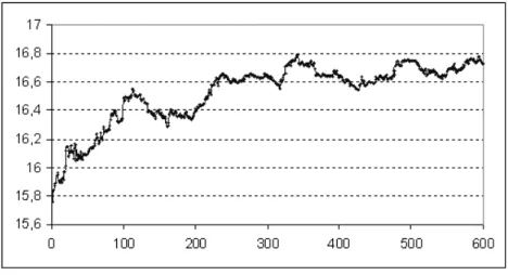
In this study, natural logarithmic transformation is applied to the series and it is called “ln-golden”. The time series plot of ln-golden series is given in Fig.1.
Figure 1. Ln-golden series
We can obviously observe from Fig.1 that the average of the ln-golden series fluctuates in time. This means that the average of the series is time dependent. This case shows that the ln-golden series is nonstationary. Because, the average and the variance of a stationary time series are not dependent on time. In order to satisfy stationarity of ln-golden series, first order difference operator has been applied to the ln-golden series and a new series has been obtained. The time series plot of this new series is given in Fig.2.
Figure 2. Differenced ln-golden series
According to Fig.2, the average of the differenced ln-golden series doesn’t change with the time. This case indicates that the new series is stationary.
4.1. Determination of Linear Model
First, we will investigate the most appropriate linear time series model for the differenced ln-golden series. As mentioned before, we can use the AIC criterion to choose the most appropriate model among the estimated models. Here, appropriate linear time series model has been selected among the ( ) with = 0 1 5 = 0 1 5 according to AIC criterion and it has shown that the most appropriate model for the differenced ln-golden series is AR(1) model. The estimation results of AR(1) model and the value of Augmented Dickey Fuller (ADF) test statistics for AR(1) model are given in Table 1.
Parameters Estimated values Standard Errors t-value p-value
0 0.0018 0.0008 2.28 0.023
1 -0.1407 0.0405 -3.47 0.001
SSE = 0.230 , MSE = 0.00038 , AIC = -5.03 -28.16 , Critical value = -1.94 Table 1. Estimation results for AR(1) model
As shown by Table 1, the value of ADF test statistics computed for AR(1) model is less than the critical value for = 005 significance level, that is, AR(1) model is stationary. Furthermore, all parameters in AR(1) model are statistically significant, because all of the p-values obtained for parameters in AR(1) model are less than = 005 significance level.
Predicted and observed values of ln-golden series using AR(1) model are shown in Fig.3.
Figure 3. Observed and forecasted values of ln-golden series
In addition, forecasting values for ln-golden series using AR(1) model described for differenced ln-golden series are given by Fig.4.
Figure 4. Forecasted values obtained by AR(1) model
From Fig.4, forecasting values approaches to the average value 0.0016. This indicates that AR(1) model for the differenced ln-golden series is stationary. As a result, three important points should be noted that AR(1) model for the differenced ln-golden series has minimum AIC value among all of the estimated models, its parameters are statistically significant and its residuals have white noise processes. Therefore, we concluded that AR(1) model is an appropriate and a significant model for the differenced ln-golden series. But it shouldn’t be overlooked that AR(1) model is appropriate model only among linear time series
models. In the next step of application, we will try to answer the question “can we describe a nonlinear model which has better performance than AR(1)?”. 4.2. Determination of Nonlinear Time Series Model
Before determining a nonlinear model for the differenced ln-golden series, it is useful to test AR(1) model against some nonlinear time series models as BL, ESTAR, EAR, LSTAR and ARCH. If a nonlinear model is accepted by using any linearity test then this model can be estimated.
4.2.1. Results of Lagrange Multiplier (LM) Test
As mentioned in section 3, LM test can be used to test a linear model against any nonlinear time series model. Here, AR(1) model has been tested against nonlinear alternatives as , and , and it has shown that AR(1) model is rejected only against ARCH model. The LM test results used for testing AR(1) model against ARCH model are given in Table 2.
2 095; Decision 1 30.916 3.841 ARCH(1,1) 2 34.125 5.991 ARCH(1,2) 3 36.379 7.815 ARCH(1,3) 4 36.506 9.488 ARCH(1,4)
Table 2. LM test results for(1)model against(1 )
In Table 2, since the values of LM test statistics computed for = 1 2 3 4 are greater than the values of 2095; ,(1) model is rejected against (1 ) models for = 1 2 3 4, that is, there is effect in ln-golden series. In this case, it is tried to determine a model which can remove the ARCH effect in ln-golden series and it is found that the most suitable one is,
= 0+ 1−1+ − 1−1 (13)
=
q
0+ 12−1
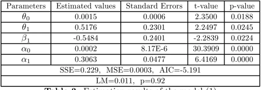
Parameter estimation results of this model and the value of LM test statistics for the presence of the ARCH effect are given in Table 3.
Parameters Estimated values Standard Errors t-value p-value
0 0.0015 0.0006 2.3500 0.0188
1 0.5176 0.2301 2.2497 0.0245
1 -0.5484 0.2401 -2.2839 0.0224
0 0.0002 8.17E-6 30.3909 0.0000
1 0.3063 0.0477 6.4169 0.0000
SSE=0.229, MSE=0.0003, AIC=-5.191 LM=0.011, p=0.92
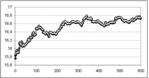
According to the results given in Table 3, all parameters in the model are statis-tically significant. In addition, the LM test results show that the ARCH effect is removed. Prediction values for ln-golden series by model (1) and observed values are shown in Fig.5.
Figure 5. Observed and predicted values
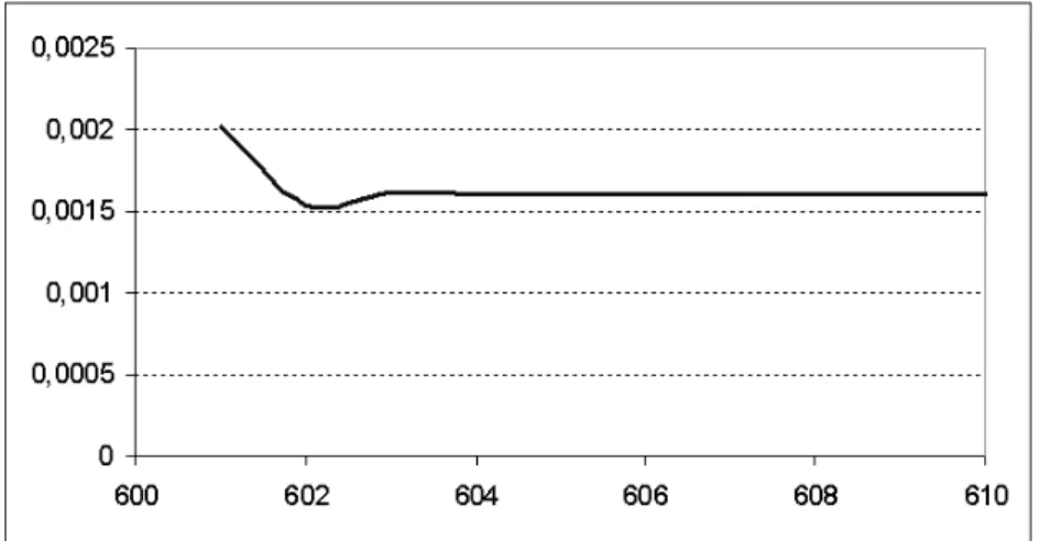
Fig.6. indicates the forecasting values for the differenced ln-golden series.
Figure 6. Forecasting values for differenced ln-golden series The autocorrelation function of the residuals of model (1) is shown in Fig.7.
Figure 7. Autocorrelation functions of model residuals
From Fig.7, since all autocorrelation coefficients are within the confidence band, it can be concluded that the residuals have white noise processes.
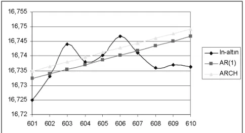
In the last step of application, the forecasting values for ln-golden series obtained by using AR(1) and (13) models are shown in Fig.8.
Figure 8. Forecasting values for ln-golden series
5. Results
In this study, the series of daily gold sale price (TL/gr) between 23.02.2001 and 07.07.2004 in Turkey are used. The AR(1) model is determined for the differenced ln-golden series to be a linear time series model and this model has been tested against nonlinear alternatives as , and , and it has been shown that AR(1) model is rejected only against ARCH model. In this case, it is tried to determine a model which can remove the ARCH effect in ln-golden series and it is found that the most appropriate model is,
(14) = 0+ 1−1+ − 1−1 =
q
0+ 12−1
Since there is no ARCH effect in model (13), the results of this model seems to be more reliable than those of AR(1).
References
1. G. E. Box, G. M. Jenkins, G.C. Reinsel (1994): Time Series Analysis: Forecasting and Control, Holden-Day, San Fransisco.
2. C. Granger, A. Anderson (1978): Introduction to Bilinear Time Series Models, Vandenhoeck and Ruprect, Göttingen.
3. R. Kasap, N. Çelik (2004): Kendinden uyarımlı e¸siksel otoregressif (SETAR) model ve altın fiyatları üzerine uygulaması, GÜ ˙I˙IBF Dergisi.
4. ˙I. Kınacı(2005): Nonlinear time series models, Doctora thesis, Selçuk University, Konya
5. P. Saikkonen, R. Luukkonen (1988): Lagrange Multiplier Test for Testing Non-linearities in Time Series Models, Scandinavian Journal of Statistics, 15: 55-68. 6. T. Subba Rao, M. Gabr (1980): A Test for Linearity of Stationary Time Series, Journal of Time Series Analysis, 1: 145-152.
7. H. Tong (1990): Non-linear Time Series: A Dynamical System Approach, New York, Oxford University Press.
8 H. STong, K. Lim (1980): Threshold Autoregression, Limit Cycles and Cyclical Data, Journal of the Royal Statistical Society, B42: 245-292.
9. Y. Zhang (2002): Testing for nonlinearities in time series with an application to exchange rates, Doctora thesis, Iowa State University, Iowa.