I
ACKNOWLEDGEMENTS
Foremost, I would like to express my sincere gratitude to my supervisor Doç. Dr. Emine MEŞE and I want to say thank to Y.Doç. Dr. Ahmet BİNGÜL for the continuous support of my M.Sc. Study and research, for their patience, motivation, enthusiasm and immense knowledge. Their guidance helped me in all the time of research and writing of this thesis. I could not have imagined having a better advisor and mentor M.Sc. study.
Meanwhile, I want to say thank to Mehmet ARSLAN and Özgür ÖZTEMEL for their help and I want to say thank to Emrah ŞAHİN for his help and for helping me to motivate on my M.Sc. Study.
II CONTENT Page ACKNOWLEDGEMENTS……….... I CONTENT……… II ABSTRACT……….. IIV LIST OF TABLES………... V LIST OF FIGURES………. VI
LIST OF SYMBOLS………... VIII
CHAPTER 1 INTRODUCTION 1.1 Introduction ………..……. 1 CHAPTER 2 CP VIOLATION 2.1 Parity Transformation………..… 3 2.2 Charge Conjugation……….…………. 5
2.3 Charge Conjugation and Parity………...…….………... 7
2.4 CP Violation and The Standard Model Lagrangian 8 2.5 The CKM Matrix ………... 9
CHAPTER 3 CP VIOLATION IN NEUTRAL KAON SYSTEM 3.1 CP and Pion………... 13
3.2 The NeutraL Kaon System……….…….. 14
3.3 Discovery Of CP Violation in The Kaon System ………. 17
3.4 Regeneration ………... 19
III CHAPTER 4
THE LARGE HADRON COLLİDER (LHC)
4.1 The Large Hadron Collider (LHC) ………. 23
4.1.1 The Cern Accelerator Complex ………... 25
4.2 The Atlas Detector……….... 26
4.2.1 The Atlas Coordinate System……….………..……. 28
4.2.2 Inner Detector…………..….……….. 28
4.2.3 Calorimeter……….. 31
4.2.4 Muon Spectrometer………... 35
4.2.4.1 The toroidal magnets………... 36
4.2.4.2 Muon chamber types……….………... 37
CHAPTER 5 DATA ANALYSIS AND RESULTS 5.1 Overwiew 39 5.2 Photon Reconstruction …….………... 43
5.3 Choosing Photon From Caloclusters………... 49
5.4 Pion Reconstruction……….………….. 50
5.5 Kaon Reconstruction……… 63
CONCLUSION………. 67
IV
ABSTRACT
CP VIOLATION IN THE NEUTRAL KAON SYSTEM MSc THESIS
Selim ASLAN UNIVERSITY OF DICLE
INSTITUTE OF NATURAL AND APPLIED SCIENCES DEPARTMENT OF PHYSICS
2013
As we know there are some symmetries in the universe, but now we all know that the universe are formed by symmetries violation. The most important violation of symmetry is CP (charge-parity) violation. Scientists had discovered CP violation in the neutral kaon nearly 50 years ago. But today scientists need to study on this topic because the scientists want to learn more information about CP violation.
In this thesis, we will try to examine some basic information of CP violation and neutral Kaon and We will analysis the Atlas data if We can see CP violation in the neutral Kaon system.
V
LIST OF TABLES
Table 4.1. Some basic parameters of the LHC at design luminosity 23 Table 4.2. General performance goals of the ATLAS detector. 27 Table 4.3. Main parameters of the ATLAS inner-detector system. 30 Table 4.4. Main parameter of the ATLAS calorimeter system. 32
Table 4.5. The main parameters of the muon chambers 36
Table 5.1 Atlas data parameters 40
VI
LIST OF FIGURES
Figure 2.1 Mirror reflection of axial vectors 3
Figure 2.2 The Cabibbo angle 10
Figure 3.1 Sketch of the apparatus of Christenson, Cronin, Fitch, and Turlay at Brookhaven (Christenson et al., 1964). The cross-hatched area is the fiducial region for decays.
21
Figure 3.2 (a) The measured two “pion” mass spectrum. (b) The distribution of the cosine of the angle between the summed momentum vector of the two pions and the direction of the beam. (c-e) The angular distribution for different ranges in the invariant mass
22
Figure 4.1 Schematic layout of the LHC 24
Figure 4.2 CERN accelerator complex 25
Figure 4.3 Cut-away view of the ATLAS detector. 26
Figure 4.4 Cut-away view of the ATLAS inner detector. 29
Figure 4.5 Cut-away view of the ATLAS calorimeter system. 32
Figure 4.6 Cut-away view of the ATLAS muon spectrometer. 36
Figure 5.1 value distribution of photons reconstructed from electron and positron pairs for conversions vector
44
Figure 5.2 Eta (η) value distribution of photon reconstructed form electron and positron pairs for conversions vector
45
Figure 5.3 q/p value distribution of photon reconstructed from electron and positron pairs for conversions vector
46
Figure 5.4 Momentum distribution of photon reconstructed from electron-positron pairs from conversions vector
47
Figure 5.5 Energy distribution of photons which are reconstructed from electron-positron pairs from conversions vector
48
Figure 5.6 the energy distribution of photons reconstructed from electron-positron pairs on the space
51
Figure 5.7 the distribution of weta1 for choosing photons 52 Figure 5.8 the distribution of e2tsts1 for choosing photons
Figure 5.9 the distribution of ethad1for choosing photons
53 54
VII
Figure 5.10 the distribution of emins1 for choosing photons Figure 5.11 the distribution of emaxs1 for choosing photons Figure 5.12 the distribution of wtots1 for choosing photons Figure 5.13 the distribution of wtots1 for choosing photons Figure 5.14 the distribution of f1 for choosing photons
55 56 57 58 59 Figure 5.15 the distribution of pion invariant mass
Figure 5.16 the distribution of pion invariant mass
60 61 Figure 5.17 the distribution of kaon invariant mass
Figure 5.18 the distribution of kaon invariant mass Figure 5.19 the distribution of kaon invariant mass Figure 5.20 the distribution of kaon invariant mass
63 64 64 65
VIII Neutral Kaon Longlife Kaon Shortlife Kaon Pion P Parity L Angular momentum C Charge conjugation Proton Sigma Muon Muon neutrino Electron Electron neutrino Charge Baryon number ᴧ Lambda Neutron α Eigenvalue J Charge density
Electromagnetic vector potential
Photon S Strangeness
CDF The Collider Detector at Fermilab ~4 t.f. Four times finner
Etc. Et cetera A Ion
CERN The European Organization for Nuclear Research LHC The Large Hadron Collider
ATLAS A Toroidal LHC Apparatus ALICE A Large Ion Collider Experiment CMS Compact Muon Selenoid
IX
LCHb Large Hadron Collider beauty Experiment Linac Linear accelerator
PSB Proton Synchrotron Booster PS Proton Synchrotron
SPS Super Proton Synchrotron AD Antiproton Decelerator ISOLDE Online Isotope Mass Separator CNGS CERN Neutrinos to Gran Sasso nTOF Neutron tome-of-flight facility ID Inner Detector
SCT Semi-Conductor Tracker TRT Transition Radiation Tracker EM Electromagnetic Calorimeter
EMEC Electromagnetic end-cap Calorimeter HEC Hadronic end-cap Calorimeter FCal Forward Calorimeter
MDT’s Monitored Drift Tubes CSC’s Cathode Strip Chambers RPC’s Resistive Plate Chambers TGC’s Thin Gap Chambers mc Montecarlos Data da Real Data
1 CHAPTER 1
INTRODUCTION 1.1 Introduction
Symmetries play very important role in physics. They often simplify the analysis of complex systems. These symmetries may be continuous or discrete. There is a corresponding conservation law for each symmetry. In the real physical world, some of the symmetries are exact and some are broken. The studies of symmetries conserved as well as broken ones are all important. These studies have provided many insights for the understanding of the fundamental principles of the universe. Different interactions in nature have different symmetry properties.
Discrete symmetries like C (charge conjugation) and P (parity or space reflection) have played a very important role in the understanding of elementary particle interaction. C and P are conserved in strong and electromagnetic processes, but violated in weak decays. For several years it was believed that the product CP was conserved in all kinds of interactions. However, in 1964 Christenson, Cronin, Fitch and Turlay showed for the first time through their famous experiment in the neutral kaon decays that CP, like parity, was also not a good symmetry of nature. (Christenson et al. t1964) (Sozzi 2008) This surprising effect is a manifestation of indirect CP violation. The mass eigenstates of the neutral kaon system are the admixture of the flavour eigenstates and ̅̅̅̅. The CP violation occurs due to the fact that are not eigenstates of the CP operator. In particular, the state is
governed by the CP-odd eigenstate, but also has a tiny admixture of the CP even eigenstate, which may decay through CP-conserving interactions into the final state.
The main purpose of this thesis is to investigate CP violation in the neutral Kaon system since CP violation is very important in particle physics. It gives us the chance of understanding the universe, interaction between matter and antimatter and more importantly it makes easier for us to understand the basic information of the Big-Bang.
INTRODUCTION
2
In this thesis, at first in chapte 2 some basic information about CP violation like parity and charge conjugation and Cabibbo-Kobayashi-Maskawa matrix which is important for understanting fundamental of CP violation will be introduced. Then, theory of CP violation in neutral Kaon system will be given in chapter 3. In chapter 4, we will introduced the experimental set up of Large Hadron Collider and one of its main part, Atlas detector, where data used for CP violation in thesis is produced. This data provided by Yr. Doç. Dr. Ahmet BİNGÜL who is a staff in the University of Gaziantep and also a member of Atlas. The analysis of data will be given in chapter 5. The provided data consist of many vectors such as MonteCarlos, Tracks, Conversions and Calocluster. The data is analyzed with Root which provides a set of object-oriental frameworks needed to handle and analyze large amounts of data in a very efficient way.
3 CHAPTER 2
CP VIOLATION
2.1 Parity Transformation
(Sozzi 2008)Parity is an operator that takes us from a right handed coordinate frame to a left handed one, (or vice versa). This operator is also called space inversion operator.
Figure 2.1 Mirror reflection of axial vectors
Under parity transformation (P) the space-time four-vector changes as follows: ( ) → ( )
CP VIOLATION
4
Consider a scalar wavefunction Performing the parity operation on this wavefunction will transform it to
Until 1956 the general feeling was that all physical processes would conserve parity. In this year, however, a number of experiments were performed which showed that at least for processes involving the weak interaction this was not the case.
Spin like angular momentum transforms as the cross product of a space vector and a momentum vector (Bigi and Sanda 2009).
⃗ ⃗⃗ , ,
And so
⃗ ⃗
In other words the parity operation leaves the direction of the spin unchanged. If one can thus find a process which produces an asymmetric distribution with respect to the spin direction one proves that P-symmetry is not conserved.
Another way of looking at it is by considering helicity which is the projection of the spin of a particle onto its direction of motion,
̂ (2.1)
As helicity changes sign under parity transformation if we find a process which produces a particle with a preferred helicity also proves that P-symmetry is violated.
5 2.2 Charge Conjugation
(McMahon 2008) We now consider charge conjugation C, an operator which converts particles into antiparticles. Let ǀ 〉 represent a particle state and 〉 represent the antiparticle state. Then the charge conjugation operator acts as
〉 〉
If we apply the charge conjugation operator on an antiparticle, it will transform antiparticle to particle as
̅ 〉 〉
By applying C operator on a particle again we get this 〉 〉 | 〉 〉
We can use this relation to determine the eigenvalues of charge conjugation. Eigenvalue of like the eigenvalue of P. As charge conjugation converts particles into antiparticles and vice versa, it reverses the sign of all quantum numbers. Consider a proton 〉. It has positive charge
〉 〉
where is any operator chosen to calculate the eigenvalue of C operator.
and Baryon number . Apply the charge conjugation operator on the proton 〉 〉
and
〉 〉
CP VIOLATION
6
Notice that the proton state cannot be an eigenstate of charge conjugation, since the result of 〉 〉 is a state with different quantum numbers, α, and different quantum state. The eigenstates of the charge conjugation operator are eigenstates with 0 charge. For example we can look at the neutral pion . In this case, is its own antiparticle and so
〉 〉
Applying charge conjugation twice
〉 〉 〉
(2.2)
We can find the charge conjugation properties of the photon in the following way, and determine the eigenvalue α for the . First charge conjugation will reverse the sign of the charge density J as shown.
(2.3)
Now, the interaction part of the electromagnetic Lagrangian can be used to determine the charge conjugation properties of the photon. The action of on gives
. (2.4)
This can only be invariant if
7
Where is the electromagnetic vector potential, therefor the eigenvalue of charge conjugation for the photon is obtained to be ⟨ .Therefore if there are n photons, the charge conjugation is . The decays into two photons as
The two photon state has , therefore it is concluded that ⟩ ⟩
for the
This demonstrates that charge conjugation C is conserved in the strong and electromagnetic interactions but not in the weak interaction.
2.3 Charge Conjugation and Parity (CP)
(Burcham 1973) The fact that charge conjugation and parity are each individually violated in weak interactions led to the hope that the combination of charge conjugation and parity would be conserved in weak interactions. The weak interactions are almost invariant under the combined operations of charge conjugation and parity inversion, this process is known as “CP”.
The weak interactions allows a (highly relativistic) left-handed (negative helicity) electron to convert into a neutrino emitting a or alternatively a decays into a left-handed electron and an antineutrino. Similarly a right-handed (positive helicity) positron to convert into an antineutrino. If it were possible to repeat the experiment of Chien-Shiung Wu using the antiparticle of 60Co, 60Co which decays into 60Ni emitting positrons and neutrinos, one would find that the positrons tended to be emitted in the same direction as the spin of the antinucleus. however in the original experiment they tended to be emitted in the opposite direction from the spin of the nucleus.
CP VIOLATION
8
2.4 CP Violation and The Standardmodel Lagrangian
(Kooijman and Tuning 2011) CP violation shows up in the complex Yukawa couplings. We examine the Yukawa part of the Lagrangian
̅̅̅̅
̅̅̅̅ ̅̅̅̅̅ (2.6)
Where complex matrices, is the Higgs field, and are generation labels and is the dynamics of the spinor fields.
The CP operation transforms the spinor fields as follows ( ̅̅̅̅ ) ̅̅̅̅̅
So, remains unchanged under the CP operation if = .
Similarly, at the charged current coupling in the basis of quark mass eigenstates is
√ ̅̅̅̅ √ ̅̅̅̅ . (2.7)
where is left-handed quark doublets, are elements of cabibbo-kobayashi-maskawa matrix, and are right-handed down- and up-type quark singlets, respectively. The CP-transformed expression given equation 2.7 as follows
√ ̅̅̅̅ √ ̅̅̅̅
9
The Lagrangian is unchanged. If the elements of the CKM matrix provides the equality of = .
The complex nature of the CKM matrix is the origin of CP violation in the Standard Model.
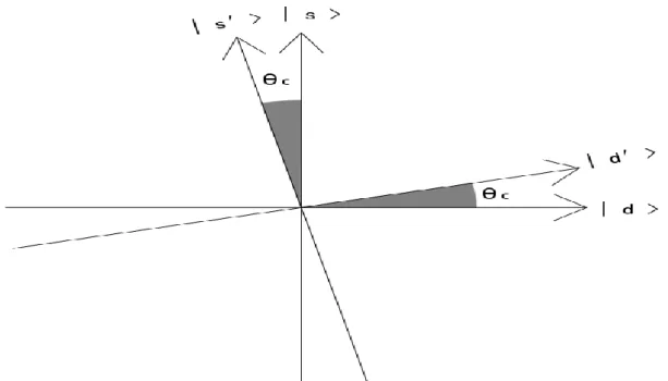
2.5 The CKM Matrix
The Cabibbo–Kobayashi–Maskawa matrix is a unitary matrix which contains information on the strength of flavour-changing weak decays. One can specify the mismatch of quantum states of quarks when they emit freely and when they take part in the weak interactions. Therefore CKM matrix has a very important role for understanding of CP violation..
The CKM mixing matrix can be parametrized in many equivalent ways by choosing the angles.
( ) ( )
where and is the CP-violating phase. Each angle
is here labelled with the indexes corresponding to the mixing of two families, so that
would indicate that families and are decoupled; all these angles can
always be chosen to lie in the first quadrant (Wolfensteien 1983).
Using the currently accepted values for and , the Cabbibo angle can be
calculated
CP VIOLATION
10
Figure 2.2 The Cabibbo angle
The Cabibbo angle represents the rotation of the mass eigenstate vector space formed by the mass eigenstates into the weak eigenstate vector formed by the weak eigenstate .
and
This can be written in matrix notation as follows
[ ] [
] [ ]
Or we can write by using the Cabbibo angle
[ ] [ ] [ ]
where the various represent the probability that the quark of flavor decays into a quark of flavor. This 2 × 2 rotation matrix is called the Cabibbo matrix. Observing that CP-violation could not be explained in a four-quark model,
11
Kobayashi and Maskawa generalized the Cabbibo matrix into the Cabibbo– Kobayashi–Maskawa matrix (or CKM matrix) to keep track of the weak decays of three generations of quarks
[ ] [
] [ ] .
On the left is the weak interaction doublet partners of up-type quarks, and on the right is the CKM matrix along with a vector of mass eigenstates of down-type quarks. The CKM matrix describes the probability of a transition from one quark i to another quark j. These transitions are proportional to (Ceccucci et al. 2008).
Currently, the best determination of the magnitudes of the CKM matrix elements is
[ ] [ ] [ ]
CP VIOLATION
13 CHAPTER 3
CP VIOLATION IN NEUTRAL KAON SYSTEM
3.1 CP and Pion
(Bigi and Sanda 2009). The is a pseudoscalar meson consisting of a quark and an antiquark. The total wave function of the must be symmetric as it has spin 0. It must however be antisymmetric under the interchange of the spin of quark and anti-quark as these are fermions. Therefore the wave function must also be antisymmetric under interchange of the positions of the quark and antiquark.
〉 ̅ 〉 ̅ 〉 ̅ 〉 ̅ 〉.
Performing parity transformation then yields
〉 ̅ 〉 ̅ 〉 ̅ 〉 ̅ 〉 〉.
The is thus an eigenstate of the Parity operation with eigenvalue -1.
Performing the C-operation
〉 〉 .
This can also be deduced from the fact that it decays into two photons. A photon is nothing more than a combination of electric and magnetic fields and the C operation will invert both components. That is
CP VIOLATION IN NEUTRAL KAON SYSTEM
14 from which it follows that
〉 〉 〉 〉 The combined transformation
〉 〉 . (3.1)
and thus, it is a CP eigenstate with eigenvalue -1.
(McMahon 2008) The system 〉 must be symmetric under interchange of the two particles as they are identical bosons. The CP operation will therefore be merely the product of the CP operation on the two s separately
〉 〉 〉 .
For the 〉 system the C operation interchanges and and the P operation changes them back again so that the full CP operation is equivalent to the identity transformation:
〉 〉 〉 .
All systems of two pions are eigenstates of CP with eigenvalue . They are thus “CP-even”. All systems of three pions are eigenstates of CP with eigenvalue 1. The 〉 system is again simple because we are dealing with identical bosons the CP operation is the product of the operation on the three pions separately
〉 〉 〉
It is therefore a CP-odd system.
3.2 The Neutral Kaon System
(Das and Ferbel 2005) Considering the neutral components of mesons, ( ) and ̅̅̅ ̅ form particle and antiparticle counterparts with strangeness and −1, respectively. In comparison, neutron and anti-neutron are also neutral with
15
baryon number = 1 and −1. However, those two are completely different since baryon number is a rigidly conserved number while is only conserved in strong interaction and electromagnetic interaction. In a weak process, a decay mode with can exist.
̅̅̅
The reverse process of the second one: ̅̅̅ is also possible. Thus, mixing can occur via virtual intermediate states,
̅̅̅
From the above discussion we can see particle and anti-particle can mix via weak interaction, however, no mixing will occur between neutron and anti-neutron since is rigidly conserved. The transition from to ̅̅̅ has and thus it is a second-order weak interaction. It implies a pure state at and it will become a superposition of and ̅̅̅ at a later time t.
Assume the decay amplitude of is then the decay amplitude of ̅̅̅ is according to theorem. Define the following linear combination:
〉 √ 〉 ̅ 〉 〉 √ 〉 ̅ 〉 (3.2) (3.3)
(Sozzi 2008) Thus the decay amplitudes of and are √ and 0, respectively. Since is the easiest decay mode of meson, Eqns. (3.2) and (4.3) imply has a long life-time while has a short life-time, and decays via other channels (mainly through ). With a smaller phase space compared with mode, the life-time of is thus longer. We can take and , thus
CP VIOLATION IN NEUTRAL KAON SYSTEM 16 〉 √ 〉 ̅ 〉 〉 √ 〉 ̅ 〉 (3.4) (3.5)
and are two different states. They have definite life-time, but
uncertain value (since is not conserved in weak interaction). In comparison, and ̅̅̅ are states generated through strong process.
Following experiments which is based on this physical picture can be done. Considering the generation of through scattering:
From Eqn. (3.4) and (3.5), we have
√ 〉 〉 (3.6)
Where component will disappear due to decaying into and component is left. Notice from Eqn. (3.5) that is the equal-amount mixing of and ̅ , a portion of has been converted into ̅ to test the existence of ̅ , we can check via the following interaction:
̅ {
Since cannot be generated from (strangeness number for and
are and 1, respectively, if or ( ) can be detected, ̅ can thus be verified to exist in the beam. Experiments have shown, after going through the second slab, ̅ is absorbed and is left to continue propagation. This process is called regeneration (will be given in 3.4 in more detail).
17
3.3 Discovery of CP Violation in Kaon System
(Bigi and Sanda 2009) The discovery of parity violation at the end of the 1950’s was already a surprise. However, once such an assumption had been shown once to be invalid, it was natural to see if other symmetries were broken. Applying the CP operator on neutral kaon
〉 ̅ 〉 and
̅ 〉 〉.
Here ̅ 〉 and ̅ 〉 states are not the eigenstates of CP, because the wave function is changed by this operation from one to the other. We can construct these eigenstates like that.
〉
√ 〉 ̅ 〉 and
〉
√ 〉 ̅ 〉 .
Now, the states 〉 and 〉 are the CP eigenstates.
〉 〉 and
〉 〉.
If CP is conserved, the state 〉 will only decay into (or with a higher angular momentum to ) whereas the the state 〉 is strictly forbidden to decay into a two pion final state. Because the mass of the is approximately 497.6 MeV and the mass of a pion is about 139.6 MeV the available phase space for the two pion decay is almost a factor of 1000 larger than that available for the three pion decay. As a result, the lifetime of the CP-odd eigenstate of the -system is very large, much larger than the lifetime of the CP-even
CP VIOLATION IN NEUTRAL KAON SYSTEM
18
eigenstate. This is the reason that the CP-eigenstates are referred to as the and , where the subscripts stand for short and long, respectively, and not referred to as heavy and light as is done in the -system,
〉
√ 〉 ̅ 〉 and
〉 √ 〉 ̅ 〉 .
Now by applying CP on and
〉 ( √ 〉 ̅ 〉 ) (√ ̅ 〉 〉 ) √ 〉 ̅ 〉 〉 ( √ 〉 ̅ 〉 ) (√ 〉 ̅ 〉 ) ( √ 〉 ̅ 〉 ) Namely; 〉 〉 〉 〉
Asuming CP is conserved in the weak interactions then 〉 can only decay into a state with and 〉 can only decay into a state with
Neutral kaons decay into two or three pions. But we have already known that two pions system carries a parity of +1 and three pions system carries a parity of -1 but both have . So may decays into two pions and decays into three pions.
19 3.4 Regeneration
(Kooijman and Tuning 2011) Here we will discuss the effects of the passage through matter of a state which is a superposition of 〉 and ̅ 〉. In the Hamiltonian we will now also have to take into account the strong interactions of the state with the matter it is passing through. We will neglect any inelastic interactions as these will merely decrease the intensity. We know from experiment that the strong interactions of 〉 and ̅ 〉 are different. The ̅ 〉 ( ̅) contains an s-quark and can produce strange baryon resonances, like
̅ 〉
So the total cross section for scattering will be smaller than for ̅ .
Suppose that a pure beam would incident on matter where all ̅ would be absorbed, then the outgoing beam would be pure . Similar to a Stern-Gerlach filter, half of the outgoing kaons would then decay as a and half as .
√ 〉 〉
In principle the effect seen in the Cronin experiment could have been due to regeneration of the beam. If this would be the case then clearly by introducing more material in the path of the beam the effect would increase. The experiment was therefore repeated with liquid hydrogen instead of He (helyum) in the decay path. The density and so the size of the regeneration then grows by a factor of 1000. The growth of the signal was found to be the equivalent of 10 events. The experiment was also repeated with the He replaced by vacuum. The signal persisted, so that regeneration could be ruled out as the cause.
Finally, one has to prove that the particle which decays into the state is in fact the state. To prove this one determined that there existed interference between the state decaying into and a regenerated .
CP VIOLATION IN NEUTRAL KAON SYSTEM
20
The only remaining conclusion was therefore that CP-symmetry is violated in weak interactions.
3.5 The Cronin-FITCH Experiment
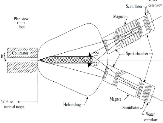
(Christenson et al. 1964) Until 1964 all measurements were consistent with the notion of CP-symmetry, even those which involve the weak interaction. In fact CP-symmetry was invoked to explain the large difference in lifetime between the and . The experiment which unexpectedly changed this situation was performed by Christensen, Cronin, Fitch and Turlay in 1964.
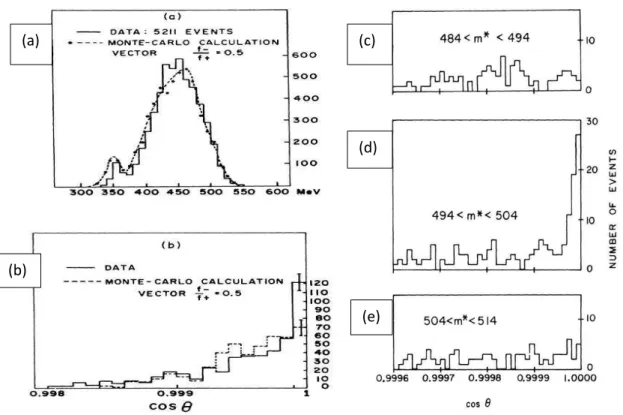
The experimental layout is shown in Figure 3.1. It consisted of a Be-target placed in a beam. All particles produced in the interactions, including any were allowed to decay in a low pressure He-tank. Decay products were detected in two magnetic spectrometers placed roughly 20 m from the target. The distance of 20m corresponds to approximately 300 lifetimes for the . All decay products must therefore come from the . All opposite charge combinations of particles, which had a reconstructed decay vertex within the He-volume were analysed and their invariant mass was determined under the assumption that both detected particles were pions. Obviously one expects to observe invariant mass combinations with a mass smaller than the mass emanating from the decay ( )). However some background was produced in the experiment from the decays and where the and the are misidentified as pions. Figure 3.2a shows the measured spectrum. The figure shows a Montecarlo prediction from all known decays of the (e.g. the peak at about 350 MeV is from the decay. At first
21
Figure 3.1: The experimental apparatus with which CP violation was first measured
glance there is no real discrepancy between the measurements and the MC prediction. Certainly there is no indication of an excess of events at around 500 MeV. If they however plot the cosine of the angle between the flight path of the and the direction of the momentum sum of the two particles for 490 < < 510 MeV we start to see an excess appear for , (see Figure 3.2b). This is of course exactly what one expects for the decay . Figure 3.2 d shows this in a more detail. The forward peak is only present for 494 < < 504 MeV. Outside this mass interval there is no indication for a forward enhancement. The enhancement contains 49±9 events. This was after many consistency checks finally taken as proof that the decay occurs in nature. After acceptance correction the experiment gave a branching ratio of
CP VIOLATION IN NEUTRAL KAON SYSTEM
22
This result proves then that CP-symmetry is violated in the decay of the . Of course
Figure 3.2: (a) The measured two “pion” mass spectrum. (b) The distribution of the cosine of the angle between the summed momentum vector of the two pions and the direction of the beam. (c-e) The angular distribution for different ranges in the invariant mass
one has to be careful that the effect seen is indeed the decay of the , as there are some subtle effects that could affect the result.
(a) (c)
(d)
(e) (b)
23 CHAPTER 4
THE LARGE HADRON COLLIDER (LHC) 4.1 The Large Hadron Collider (LHC)
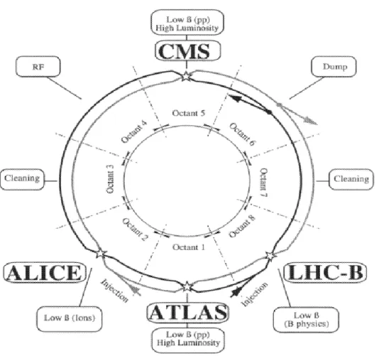
The Large Hadron Collider (LHC) at CERN is the largest and the most powerful particle accelerator in the world. The LHC is 27 km ring which provide 14 TeV proton-proton collisions at design luminosity of 1034 cm-2s-1. Inside the LHC, 2808 bunches of up to 1011 protons (p) are collide 40 million times per second. Heavy ions (A) are also collide inside the LHC ring, in particular lead nuclei, a center of mass energy of 5.5 TeV per nucleon pair, at a design luminosity of 1027 cm-2s-1.
Accelerators at CERN boost particles to high energies, and two high-energy particle beams travel in opposite directions to collide at four locations around the LHC ring, corresponding to the positions of four particle detectors: ATLAS (A Toroidal LHC ApparatuS), CMS (Compact Muon Selenoid), ALICE (A Large Ion Collider Experiment), LCHb (Large Hadron Collider beauty Experiment) (CERN 2013).
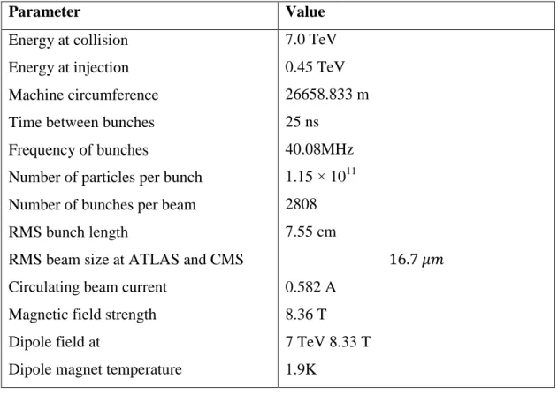
Table 4.1: Some basic parameters of the LHC at design luminosity
Parameter Value
Energy at collision Energy at injection Machine circumference Time between bunches Frequency of bunches
Number of particles per bunch Number of bunches per beam RMS bunch length
RMS beam size at ATLAS and CMS Circulating beam current
Magnetic field strength Dipole field at
Dipole magnet temperature
7.0 TeV 0.45 TeV 26658.833 m 25 ns 40.08MHz 1.15 × 10¹¹ 2808 7.55 cm 0.582 A 8.36 T 7 TeV 8.33 T 1.9K
THE LARGE HADRON COLLIDER(LHC)
24 Number of dipole magnets
Number of quadrupole magnets
1232 392
Figure 4.1. Schematic layout of the LHC
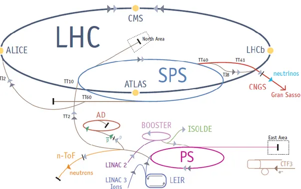
4.1.1 The CERN Accelerator Complex
The CERN accelerator complex is a sequence of particle accelerators as shown in Figure 4.2. Each machine boosts the energy of particle beams to increasingly higher energies, before injecting the beams into the next machine in the sequence. The LHC is the last element in this chain. (LHC Study Group 1995)
25
(CERN 2013) (CERN Communication Group 2009) The proton source is a bottle containing hydrogen gas. The hydrogen bottle is surrounded with an electric field to strip hydrogen atoms of their electrons to yield protons. Linac2 is the first accelerator in the chain, which accelerates the protons to the energy of 50 MeV. The beam is injected into the Proton Synchrotron Booster (PSB) from Linac2. The booster accelerates the protons to 1.4 GeV. The beam is then fed to Proton Synchrotron (PS), which boosts the beam to 25 GeV. The beam is then fed to the Super Proton Synchrotron (SPS), which accelerates the beam to 450 GeV. The beams are finally transferred to the two beam pipes of the LHC where they are circulated for 20 minutes to reach their nominal energy of 7 TeV in opposite direction.
Figure 4.2.CERN accelerator complex
(LHC Study Group1995) The accelerator complex also includes the Antiproton Decelerator (AD) and the Online Isotope Mass Separator (ISOLDE) facility, and feeds the CERN Neutrinos to Gran Sasso (CNGS) project and the Compact Linear Collider test area, as well as the neutron tome-of-flight facility (nTOF).
THE LARGE HADRON COLLIDER(LHC)
26 4.2 The Atlas Detector
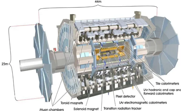
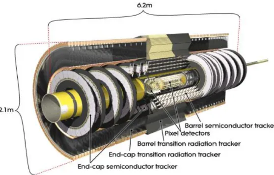
(The ATLAS Collaboration 2008)The ATLAS (A Toroidal LHC ApparatuS) is a general purpose detector which have been built for observation p-p and A-A collisions. The ATLAS is 44m in length, 25m in height, and the weight of the detector is approximately 7000 tones.
The ATLAS detector consists of four main components: Inner Detector (ID), Calorimeter, Muon Spectrometer and Magnet System. The main components of ATLAS detector are shown in Figure 4.3 and the required resolution and the pseudorapdity coverage of these layers are summarized in Table 4.2. The ID is designed to provide excellent momentum resolution and to measure both primary and secondary vertex for charged particles. The Calorimeter is designed to provide electromagnetic and hadronic energy measurements. The Moun Spectrometer identifies and measures the momentum of the mouns. Magnet System bends charged particles for momentum measurements.
General requirements for particle-identification capabilities of the ATLAS detector are:
High detector granularity is needed to handle the particle fluxes and to reduce the influence of overlapping events.
Large acceptance in pseudorapidity with almost full azimuthal angle coverage is required.
Good charged-particle momentum resolution and reconstruction efficiency in the inner detector are essential.
Very good electromagnetic (EM) calorimeter for electron and photon identification and measurements, complemented by full-coverage hadronic calorimeter for accurate jet and missing transverse energy measurements, are important requirements.
Good muon identification and momentum resolution over a wide range of momenta and the ability to determine unambiguously the charge of high transverse-momentum (pT) muons are required.
Highly efficient triggering on low transverse-momentum objects with sufficient background rejection is required.
27
The overall layout of the ATLAS detector is illustrated in Figure 4.3 and its main performance goals are listed in Table 4.1.
Figure 4.3 Cut-away view of the ATLAS detector. (http://atlas.ch/)
Table 4.2 General performance goals of the ATLAS detector.
Detector Component Required resolution coverage
Measurement Trigger
Inner Detector ⁄ ±2.5
EM calorimetry ⁄ √ ⁄ ±3.2 ±2.5
Hadronic calorimetry (jets) barrel and end-cap forward ⁄ √ ⁄ ⁄ √ ⁄ ±3.2 3.1 < < 4.9 ±3.2 3.1< <4.9 Muon spectrometer ⁄ ±2.7 ±2.4
THE LARGE HADRON COLLIDER(LHC)
28
(The ATLAS Collaboration 2008) The center of the ATLAS detector is defined as the nominal interaction point which is the origin of the coordinate system. The z-axis is defined as the parallel to the beam direction, the positive x-axis is defined as the direction from interaction point to the center of LHC ring and the positive y-axis is defined as the perpendicular to the x-z plane and pointing upward. The azimuthal angle 𝜙 is measured as the angle between the particle momentum and the transverse momentum ( ) which depends only x-axis and y-axis, and the polar angle θ is the angle between particle momentum and beam axis. The pseudorapidity is calculated as ⁄ (the rapidity ⁄ ⁄ is used for massive particles such a jets.). The transverse momentum pT, and the
transverse energy ET are defined in the x-y plane. The distance ∆R in the
pseudorapidity-azimuthal angle space is calculated as √ 𝜙 .
4.2.2 Inner Detector
(The ATLAS Collaboration 2008) The ATLAS Inner detector (ID) is designed to provide pattern recognition, excellent momentum resolution and both primary and secondary vertex measurements for charged tracks within the psudorapidity range . It also provides electron identification over . These are achieved with a combination of discrete, high-resolution pixel and silicon microstrip (SCT) trackers in the inner part of the tracking volume and straw tubes of the Transition Radiation Tracker (TRT) with the capability to generate and detect transition radiation in its outer part.
29
Figure 4.4 Cut-away view of the ATLAS inner detector. (http://atlas.ch/)
The layout of the ID is shown in Figure 4.4 and its main parameters and each sub-detector are listed in Table 4.3. The ID is immersed in a 2 T selenoidal magnetic field, which extends over a 5.3 m in length with 2.5 m in diameter. The precision tracking detectors (pixels and SCT) cover the pseudorapidity range . In the barrel region, they are placed on concentric cylinders around the beam axis while in the end-cap region, they are located on disks perpendicular to the beam axis. The highest granularity is achieved around the vertex region using silicon pixel detectors. The pixel layers are segmented in 𝜙 and with typically three pixel layers crossed by each track. All pixel sensors are identical and have a minimum pixel size in 𝜙 of 50 400 . The intrinsic accuracies in the barrel are 10 ( 𝜙) and 115 ( ) and in the disks are 10 ( 𝜙) and 115 ( ). The pixel detector has approximately 80.4 million readout channels. For the SCT, eight strip layers (four space points) are crossed by each track. In the barrel region, this detector uses small-angle (40 mrad) stereo strips to measure both coordinates, with one set of strips in each layer parallel to the beam direction, measuring 𝜙. They consist of two 6.4 cm long daisy-chained sensors with a strip pitch of 80 . In the end-cap region, the detectors have a set of strips running radially and a set of stereo strips at an angle of 40 mrad. The mean pitch of the strips is also approximately
THE LARGE HADRON COLLIDER(LHC)
30
80 . The intrinsic accuracies per module in the barrel are 17 ( 𝜙) and 580 ( ) and in the disks are 17 ( 𝜙) and 580 ( ). The total number of readout channels in the SCT is approximately 6.3 million.
A large number of hits (typically 36 per track) is provided by the 4 mm diameter straw tubes of the TRT, which enables track-following up to . The TRT only provides 𝜙 information, for which it has an intrinsic accuracy of 130 per straw. In the barrel region, the straws are parallel to the beam axis and are 144 cm long, with their wires divided into two halves, approximately at . In the end-cap region, the 37 cm long straws are arranged radially in wheels. The total number of TRT readout channels is approximately 351,000.
Table 4.3 Main parameters of the ATLAS inner-detector system.
Item Radial extension (mm) Length (mm)
Overall ID envelope Beam-pipe
Pixel Overall envelope 3 cylindrical layers Sensitive barrel 2 x 3 disks Sensitive end-cap
SCT Overall envelope
4 cylindrical layers Sensitive barrel 2 x 9 disks Sensitive end-cap
TRT Overall envelope
73 straw planes Sensitive barrel 163 straw planes Sensitive end-cap
(barrel) (end-cap) (barrel) (end-cap)
The combination of precision trackers at small radii with the TRT at a larger radius gives very robust pattern recognition and high precision in both 𝜙 and
31
coordinates. The straw hits at the outer radius contribute significantly to the momentum measurement, since the lower precision per point compared to the silicon is compensated by the large number of measurements and longer measured track length.
The inner detector system provides tracking measurements in a range matched by the precision measurements of the electromagnetic calorimeter. The electron identification capabilities are enhanced by the detection of transition-radiation photons in the xenon-based gas mixture of the straw tubes. The semiconductor trackers also allow impact parameter measurements and vertexing for heavy-flavor and τ-lepton tagging. The secondary vertex measurement performance is enhanced by the innermost layer of pixels, at a radius of about 5 cm.
4.2.3 Calorimeter
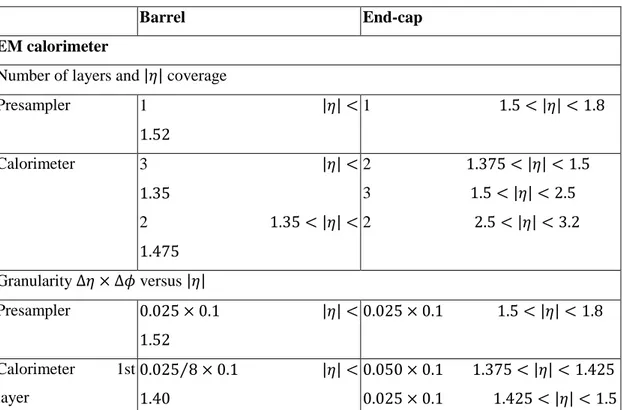
(The ATLAS Collaboration 2008) A cut-away view of the ATLAS calorimeter system is illustrated in Figure 4.5 and the pseudorapidity coverage, granularity and segmentation in depth of the calorimeters are listed in Table 4.4.
The ATLAS calorimeters consist of a number of sampling detectors with full 𝜙-symmetry and coverage around the beam axis. The calorimeters closest to the beam-line are housed in three cryostats, one barrel and two end-caps. The barrel cryostat contains the electromagnetic barrel calorimeter, whereas the two end-cap cryostats each contain an electromagnetic end-cap calorimeter (EMEC), a hadronic end-cap calorimeter (HEC), located behind the EMEC, and a forward calorimeter (FCal) to cover the region closest to the beam. All these calorimeters use liquid argon as the active detector medium; liquid argon has been chosen for its intrinsic linear behavior, its stability of response over time and its intrinsic radiation-hardness.
THE LARGE HADRON COLLIDER(LHC)
32
Figure 4.5 Cut-away view of the ATLAS calorimeter system. (http://atlas.ch/)
Table 4.4 Main parameter of the ATLAS calorimeter system.
Barrel End-cap
EM calorimeter
Number of layers and coverage
Presampler 1 1 Calorimeter 3 2 2 3 2 Granularity 𝜙 versus Presampler Calorimeter 1st layer ⁄
33 ⁄ ⁄ ⁄ Calorimeter 2nd layer Calorimeter 3rd layer
Number of readout channels Presampler Calorimeter 7808 101760 1536 (both sides) 62208 (both sides) LAr hadronic end-cap
coverage Number of layers 4 Granularity 𝜙
Readout channels 5632 (both sides)
LAr forward calorimeter coverage Number of layers 3 Granularity (cm) FCal1: FCal1:~4 t.f. FCal2: FCal2:~4 t.f. FCal3: FCal3:~4 t.f.
Readout channels 3524 (both sides)
Scintillator tile calorimeter
THE LARGE HADRON COLLIDER(LHC) 34 coverage Number of layers 3 3 Granularity 𝜙 Last layer
Readout channels 5760 4092 (both sides)
The precision electromagnetic calorimeters are lead-liquid argon detectors with accordion-shape absorbers and electrodes. This geometry allows the calorimeters to have several active layers in depth, three in the precision-measurement region ( ) and two in the higher- region ( ) and in the overlap region between the barrel and the EMEC. In the precision measurement region, an accurate position measurement is obtained by finely segmenting the first layer in . The -direction of photons is determined by the position of the photon cluster in the first and the second layers. The calorimeter system also has electromagnetic coverage at higher ( ) provided by the FCal. Furthermore in the region ( ) the electromagnetic calorimeters are complemented by presamplers, an instrumented argon layer, which provides a measurement of the energy lost in front of the electromagnetic calorimeters.
For the outer hadronic calorimeter, the sampling medium consists of scintillator tiles and the absorber medium is steel. The tile calorimeter is composed of three parts, one central barrel and two extended barrels. The choice of this technology provides maximum radial depth for the least cost for ATLAS. The tile calorimeter covers the range (central barrel and extended barrels). The hadronic calorimetry is extended to larger pseudorapidities by the HEC, a copper/liquid-argon detector, and the FCal, a copper-tungsten/liquid-argon detector. The hadronic calorimeter thus reaches one of its main design goals, namely coverage over .
35 4.2.4 Muon Spectrometer
(The ATLAS Collaboration 2008) The Muon spectrometer forms the outer part of the ATLAS detector and is designed to detect charged particles exiting the barrel and end-cap calorimeters and to measure their momentum in the pseudorapidity range . It is also designed to trigger on these particles in the region .
The conceptual layout of the muon spectrometer is shown in Figure 4.6 and the main parameters of the muon chambers are listed in Table 4.5. It is based on the magnetic deflection of muon tracks in the large superconducting air-core toroid magnets, instrumented with separate trigger and high-precision tracking chambers. Over the range , magnetic bending is provided by the large barrel toroid. For , muon tracks are bent by two smaller end-cap magnets inserted into both ends of the barrel toroid. Over , usually referred to as the transition region, magnetic deflection is provided by a combination of barrel and end-cap fields. This magnet configuration provides a field which is mostly orthogonal to the muon trajectories, while minimizing the degradation of resolution due to multiple scattering.
THE LARGE HADRON COLLIDER(LHC)
36
Table 4.5 The main parameters of the muon chambers
Drift Tubes MDTs Coverage Number of chambers Number of channels 1170 354000 Cathode Strip Chambers
Coverage Number of chambers Number of channels 32 31000 Resistive Plate Coverage Number of chambers Number of channels 1112 374000 Thin Gap Chambers
Coverage Number of chambers Number of channels 1578 322000
In the barrel region, tracks are measured in chambers arranged in three cylindrical layers around the beam axis; in the transition and end-cap regions, the chambers are installed in planes perpendicular to the beam, also in three layers.
4.2.4.1 The toroidal magnets
(The ATLAS Collaboration 2008) A system of three large air-core toroids generates the magnetic field for the muon spectrometer. The two end-cap toroids are inserted in the barrel toroid at each end and line up with the central solenoid. Each of the three toroids consists of eight coils assembled radially and symmetrically around the beam axis. The end-cap toroid coil system is rotated by 22.5˚ with respect to the barrel toroid coil system in order to provide radial overlap and to optimize the bending power at the interface between the two coil systems.
37
The performance in terms of bending power is characterized by the field integral , where B is the field component normal to the muon direction and the integral is computed along an infinite-momentum muon trajectory, between the innermost and outermost muon-chamber planes. The barrel toroid provides 1.5 to 5.5 Tm of bending power in the pseudorapidity range , and the end-cap toroids approximately 1 to 7.5 Tm in the region . The bending power is lower in the transition regions where the two magnets overlap ( ).
4.2.4.2 Muon chamber types
(The ATLAS Collaboration 2008) Over most of the -range, a precision measurement of the track coordinates in the principal bending direction of the magnetic field is provided by Monitored Drift Tubes (MDT’s). The mechanical isolation in the drift tubes of each sense wire from its neighbors guarantees a robust and reliable operation. At large pseudorapidities, Cathode Strip Chambers (CSC’s, which are multi-wire proportional chambers with cathodes segmented into strips) with higher granularity are used in the innermost plane over , to withstand the demanding rate and background conditions. The stringent requirements on the relative alignment of the muon chamber layers are met by the combination of precision mechanical-assembly techniques and optical alignment systems both within and between muon chambers.
The trigger system covers the pseudorapidity range . Resistive Plate Chambers (RPC’s) are used in the barrel and Thin Gap Chambers (TGC’s) in the end-cap regions. The trigger chambers for the muon spectrometer serve a threefold purpose which is that providing bunch-crossing identification, providing well-defined thresholds, and measuring the muon coordinate in the direction orthogonal to that determined by the precision-tracking chambers.
DATA ANALYSIS AND RESULTS
39 CHAPTER 5
DATA ANALYSIS AND RESULTS 5.1 Overview
In this chapter, we first analyse Atlas 2012 real data by using ROOT . We compare Atlas real data (DA) with MonteCarlos (MC) simulation data prepared according to Atlas real data.
Atlas real data is prepared by Atlas detector in the LHC. It consists of some vectors such as MonteCarlos, Tracks, Conversions and CaloClusters. These are vectors include information about particles detected in Atlas. Tracks has information about charged particle. Conversions has information about electrons and positrons. CaloClusters has information about photons. MonteCarlos has information about all particles but unlike these vectors, it has simulation data prepared according to real data. Some parameters of Atlas data is drawn in the Table 5.1.
Monte Carlo (MC) methods are stochastic techniques--meaning they are based on the use of random numbers and probability statistics to investigate problems. It is found MC methods used in everything from economics to nuclear physics to regulating the flow of traffic. Of course the way they are applied varies widely from field to field, and there are dozens of subsets of MC even within chemistry. But, to call something a "Monte Carlo" experiment, all you need to do is use random numbers to examine some problem.
The use of MC methods to model physical problems allows us to examine more complex systems than we otherwise can. Solving equations which describe the interactions between two atoms is fairly simple; solving the same equations for hundreds or thousands of atoms is impossible. With MC methods, a large system can be sampled in a number of random configurations, and that data can be used to describe the system as a whole.
"Hit and miss" integration is the simplest type of MC method to understand, and it is the type of experiment used in this lab to determine the energy level population distribution. Before discussing the lab, however, we will begin with a
DATA ANALYSIS AND RESULTS
40
simple geometric MC experiment which calculates the value of pi based on a "hit and miss" integration.
The ROOT system provides a set of object-oriented frameworks needed to handle and analyze large amounts of data in a very efficient way. It includes histograming methods, curve fitting, function evaluation, minimization, graphics and visualization
classes to allow the easy setup of an analysis system. The command language, the scripting, or macro language and the programming language are all C++. ROOT is an open system that can be dynamically extended by linking external libraries. This makes ROOT a premier platform on which to build data acquisition, simulation and
data analysis systems.
Table 5.1 atlas data parameters (http://www1.gantep.edu.tr/~bingul/hep/atlas.peng.egAOD.html)
: Vertex fit quality.
f1 : fraction of energy reconstructed in the first sampling with E1 the energy reconstructed in all strips belonging to the cluster and E the total energy reconstructed in the electromagnetic calorimeter cluster.
f1core: fraction of the energy reconstructed in the first longitudinal compartment of the electromagnetic calorimeter with the energy reconstructed in 3 strips in η, centered around the maximum energy strip and E the energy reconstructed in the electromagnetic calorimeter.
e2tsts1: Energy of the cell corresponding to second energy maximum in the first sampling.
emins1: Energy reconstructed in the strip with the minimal value between the first and second maximum.
weta1 : Shower width using ± 1 strip around the one with the maximal energy deposit (a total of 3 strips): √ where i is the number of the strip and imax the strip number of the most energetic one.
wtots1 : Shower width determined in a window corresponding to the cluster size (a maximum of , corresponding typically to 40 strips in η) :
√ where i is the strip number and imax the strip
number of the first local maximum.
41
is the energy in strips around the strip with highest energy. emaxs1: Energy of strip with maximal energy deposit .
e233 :Ucalibrated energy (sum of cells) of the middle sampling in a rectangle of size 3x3 (in cell units eta X phi).
e237 :Uncalibrated energy (sum of cells) of the middle sampling in a rectangle of size 3x7 (in cell units eta X phi).
e277 :Uncalibrated energy (sum of cells) of the middle sampling in a rectangle of size 7x7 (in cell units eta X phi).
weta2 : The lateral width is calculated with a window of 3× 5 cells using the energy weighted sum over all cells, which depends on the particle impact point inside the cell √ where is the energy of the i-th cell and is the pseudorapidity of the i-th cell.
widths2: Same as weta2 but without corrections on particle impact point inside the cell.
f3core : fraction of the energy reconstructed in the third compartment of the electromagnetic calorimeter. The energy in the back sampling is the sum of the energy contained in a 3× 3 window around the maximum energy cell. ethad :Transverse energy in the hadronic calorimeters behind the cluster.
ethad1 :Transverse energy in the first sampling of the hadronic calorimeters behind the cluster.
As we specified (in chapter 3) neutral kaons may decay into two or three pions. But we have already known that two pions system carries a parity of +1 and three pions system carries a parity of -1 but both have . Therefore can decay into two pions and can decay into three pions under CP invariance.
So the neutral kaons provide a perfect experimental system for testing CP invariance. On the other hand by using an enough long beam, we can produce an arbitrarily pure sample of the long-lived species. If at the this point we can observe that decays into , we know that CP has been violated. In the same way we
DATA ANALYSIS AND RESULTS
42
can look at the short-lived kaons. If we can observe that decays into we can say CP is violated.
In this thesis, we look for decayed into We try to find come from and calculate the invariant mass of these three pions. If the invariant mass of these three pions is equal to the invariant mass of then we can say that these three pions come from and so CP is violated. But, unfortunately it is not very easy because in the Atlas Detector neutral pions cannot be observed directly. This is due to fact that neutral pions have very short life time and they decay into other particles. Most common decay mode is two photons decay. Thus, we need to reconstruct pions by using photons. But like pions we also cannot detect photons unless they interact with a matter or a particle.
In the Atlas detector we can observe photons after they interact with the matter and also we can observe them in the calorimeter. When photons interact with
43
matter they decay into electron and positron pairs. Atlas inner detector saves these pairs with some of their information such as momentum (P), phi ( ), energy (E) etc. Therefore as in the creating pions by using photons, we also have to reconstruct photons by using pairs.
Namely, in this thesis we first reconstruct photons from pairs. To do this, we have Conversion vector which has some direct informations on photons to reconstruct pions and Calocluster vector which has some direct informations on photons which detected by calorimeter, and later we reconstruct pions by using photons and finally we reconstruct kaons from pions.
5.2 Photon Reconstruction
Photons are virtual particles to study in a detector. Photons are the decay product of many important particles such as Higgs boson, neutral pion etc. But as it is mentioned earlier the Atlas detector can detect photons directly in the calorimeter by calculating their energy and also it is able to detect the pairs come from photons and save some information of these pairs. We have to reconstruct photons from pairs but before starting we must know what kinds of information are saved by Atlas inner detector in the conversions vector.
Atlas inner detector saves information in a vector called conversions. Conversions vector has some information (about pairs come from photons) such as phi ( ), eta (η), qoverp (q/p) etc.
By using this information we can reconstruct photons. But we have to do some cuts during the process of recreating photons, namely we have to choose the correct pairs to reconstruct photons. To able to do this, we should know what these cuts are. For example the conversion pairs have different phi2 which is the value that the detector gives to the each particles detected. Detector gives different value numbers to different particles. And if the phi2 value of a pair is equal to -99, this means that this pair did not come from photon, to reconstruct photons you have to eliminate this pair. There are some more cuts such as P(momentum), eta(η), qoverp (q/p) etc.
DATA ANALYSIS AND RESULTS
44
Figure 5.1 value distribution of photons reconstructed from electron and positron pairs for conversions vector
One of the important parameter is the vertex fit quality, . The distribution of is given in Figure 5.1. In Atlas detector is calculated according to conversion candidates. Atlas accepts all charged particles which decayed in the inner detector as that they are coming from photons. Then, Atlas combines their tracks and later fits their vertexs. After these steps it calculated the probability of these particles. If our particles are certainly conversion, then Atlas saves value close to 1. Namely, value is probability of good photon. It is close to 1 for photon. As we see in the graph it goes to more than 50 but the distribution spread between 0 and 5 represents good photons. The rest of distribution represents some particles different from photons and also not good photons for analysis. Thus, in the analysis we will choose from 0 to 10. Because, we want to obtain good photons to reconstruct pions and this interspace will give us good photons.
45
Figure 5.2 Eta (η) value distribution of photon reconstructed form electron and positron pairs for conversions vector
The pseudorapidity of particles from the primary vertex is defined as
where is the polar angle of the particle direction measured from the positive z-axis. Transverse momentum, , is defined as the momentum perpendicular to the LHC beam axis.(http://www.hep.lu.se/atlas/thesis/egede/thesis-node39.html) The distribution of this parameter is exhibited in Figure 5.2. As seen the entries spread from -2.5 to 2.5. It means that detector can detect the particles which have between -2.5 and 2.5. Thus, according to Figure 5.2 we can choose -1.5 to 1.5 because most of particles have value between this spacing.
DATA ANALYSIS AND RESULTS
46
Figure 5.3 q/p value distribution of photon reconstructed from electron and positron pairs for conversions vector
As we see the distribution of electron-positron pairs with respect to q/p around zero. By using q/p we can define the particle if it is positive charged or negative charged. Figure 5.3 shows the distribution of pairs came from photons and by using q/p we can identify if it is electron or positron. In the detector, after photons decay into electron-positron pairs, these pairs go on their way under the electric field. Thus, these pairs are affected from this field and so positive charged particles move to negative side and negative charged particles move to positive side. And detector calculates the momentum of these particles by using their energy and later calculates the ratio of and saves this information in a vector called conversions in the name of q/p.
Namely, the negative value of q/p means that this is electron and the positive is positron. The graph has nearly the same rate of negative and positive value. Because these pairs came from photons and for each decays of photon we get an electron and a positron.
47
Figure 5.4 Momentum distribution of photon reconstructed from electron-positron pairs from conversions vector
The momentum (in ) distribution of photons which are reconstructed from pairs from conversions vector is drawn in Figure 5.4. ın this process we make two different loops. In the first loop we choose an electron and in the second loop we choose a positron corresponding to the electron chosen before in the first loop. And later we combine this pairs to reconstruct photon. After that we calculate energy and momentum of these photons by using the information of these pairs. It is drawn to compare the momentum of photons with the energy of photons. By comparing them we know if our reconstruction is correct.