© TÜBİTAK
doi:10.3906/elk-1809-129 h t t p : / / j o u r n a l s . t u b i t a k . g o v . t r / e l e k t r i k /
Research Article
Performance tuning for machine learning-based software development effort
prediction models
Egemen ERTUĞRUL1,, Zakir BAYTAR2,, Çağatay ÇATAL3∗,, Can MURATLI2,
1Department of Computer Science and Engineering, Shanghai Jiao Tong University,Shanghai, P.R. China 2Department of Computer Engineering, Faculty of Engineering, İstanbul Kültür University, İstanbul, Turkey
3Information Technology Group, Social Sciences, Wageningen University, Wageningen, the Netherlands
Received: 18.09.2018 • Accepted/Published Online: 30.12.2018 • Final Version: 22.03.2019
Abstract: Software development effort estimation is a critical activity of the project management process. In this
study, machine learning algorithms were investigated in conjunction with feature transformation, feature selection, and parameter tuning techniques to estimate the development effort accurately and a new model was proposed as part of an expert system. We preferred the most general-purpose algorithms, applied parameter optimization technique (Grid-Search), feature transformation techniques (binning and one-hot-encoding), and feature selection algorithm (principal component analysis). All the models were trained on the ISBSG datasets and implemented by using the scikit-learn package in the Python language. The proposed model uses a multilayer perceptron as its underlying algorithm, applies binning of the features to transform continuous features and one-hot-encoding technique to transform categorical data into numerical values as feature transformation techniques, does feature selection based on the principal component analysis method, and performs parameter tuning based on the GridSearch algorithm. We demonstrate that our effort prediction model mostly outperforms the other existing models in terms of prediction accuracy based on the mean absolute residual parameter.
Key words: Software effort estimation, machine learning, feature binning, grid search, artificial neural networks, mean
absolute residual
1. Introduction
The effort required for the development of a software project can change with many factors in the development. While this effort can be predicted by using several methods, prediction results can lead to either underestimation or overestimation. Predicting the effort in an accurate way can help software companies foresee the costs in an effective manner. The total project effort and the associated cost needed for the development should be estimated accurately before the software project is carried out. This is one of the most important main tasks of the software project manager. These estimations are used to determine the necessary resources (i.e. the budget for human resources, number of personnel), project plans, schedules, bidding processes, milestones, and deadlines. If the effort required for the project development is predicted incorrectly, then the cost of the software development process might be underestimated or overestimated, both having negative effects by causing the company to lose profit or visibility. Therefore, software development effort estimation (SDEE) is a crucial step in the early stages of the software development life cycle to avoid unexpected situations that might arise.
Effort estimation in software development is a research topic that has been studied and improved since
∗Correspondence: [email protected]
the mid-1960s [2, 3]. Since then, there have been numerous methods, techniques, and tools that emerged to address the problem of effort estimation. Estimation techniques that are used nowadays by the software cost
predictors can be divided into three main groups [1,5]:
• expert judgment,
• algorithmic/parametric models, and • machine learning models.
Expert judgment is realized with the help of an expert who uses his/her knowledge and expertise on
estimating the project effort during the project management activities [1, 8]. Algorithmic models (a.k.a.
parametric models) such as the popular COCOMO model, SEER-SEM, and SLIM mostly apply function point (FP) measure and source lines of code (SLOC) metric values to calculate the development effort. Finally,
machine learning models, which can be used either standalone or in conjunction with algorithmic models [1],
can be built by using machine learning algorithms such as naive Bayes and decision trees.
In this study, we aimed to develop a novel machine learning-based software effort estimation model by using not only feature transformation and feature selection techniques but also parameter tuning techniques on datasets created based on real software development projects. We also intended to investigate the effectiveness of commonly used machine learning algorithms on the estimation of software development effort. To achieve this, we implemented nine machine learning regression models to evaluate the prediction accuracy on the software development effort, compared the test results with the best results reported in the literature, and worked on the optimum parameter values of each model. In order to compare our results with the research results obtained
recently by Nassif et al. [1], we used the same set of datasets and performance evaluation criterion. Datasets
used to train and test our models were retrieved from the International Software Benchmarking Standards
Group (ISBSG) [10] and contain the following features that might affect the effort estimation [9]:
• adjusted function points (AFP): continuous feature, • development platform: categorical feature,
• language type: categorical feature, • resource level: categorical feature, • effort: output value.
The first four features are used as the input features and the last one (effort) is considered the output value, which must be estimated accurately. Our main performance evaluation criterion for the machine learning-based models is mean absolute residual (MAR), which is explained by the datasets in Section 3 in detail. We identified the following research questions (RQs) for this research:
• RQ1: Which machine learning algorithm provides the best performance in terms of mean absolute residual parameter?
• RQ2: Which machine learning algorithm tends to overestimate and which tends to underestimate? • RQ3: Can we build better machine learning-based models in terms of prediction accuracy by applying
The remaining sections of this paper are as follows: Section2 gives a brief overview of the related work
and background. Section 3 describes the evaluation performance criterion and datasets, and explains how we
trained and tested machine learning models and optimized the parameters. Section4shows the test results and
discussions. Section5 lists the threats to the validity, which are critical for any experimental research. Finally,
Section 6explains the conclusions and future work.
2. Related work
The majority of the previous studies developed effort estimation models based on machine learning algorithms
such as artificial neural networks, genetic algorithms, support vector machines, and decision trees [4]. In this
section, we investigate the previous studies that applied general-purpose regression algorithms to build software effort estimation models.
A systematic review paper was published by Jorgensen and Shepperd [6]. They identified 304 papers in
2007 that are all relevant to software cost estimation and classified these papers to provide a perspective and support as recommendations for future cost-estimation researchers. This systematic review paper was different than the previous review papers on software effort estimation because it included a systematic selection process and more papers compared to other review articles. They also classified papers based on several dimensions such as study context, dataset, and estimation topics. In a more recent systematic review paper, Wen et al.
[4] identified 84 primary studies about machine learning-based software effort estimation between 1991 and
2010, and they reported that they identified eight types of machine learning techniques that were used in effort estimation studies. It was seen that applications of machine learning (ML) techniques in the software development effort estimation (SDEE) domain was launched by the 1990s. It was concluded that the estimation accuracy of the ML models that were investigated is better than that of non-ML models.
Sehra et al. [7] semantically mapped 1178 papers about SDEE published between 1996 and 2016 by
employing natural language processing in order to help researchers in finding the potential research areas on SDEE. They reported that the number of papers published about ML-based SDEE significantly increased over the last two decades. This indicates that machine learning-based effort estimation studies still have much potential for novel models when considering the better predictive accuracy.
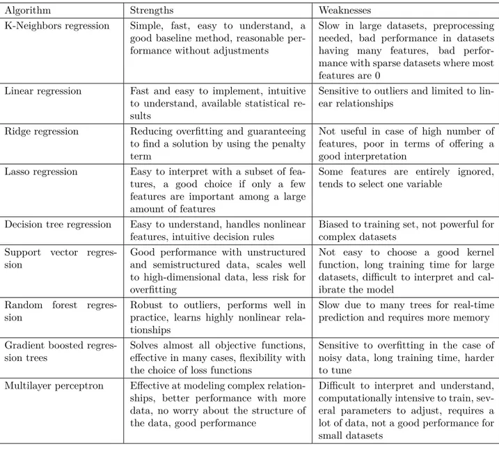
In Table 1, we explain the strengths and weaknesses of the following machine learning algorithms in
the context of software development effort estimation models to provide a comprehensive comparison and then we provide the relevant literature for each of these algorithms: K-nearest neighbors, linear regression, ridge regression, lasso regression, decision tree regression, support vector regression, random forest regression, gradient boosted regression trees, and multilayer perceptron (MLP).
Kocaguneli et al. [15] employed kNN with a certain number of “k”s and the Best(K) method in order to
estimate software development effort accurately on nine datasets including one ISBSG dataset. They concluded that estimation by analogy approach provides better results when selecting neighbors from regions with small variance. A limitation to mention about this technique is that it cannot predict a value on a dimension that
is outside the range of values in the training data such as the software development effort [14]. Other similar
limitations may apply to this technique. Menzies et al. [16] and Sarro et al. [18] used the automatically
transformed linear baseline model (ATLM), a multiple linear regression model that was proposed by Whigham
et al. [17]. ATLM is considered to be performing well over different project types and it is easy to deploy with no
parameter tuning. Shahpar et al. [19] used a binary genetic algorithm for feature selection before investigating
Table 1. Comprehensive comparison of deployed machine learning algorithms for software effort estimation.
Algorithm Strengths Weaknesses
K-Neighbors regression Simple, fast, easy to understand, a
good baseline method, reasonable per-formance without adjustments
Slow in large datasets, preprocessing needed, bad performance in datasets having many features, bad perfor-mance with sparse datasets where most features are 0
Linear regression Fast and easy to implement, intuitive
to understand, available statistical re-sults
Sensitive to outliers and limited to lin-ear relationships
Ridge regression Reducing overfitting and guaranteeing
to find a solution by using the penalty term
Not useful in case of high number of features, poor in terms of offering a good interpretation
Lasso regression Easy to interpret with a subset of
fea-tures, a good choice if only a few features are important among a large amount of features
Some features are entirely ignored, tends to select one variable
Decision tree regression Easy to understand, handles nonlinear
features, intuitive decision rules
Biased to training set, not powerful for complex datasets
Support vector regres-sion
Good performance with unstructured and semistructured data, scales well to high-dimensional data, less risk for overfitting
Not easy to choose a good kernel function, long training time for large datasets, difficult to interpret and cal-ibrate the model
Random forest regres-sion
Robust to outliers, performs well in practice, learns highly nonlinear rela-tionships
Slow due to many trees for real-time prediction and requires more memory Gradient boosted
regres-sion trees
Solves almost all objective functions, effective in many cases, flexibility with the choice of loss functions
Sensitive to overfitting in the case of noisy data, long training time, harder to tune
Multilayer perceptron Effective at modeling complex
relation-ships, better performance with more data, no worry about the structure of the data, good performance
Difficult to interpret and understand, computationally intensive to train, sev-eral parameters to adjust, requires a lot of data, not a good performance for small datasets
applied log-linear regression (LLR) [30,35]. Dejaeger et al. [20] investigated the ridge regression model with 12
other models and tested these models over 9 datasets including ISBSG. Li et al. [21] proposed an adaptive ridge
regression system, which is an integration of data transformation, multicollinearity diagnosis, ridge regression technique, and multiobjective optimization. In the study, it was concluded that the adaptive ridge regression system that they proposed can significantly improve the performance of regressions on multicollinear datasets
and produce more explainable results than machine learning methods. Papatheocharous et al. [22] deployed
ridge regression with the genetic algorithm and compared it with the other ML techniques. Another researcher
also focused on ridge regression [23]. Nguyen et al. [23] proposed a constrained regression technique and
compared the prediction accuracy of this technique with the lasso, ridge regression, and other techniques by
the evolution of a decision-tree algorithm instead of the decision tree itself. Shahpar et al. [19] tested decision
trees over three datasets and Sarro et al. [18] deployed decision trees to test on five datasets. Oliveira [26]
applied support vector regression with the linear kernel as well as RBF kernel. It was concluded that SVR outperformed radial basis functions neural networks (RBFNs) and linear regression when analyzed on a dataset
from NASA. In another study, Oliveira et al. [27] observed that the proposed GA-based method increased the
performance of SVR (RBF and linear kernels). It was also stated that in methods such as MLP, RBF, and SVR, the level of accuracy in software effort estimation heavily relies on the values of the parameters. Lin et
al. [28] proposed a model combining GA with SVR and tested the model on COCOMO, Desharnais, Kemerer,
and Albrecht datasets. Dejaeger et al. [20] concluded that nonlinear techniques such as SVM, RBFN, and
MLP did not perform well on large datasets such as ISBSG datasets. However, LS-SVM performed relatively
better. Corazza et al. [29] applied SVR with 18 configurations with the leave-one-out (LOO) cross-validation
approach. Random forest (RF) algorithms are usually applied in fault prediction models. In a recent study
performed by Satapathy et al. [30], the RF technique was employed to test and enhance the prediction accuracy
of software effort estimation by utilizing the use case point (UCP) approach. Test results were compared with MLP, RBFN, SGB, and LLR techniques. As a result, it was stated that the RF technique had lower MMRE
and therefore higher accuracy was achieved in the estimation of software development effort. Nassif et al. [31]
proposed a TreeBoost (stochastic gradient boosting) model to predict software effort based on the UCP method. The TreeBoost model was later compared with a multiple regression model by using four performance criteria:
MMRE, PRED, MdMRE, and MSE. Elish [32] evaluated the potential of multiple additive regression trees
(MARTs) proposed by Friedman [33] as a software effort estimation model. MLP is one of the most applied
techniques in SDEE and it is considered the state-of-the-art [4] algorithm for this problem. MLP is generally
compared with the other systems. In a recent work, Nassif et al. [1] tested and compared the MLP technique
on ISBSG datasets by using the MAR evaluation parameter. There are several researchers who applied MLP in their studies [20,27,30,34–36].
3. Methodology
The datasets we used to train our models were retrieved from the International Software Benchmarking
Standards Group (ISBSG) [10]. These datasets are a part of the ISBSG Release 11 datasets, which consist
of data from 5052 IT projects from all around the world. These datasets helped us to perform an unbiased
comparison between our models and the models suggested in the literature. Nassif et al. [1] provided a
replicable algorithm that filters ISBSG Release 11 datasets into five datasets based on the productivity factor of the projects. If the projects were not categorized using the productivity, the models would not provide high performance because of the different features of the projects. To compare the results of our models with the
results in the literature, we investigated the results of Nassif et al. [1]. Our aim was to find a novel effort
estimation model that can estimate the effort better than the best model reported in the study of Nassif et al. [1].
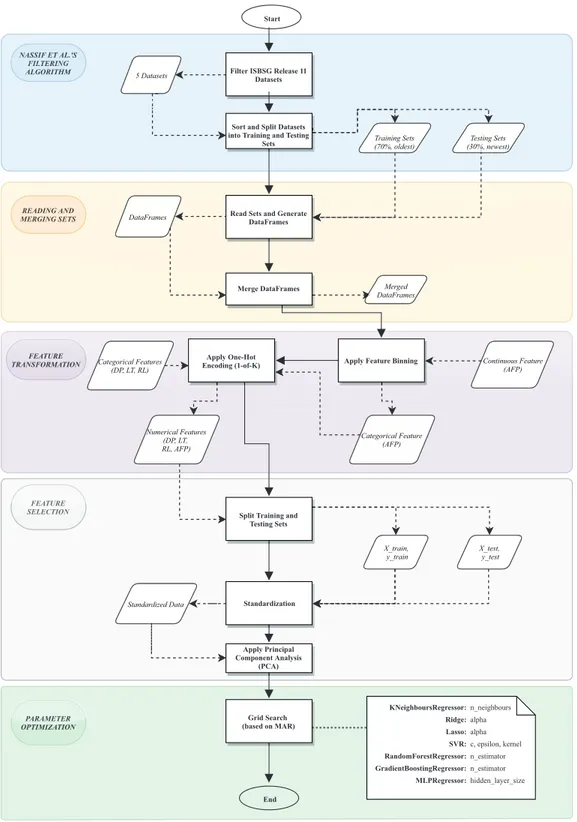
Figure1shows the general methodology of this study, which has five major steps: filtering the datasets,
reading and merging datasets, feature transformation, feature selection, and parameter optimization.
In all the datasets, there were the following sets of features: adjusted function points (AFP), development type (DT), development platform (DP), language type (LT), resource level (RL), and effort (E). DT was chosen as “new development” by default instead of “enhancement” type. This means that all the experiments
Filter ISBSG Release 11 Datasets
Sort and Split Datasets into Training and Testing
Sets Start
Read Sets and Generate DataFrames
Merge DataFrames
Apply One-Hot Encoding (1-of-K)
Split Training and Testing Sets
Grid Search (based on MAR)
Apply Feature Binning
DataFrames 5 Datasets Training Sets T T (70%, oldest) Testing Sets T T (30%, newest) (30%, newest) (30%, newest) Merged Mer Mer DataFrames Continuous Featureurur (AFP) Categ Categorical Featur Categ Categ turtures
(DP, L (DP (DP T, RL)TT Categorical Feature Categorical Featur Categorical Featur (AFP) Numerical Featur Numerical Featur Numerical Featur Numerical Features Numerical Featur Numerical Featur (DP, L (DP (DP T, TT RL, AFP) X_train, y_train X_test, y_test Standardization Apply Principal Component Analysis (PCA) Standardized Data Standar Standar End NASSIF ET AL.'S FIL FILTERINGTERING ALGORITHM READING AND MERGING SETS FEATURE SELECTION SELECTIO FEA FEA FEATURETURETURE TRANS TRANSFORMAFORMATIONTION
KNeighboursRegressor: n_neighbours Ridge: alpha Lasso: alpha SVR: c, epsilon, kernel RandomForestRegressor: n_estimator GradientBoostingRegressor: n_estimator MLPRegressor: hidden_layer_size PARAMETER P P OPTIMIZA OPTIMIZATION
Figure 1. The proposed framework of our prediction approach.
were performed on new software development projects instead of enhancement projects. Since all the projects contained the same value for DT, it was discarded and not used for the training of the models. Each dataset was sorted based on the project implementation year and split into the training and test sets. The training
dataset is the oldest 70% and the testing set is the most recent 30% of the corresponding sorted dataset. This
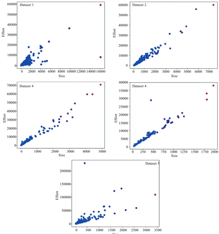
approach was also followed by Nassif et al. [1]. Figure2 shows the scatter plots of five filtered datasets with
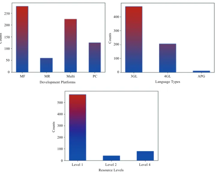
the continuous features of the dataset, namely AFP and effort. Figure 3 shows the count of each categorical
feature (DT, LT, RL) in the whole filtered dataset.
60000 50000 40000 30000 20000 10000 0 0 2000 4000 6000 8000 10000 12000 14000 16000 0 1000 2000 3000 4000 5000 6000 7000 0 10000 20000 30000 40000 50000 60000 0 1000 2000 3000 4000 5000 0 10000 20000 30000 40000 50000 60000 70000 0 250 500 750 1000 1250 1500 1750 2000 40000 35000 30000 25000 20000 15000 10000 5000 0 E ff o rt E ff o rt E ff o rt E ff o rt E ff o rt 0 500 1000 1500 2000 2500 3000 3500 200000 150000 100000 50000 0 Size Size Size Size Size Dataset 1 Dataset 2 Dataset 4 Dataset 5 Dataset 4
C o u n ts 250 200 150 100 50 0 C o u n ts 400 300 200 100 0 C o u n ts 400 500 300 200 100 0 Development Platforms MF MR Multi PC 3GL 4GL APG Language Types
Level 1 Level 2 Level 4
Resource Levels
Figure 3. Plots showing the counts of each categorical feature.
Generally speaking, the majority of previous machine learning studies in SDEE selected the mean magnitude of relative error (MMRE) as the main evaluation performance parameter. However, Shepperd and
MacDonell [11] stated that this criterion is biased and Foss et al. [37] concluded that MMRE does not always
select the best model and it is not recommended for use. Therefore, we chose to work with mean absolute
residual (MAR) as performed by Nassif et al. [1]. This parameter lets our research be comparable with the
other studies in this field and helps to perform the unbiased evaluation. The equation of the MAR parameter is given in Eq. (1) as follows:
MAR =|Ea− Ep|
n . (1)
This equation helps us to answer the first research question. In order to answer the second research question, we should focus on the mean of the residuals (MR). While MR with a negative value indicates that
MR parameter is given in Eq. (2) as follows:
MR = Ea− Ep
n . (2)
In Eqs. (1) and (2), Ea is the actual effort, Ep is the predicted effort, and n is the number of observations.
We deployed the scikit-learn [38] library in Python 3.6.2 to test and evaluate the techniques we explained
in Section 2 when estimating software development effort on the dataset we filtered and split. First of all, we read the datasets and generated “DataFrames”. Then these DataFrames were merged in order to solve a couple of problems, given as follows:
• Training and testing sets do not have equal shapes (missing in features) on some occasions. Therefore, when a model is trained, the testing set may become inapplicable.
• Categorical features are needed to be transformed into numerical values and should not be left as plain strings.
After this merging operation was completed, we applied the “get_dummies” method that exists in the library to implement the “One Hot Encoding” approach (a.k.a. 1-of-K representation) to transform each categorical feature (DP, LT, RL) into a numerical value. Since AFP is the only continuous feature, we converted the AFP feature values into categorical features using the “Feature Binning” method, then transformed them into numerical values just like we did for the initial categorical features. The reason behind this binning method is that we wish to have a set of AFP features rather than only one AFP value. Therefore, we can state that One Hot Encoding and Binning approaches were used properly during the experiments as part of the feature
engineering. Previous research performed by Nassif et al. [1] did not apply these approaches.
We split the dataset into the same number of instances in the initial datasets after these preparation steps were accomplished. Each training dataset was split as “X_train (data)” and “y_train (target)” while “target” contained the Effort feature and “data” contained the rest of the features except Effort. The same process was repeated for the testing dataset on X_test and y_test, respectively. The principal component analysis (PCA) method was used on both “data” and “target” to perform feature selection. First, “data” was standardized using the “StandardScaler()” method. Then we used the PCA method on the standardized data (fitting). As the result of PCA, the “explained_variance” values that are larger than 1 are equal to the “n_componentv of the PCA that we actually aim to apply. At the end of this feature selection process, we enabled data to be used in all of our regression methods.
We found the best parameters by evaluating different values and investigating the MAR results in the following methods:
• KneighborsRegressor: n_neighbors • Ridge: alpha
• Lasso: alpha
• SVR: c, epsilon, and kernel
• RandomForestRegressor: n_estimator • GradientBoostingRegressor: n_estimator • MLPRegressor: hidden_layer_size
LinearRegressor did not have any changed parameters. Default parameters provided the best results and this was noticed when a cross-validation method was applied. DecisionTreeRegressor’s “criterion” parameter was changed to “mae (mean absolute error)” and as the result of cross-validation, it was concluded that the best parameter for “max_features” is “auto” and for “splitter” is “best”. SVR could not be trained on some of the datasets due to the convergence error, thus receiving negative accuracy. GradientBoostingRegressor had its parameter “criterion” changed to “mae”. The following parameters of MLP were changed: “solver” = “lbfgs”
(“sgd” did not produce good results), “max_iter”=10000, “tol”=1e-5 (according to [1]). Finally, all of the
methods we explained were tested on each of the datasets. 4. Experimental results
After we tested all the machine learning models, we calculated their corresponding MAR and MR results. It is worth mentioning that MAR is inversely proportional to the prediction accuracy. Therefore, results with the lowest MAR values are highlighted as the best per dataset. “-” means that the model was not trained properly
and the R2 score was negative. Tables 2 and 3 show the results retrieved from the models tested without
cross-validation applied (Case Study-I).
Table 2. MAR results (Case Study-I).
MAR
Datasets KNN Linear Ridge
1 1647.616279 1683.772604 1624.595153
2 2721.091026 2764.300366 2764.300366
3 - -
-4 725.2944444 946.8369295 639.8974049
5 6768.057143 9324.841774 6414.672678
Datasets Lasso Decision tree SVR
1 1627.509242 - 1443.23369
2 2764.300366 - 2665.013301
3 - -
-4 636.7576608 1728.566667 615.6874255
5 6411.409179 - 4712.439942
Datasets Random forest Gradient boosting MLP
1 1755.745349 1953.560157 1096.184581
2 - - 1048.095695
3 - - 1193.547521
4 1338.866667 1310.793552 876.2732386
5 9793.485714 - 5392.02554
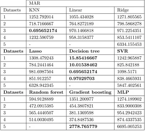
Tables4and5present the results of the models tested with 10-fold cross-validation applied (Case
Study-II). Therefore, we can state that two case studies were performed on the datasets.
In addition to these tables, we provide Tables 6, 7, 8, and 9 to show the difference between our study
and the study of Nassif et al. [1] in terms of MAR and MR values. In these tables, the red circle indicates that
Table 3. MR results (Case Study-I).
MR
Datasets KNN Linear Ridge
1 –1113.267442 –1005.70746 –1005.70746
2 –2721.091026 –2764.300366 –2764.300366
3 - -
-4 295.7722222 324.457277 324.457277
5 –2504.42449 –2339.404082 –2339.404082
Datasets Lasso Decision tree SVR
1 –1005.70746 - –1177.967143
2 –2764.300366 - –2665.013301
3 - -
-4 324.457277 –469.1666667 331.8205759
5 –2339.404082 - 1545.349206
Datasets Random forest Gradient boosting MLP
1 –1205.598837 –1091.967721 112.4739216
2 - - 220.2049275
3 - - 316.1033587
4 –338.8 –325.345565 449.9484135
5 –5800.657143 - 471.6293108
Table 4. MAR results (Case Study-II with 10-fold).
MAR
Datasets KNN Linear Ridge
1 1252.792014 1055.434028 1271.805565
2 718.7166667 764.8272189 798.5868278
3 0.695652174 970.1466818 971.2254351
4 1232.590759 958.3158377 853.5411107
5 - - 6334.155453
Datasets Lasso Decision tree SVR
1 1308.479243 15.85416667 1242.965887
2 784.2441464 10.01538462 825.842188
3 981.6987504 0.695652174 1098.5171
4 851.912257 0.97029703 838.4665931
5 6328.942345 - 5847.402561
Datasets Random forest Gradient boosting MLP
1 594.9128889 1351.200977 1274.189902
2 472.0915385 454.3807821 833.9000308
3 565.4440507 381.1369598 954.2942423
4 514.0030495 374.8487536 874.4337535
Table 5. MR Results (Case Study-II with 10-fold).
MR
Datasets KNN Linear Ridge
1 233.915625 –9.538194444 272.0767273
2 81.39615385 3.74292E-13 –2.430143287
3 0 8.17227E-13 2.20783E-13
4 295.6974697 –7.65416E-14 125.1798687
5 - - 1183.19781
Datasets Lasso Decision tree SVR
1 2.94E-13 0 –181.7864067
2 1.53914E-13 0 –53.99266381
3 1.96398E-12 0 –221.9885122
4 137.2110814 0 249.2351298
5 1216.283188 - 3445.333049
Datasets Random forest Gradient boosting MLP
1 47.20512847 141.2215349 238.6961049
2 –5.398076923 70.27350874 –89.17206537
3 86.41236232 61.7726392 –9.051899616
4 5.09270297 216.3165871 37.34299752
5 - 1752.228688 244.1641233
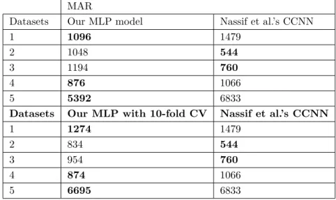
Table 6. Comparison of our MLP model with the CCNN model of Nassif et al. in terms of MAR values.
MAR
Datasets Our MLP model Nassif et al.’s CCNN
1 1096 1479
2 1048 544
3 1194 760
4 876 1066
5 5392 6833
Datasets Our MLP with 10-fold CV Nassif et al.’s CCNN
1 1274 1479
2 834 544
3 954 760
4 874 1066
5 6695 6833
To perform Case Study-II, we combined two datasets (training and testing datasets) to build a whole dataset and applied a 10-fold cross-validation (CV) method. For Case Study-I, we trained our models on the training dataset and evaluated their performances on the testing dataset. Case Study-I is more realistic compared to the second case study because the first case study uses a separate testing dataset instead of
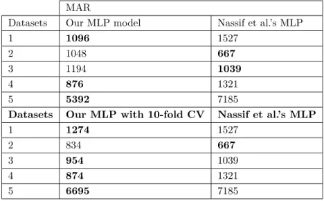
Table 7. Comparison of our MLP model with the MLP model of Nassif et al. in terms of MAR values.
MAR
Datasets Our MLP model Nassif et al.’s MLP
1 1096 1527
2 1048 667
3 1194 1039
4 876 1321
5 5392 7185
Datasets Our MLP with 10-fold CV Nassif et al.’s MLP
1 1274 1527
2 834 667
3 954 1039
4 874 1321
5 6695 7185
Table 8. Comparison of our MLP model with the CCNN model of Nassif et al. in terms of MR values.
MR
Datasets Our MLP model Nassif et al.’s CCNN
1 112 –290
2 220 368
3 316 69
4 450 –771
5 472 –1831
Datasets Our MLP with 10-fold CV Nassif et al.’s CCNN
1 238 –290
2 –89 368
3 –75 69
4 59 –771
5 985 –1831
evaluating data instances on the dataset that was also used for training. Results of the first case study and
second case study were compared with a recent study performed by Nassif et al. [1] and it was shown that our
model provides better performance in terms of MAR values.
As seen in Table 1, our model shown in the MLP column provides the following values in our experiments for the datasets: 1096, 1048, 1193, 876, and 5392, respectively. The suggested algorithm in the paper of Nassif
et al. [1] is CCNN, which provides the following results on the corresponding datasets: 1479, 544, 760, 1066,
and 6833. Based on this comparison, we can state that our new model outperforms the CCNN model in 60%
of the datasets when the MAR parameter is applied. In the study of Nassif et al. [1], the performance of the
MLP model was given as follows: 1527, 667, 1039, 1321, and 7185. Again, our new model performs better than the traditional MLP model in 60% of the datasets. We empirically observed that our model mostly performs better in terms of MAR values on datasets 1, 4, and 5.
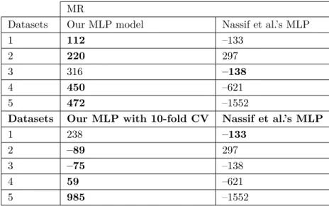
Table 9. Comparison of our MLP model with the MLP model of Nassif et al. in terms of MR values.
MR
Datasets Our MLP model Nassif et al.’s MLP
1 112 –133
2 220 297
3 316 –138
4 450 –621
5 472 –1552
Datasets Our MLP with 10-fold CV Nassif et al.’s MLP
1 238 –133
2 –89 297
3 –75 –138
4 59 –621
5 985 –1552
As shown in Table 3, for Case Study-II (10-fold cross-validation), our model shown in the MLP column provides the following results for all the datasets, respectively: 1274, 833, 954, 874, and 6695. When we compare
these values with the values reported in the study of Nassif et al. [1], we observe that our MLP based model
outperforms the MLP model in that study in 80% of the datasets and our model outperforms the CCNN model in that study in 60% of the datasets. According to these figures and results, the research questions that we proposed at the beginning of this research can be answered as follows:
• RQ1: Which of the machine learning models provides the lowest MAR value?
Our MLP-based model mostly has the lowest MAR values when cross-validation is not applied. Decision tree has the lowest MAR when 10-fold cross-validation is applied. However, the decision tree algorithm seems to provide unrealistic results on the same datasets. Therefore, we suggest the MLP algorithm and the other feature engineering methods we used, namely PCA for feature selection, feature binning to transform continuous data, one-of-K representation to transform categorical data into numerical values, and the GridSearch algorithm for parameter tuning.
• RQ2: Which machine learning model tends to overestimate and which tends to underestimate?
MR results vary on each dataset and on the cross-validation case. Mostly, MLP is underestimating and linear regression is overestimating.
• RQ3: Can we build better machine learning-based models in terms of prediction accuracy by applying feature transformation, feature selection, and parameter tuning techniques?
We demonstrated that better machine learning-based effort estimation models can be built with the help of feature engineering and parameter optimization techniques.
5. Threats to validity
In this section, we evaluated the threats that might affect the validity of the results of this research. These threats can be listed as follows:
1. During our tests, datasets from ISBSG were used and trained. Even though these datasets reflect the state of the art in the software industry, software development scenarios in the world are limitless. Therefore, it is impossible to cover all the cases that might come up. The results that we reached with ISBSG datasets might be different when other datasets are used.
2. MMRE (Mean magnitude of relative error) was not used as a performance evaluation criterion. Instead, MAR (mean absolute residual) was applied. If we had evaluated MMRE results and did not consider
MAR results, then this work would suggest another model. However, as we discussed in Section 3, the
MMRE criterion is a biased parameter and it does not always select the best model. Therefore, it is not suggested for the comparison of effort estimation models.
3. We applied a subset of all the machine learning algorithms reported in the literature and this subset was selected due to their popularity for the underlying problem. We did not cover all the machine learning algorithms during our experiments. Therefore, it is possible that other researchers might end up with better models and techniques.
6. Conclusion and future work
Estimating software effort accurately is very challenging and companies still struggle with this problem. Some software companies still use the approaches proposed in the 1970s during the bidding process, but those techniques, which do not reflect the current state of the art in the software industry, normally fail for reliable estimation. Although it was previously shown that machine learning algorithms have high potential for accurate estimation, there is still a big opportunity for software engineering researchers to develop more accurate effort estimation models as both overestimating and underestimating have detrimental effects for the company.
In this study, we investigated several machine learning algorithms in conjunction with feature selection, feature transformation, and parameter optimization techniques and proposed a new model that provides better prediction performance than the best model reported in the literature. Artificial neural networks, specifically multilayer perceptron topology, helped us to build a high-performance effort estimation model, but additional feature engineering techniques have been integrated to achieve the best performance. Whether we use binning or not, the multilayer perceptron algorithm provides the lowest MAR values, which means that the best algorithm is artificial neural network-based. When we applied PCA for Case Study-I on the feature set, we reached lower MAR results. Since Case Study-I is more realistic when considering the real scenario, we can state that feature selection algorithms also help to build effort estimation models. In addition to the feature selection algorithm, we observed the benefits of feature transformation and parameter-tuning algorithms for the development of effort estimation regression models. As part of the future work, the suggested novel model will be used on new datasets whenever they become available for experiments and our analysis. Also, it is planned to transform the model to a web service, which will be deployed to a cloud computing platform.
References
[1] Nassif AB, Azzeh M, Capretz LF, Ho D. Neural network models for software development effort estimation: a comparative study. Neural Comput Appl 2016; 27: 2369-2381.
[2] Farr L, Zagorski HJ. Factors that Affect the Cost of Computer Programming. Santa Monica, CA, USA: System Development Corp., 1964.
[3] Nelson EA. Management Handbook for the Estimation of Computer Programming Costs. Santa Monica, CA, USA: System Development Corp., 1967.
[4] Wen J, Li S, Lin Z, Hu Y, Huang C. Systematic literature review of machine learning based software development effort estimation models. Inf Softw Technol 2012; 54: 41-59.
[5] Jorgensen M, Bohem B, Rifkin S. Software development effort estimation: formal models or expert judgment? IEEE Software 2009; 26: 14-19.
[6] Jorgensen M, Shepperd M. A systematic review of software development cost estimation studies. IEEE T Software Eng 2007; 33: 33-53.
[7] Sehra SK, Brar YS, Kaur N, Sehra SS. Research patterns and trends in software effort estimation. Inf Softw Technol 2017; 91: 1-21.
[8] Jørgensen M. Forecasting of software development work effort: evidence on expert judgement and formal models. Int J Forecast 2007; 23: 449-462.
[9] González-Ladrón-de-Guevar F, Fernández-Diego M, Lokan C. The usage of ISBSG data fields in software effort estimation: a systematic mapping study. J Syst Softw 2016; 113: 188-215.
[10] Lokan C, Wright T, Hill PR, Stringer M. Organizational benchmarking using the ISBSG data repository. IEEE Software 2001; 5: 26-32.
[11] Shepperd M, MacDonell, S. Evaluating prediction systems in software project estimation. Inf Softw Technol 2001; 54: 820-827.
[12] Shepperd M, Schofield C, Kitchenham B. Effort estimation using analogy. In: Proceedings of the 18th International Conference on Software Engineering; 13–14 May 2014, London, UK. New York, NY, USA: IEEE. pp. 170-178. [13] Mendes E, Watson I, Triggs C, Mosley N, Counsell S. A comparative study of cost estimation models for web
hypermedia applications. ESEM 2003; 8: 163-196.
[14] Srinivasan K, Fisher D. Machine learning approaches to estimating software development effort. IEEE T Software Eng 1995; 21: 126-137.
[15] Kocaguneli E, Menzies T, Bener A, Keung JW. Exploiting the essential assumptions of analogy-based effort estimation. IEEE T Software Eng 2012; 38: 425-438.
[16] Menzies T, Yang Y, Mathew G, Boehm B, Hihn J. Negative results for software effort estimation. ESEM 2017; 22: 2658-2683.
[17] Whigham PA, Owen CA, Macdonell, SG. A baseline model for software effort estimation. TOSEM 2015; 24: 20. [18] Sarro F, Petrozziello A, Harman M. Multi-objective software effort estimation. In: Proceedings of the 38th
Inter-national Conference on Software Engineering; 14–22 May 2016, Austin, TX, USA. pp. 619-630.
[19] Shahpar Z, Khatibi V, Tanavar, A, Sarikhani, R. Improvement of effort estimation accuracy in software projects using a feature selection approach. JACET 2016; 2: 31-38.
[20] Dejaeger K, Verbeke W, Martens D, Baesens B. Data mining techniques for software effort estimation: a comparative study. IEEE T Software Eng 2012; 38: 375-397.
[21] Li YF, Xie M, Goh TN, Baesens B. Data mining techniques for software effort estimation: a comparative study. J Syst Softw 2010; 83: 2332-2343.
[22] Papatheocharous E, Papadopoulos H, Andreou AS. Feature subset selection for software cost modelling and esti-mation. arXiv preprint. arXiv:1210.1161, 2012.
[23] Nguyen V, Steece B, Boehm B. A constrained regression technique for COCOMO calibration. In: Proceedings of the Second ACM-IEEE International Symposium on Empirical Software Engineering and Measurement; 9–10 October 2008; Kaiserslautern, Germany. pp. 213-222.
[24] Basgalupp MP, Barros RC, da Silva TS, de Carvalho, AC. Software effort prediction: a hyper-heuristic decision-tree based approach. In: Proceedings of the 28th Annual ACM Symposium on Applied Computing; 18–22 March 2013; Coimbra, Portugal. pp. 1109-1116.
[25] Basgalupp MP, Barros RC, Ruiz DD. Predicting software maintenance effort through evolutionary-based decision trees. In: Proceedings of the 27th Annual ACM Symposium on Applied Computing; 26–30 March 2012; Riva, Italy. pp. 1209-1214.
[26] Oliveira AL. Estimation of software project effort with support vector regression. Neurocomputing 2006; 69: 1749-1753.
[27] Oliveira AL, Braga PL, Lima RMF, Cornélio ML. GA-based method for feature selection and parameters optimiza-tion for machine learning regression applied to software effort estimaoptimiza-tion. Inf Softw Technol 2010; 52: 1155-1166. [28] Lin JC, Chang CT, Huang SY. Research on software effort estimation combined with genetic algorithm and support
vector regression. In: International Symposium on Computer Science and Society; 16–17 July 2011, Kota Kinabalu, Malaysia. pp. 349-352.
[29] Corazza A, Di Martino S, Ferrucci F, Grabino C, Mendes E. Investigating the use of support vector regression for web effort estimation. ESEM 2011; 16: 211-243.
[30] Satapathy SM, Acharya BP, Rath SK. Early stage software effort estimation using random forest technique based on use case points. IET Softw 2016; 10: 10-17.
[31] Nassif AB, Capretz LH, Ho D, Azzeh M. A treeboost model for software effort estimation based on use case points. In: 11th International Conference on Machine Learning and Applications; 12–15 December 2012; Boca Raton, FL, USA. pp. 314-319.
[32] Elish MO. Improved estimation of software project effort using multiple additive regression trees. Expert Syst Appl 2009; 36: 10774-10778.
[33] Friedman JO. Stochastic gradient boosting. Comput Stat Data An 2002; 38: 367-378.
[34] Shepperd M, Schofield C. Estimating software project effort using analogies. IEEE T Software Eng 1997; 23: 736-743.
[35] Nassif AB, Ho D, Capretz LF. Towards an early software estimation using log-linear regression and a multilayer perceptron model. J Syst Softw 2013; 86: 144-160.
[36] Idri A, Khoshgoftaar TM, Abran A. Can neural networks be easily interpreted in software cost estimation? In: Proceedings of the 2002 IEEE International Conference on Fuzzy Systems; 12–17 May 2002; Honolulu, HI, USA. pp. 1162-1167.
[37] Foss T, Stensrud E, Kitchenham B, Myrtveit I. A simulation study of the model evaluation criterion MMRE. IEEE T Software Eng 2003; 29: 985-995.