T.C.
ISTANBUL AYDIN UNIVERSITY INSTITUTE OF GRADUATE STUDIES
AUTOMATIC FACE RECOGNITION WITH CONVOLUTIONAL NEURAL NETWORK
M.Sc. THESIS Abdul Muneer RABIEI
Department of Electrical and Electronics Engineering Electrical and Electronics Engineering Program
T.C.
ISTANBUL AYDIN UNIVERSITY INSTITUTE OF GRADUATE STUDIES
AUTOMATIC FACE RECOGNITION WITH CONVOLUTIONAL NEURAL NETWORK
M.Sc. THESIS Abdul Muneer RABIEI
(Y1513.300013)
Department of Electrical and Electronics Engineering Electrical and Electronics Engineering Program
Advisor: Assist. Prof. Dr. Necip Gökhan KASAPOĞLU
DEDICATION
I hereby declare with respect that the study “Automatic Face Recognition with Convolutional Neural Network”, which I submitted as a master thesis, is written without any assistance in violation of scientific ethics and traditions in all the processes from the Project phase to the conclusion of the thesis and that the works I have benefited are from those shown in the Bibliography.
FOREWORD
With my regards and appreciate, truthful thanks to Assist. Prof. Dr. Necip Gökhan KASAPOĞLU, my Thesis advisor, for her remarkable and proficient guidance, full of suitable suggestion, profoundly assistance and encouragement during my master course as well as through my research dissertation phase.
In addition, my special thanks goes to my parents and my family members for their usual encouragement and supporting me during the postgraduate term.
Furthermore, which I’m very delightful and I would announce my pleasure to thanks to members of Science and Technology for their usual assistance and all of professors of Department of Electrical and Electronics Engineering, at Istanbul Aydin University (IAU) for their timely help and support me during my master course.
TABLE OF CONTENTS
Page
FOREWORD ... iv
TABLE OF CONTENTS ... v
LIST OF ABBREVIATIONS ... vii
LIST OF TABLE ... viii
LIST OF FIGURE ... ix ÖZET ... xi ABSTRACT ... xii I. INTRODUCTION ... 1 A. Acquire Image ... 2 B. Face Detection ... 2 C. Face Recognition ... 3
D. Introduction To Neural Network ... 4
E. Statement Of The Problem ... 6
F. Scope Of Thesis ... 6
G. Outline Of Thesis ... 7
II. LITERATURE REVIEW ... 8
A. Review ... 8
B. Detection Of Target ... 8
1. YCbCr method ... 10
2. Face detection by color and multilayer feedforward neural network method ... 10
3. SVM method ... 11
4. Statistical method ... 12
5. FFNN method ... 13
6. Gaussian distribution model ... 14
7. White balance model ... 15
8. Adaboosting method ... 16
9. Scanning method... 17
10. Face detection based on half-face template ... 18
11. Face detection based on abstract template ... 18
12. Face detection based on template matching and 2DPCA algorithm ... 19
C. Recognition Of Target ... 21
1. Face recognition based on image enhancement and gabor features ... 21
2. Layered linear discriminant analysis method ... 22
3. PCA method ... 23
4. LBP method ... 24
5. Wavelet NN ... 25
6. 3D recognition method ... 26
III. METHODOLOGY ... 27
A. Introduction To Purposed Solution ... 27
C. Face Detection ... 28 D. Caltech 101 Database ... 31 1. Images ... 32 2. Annotations ... 32 3. Uses ... 32 4. Advantages... 33 5. Disadvantages ... 33 E. RESNET50 ... 33 1. Resnet50 layers ... 35 2. Layers description ... 35 3. Resnet50 architecture ... 37 4. Resnet50 tables ... 38 F. Face Recognition ... 38 G. Eigen Faces ... 41 1. Practical implementation ... 42
2. Computing the eigenvectors ... 44
3. Facial recognition ... 44
4. Pseudo code ... 45
5. Review ... 46
IV. RESULTS AND DISCUSSION ... 47
A. Face Detection ... 47
B. Face Recognition ... 50
1. Results of eigen face approach ... 51
2. Results of CNN approach ... 53
V. CONCLUSION AND REFERENCES ... 59
A. Conclusion ... 59
REFERENCES ... 61
LIST OF ABBREVIATIONS
CNN : Convolutional neural network DCT : Discrete Radon Change FFNN : Feedforward Neural Network ICA : Independent Component Analysis KNN : K-Nearest Neighbor
LDA : Linear Discriminant Analysis
NN : Neural Network
PCA : Principal Component Analysis
RGB : Red Green Blue
SOM : Self-Organizing Map SVM : Support Vector Machine
LIST OF TABLE
Page
Table 1: Training Dataset Samples ... 29
Table 2: Layers Description used in Resnet50 ... 35
Table 3: Resnet50 Layers ... 38
Table 4: ORL Dataset Information ... 39
Table 5: Face Detection Results ... 48
Table 6: Hardware Setup Details ... 51
Table 7: Eigen Faces Approach Results ... 51
Table 7: Dataset Distribution Details... 53
Table 8: Confusion Matrix Table ... 54
Table 9: Results of Phase I (Training Dataset 10% and testing dataset 90%) ... 55
Table 10: Results of Phase I (Training Dataset 50% and testing dataset 50%) ... 56
Table 11: Results of Phase I (Training Dataset 90% and testing dataset 10%) ... 58
LIST OF FIGURE
Page
Figure 1: Face Recognition System ... 2
Figure 2: Knowledge Based Face Detection ... 3
Figure 3: Introduction to Face Recognition ... 4
Figure 4: Neural Network ... 5
Figure 5: Functional and Biological ANN ... 6
Figure 6: Detection Methods... 9
Figure 7: Methods of Knowledge Based Method and Image Based Method ... 9
Figure 8: Flow Chart of Face Recognition using Color Image Feature Extraction ... 10
Figure 9: Flow Chart of Face Detection by Color and Multilayer Feedforward Neural Network ... 11
Figure 10: SVM Method Flow Chart ... 12
Figure 11: Flow Chart of Statistical Method ... 13
Figure 12: FFNN Method ... 14
Figure 13: Gaussian distribution Model... 15
Figure 14: Flow Hart of White Balance Approach ... 16
Figure 15: Flow Chart of Face Detection Using AdaBoosting Method ... 17
Figure 16: Flow Chart of Abstract Method Based Face Detection ... 18
Figure 17: Algorithm of Face Detection Based on Template Matching and 2DPCA Algorithm ... 19
Figure 18: Algorithm of Face Detection Using Eigen face and Neural Network ... 20
Figure 19: Face Recognition Methods ... 21
Figure 20: Algorithm of Face Recognition based on Image Enhancement and Gabor Features ... 22
Figure 21: Face Recognition using Layered Linear Discriminant Analysis ... 23
Figure 22: Independent Component Analysis ... 23
Figure 23: Face Recognition using PCA... 24
Figure 24: Face Recognition using LBP Method... 25
Figure 25: Flow Chart ... 27
Figure 26: Training Dataset Samples ... 29
Figure 27: Output of Face Detection Part ... 30
Figure 28: Flow Chart for Detection Purposed ... 31
Figure 29: Resnet50 Structure... 34
Figure 30: Resnet50 layers ... 35
Figure 31: Resnet50 Architecture ... 37
Figure 32: Sample Images of ORL Face Dataset ... 38
Figure 33: Random Image Mean ... 40
Figure 34: Flow Chart of Face Recognition Algorithm ... 41
Figure 35: Caltech Sample Dataset of Airplanes ... 48
Figure 37: Caltech 101 Database Faces Category ... 49
Figure 38 Face Detection Results ... 50
Figure 39: Face Recognition Result ... 52
Figure 40: Confusion Matrix of Phase 1 ... 54
Figure 41: Confusion Matrix of Phase 1I... 56
KONVOLÜSYONEL SINIR AĞLARI ILE OTOMATIK YÜZ TANIMA
ÖZET
Yüz tanıma sistemi geniş uygulamaları nedeniyle büyük ilgi görüyor. Robotik, kontrol sistemleri, güvenlik sistemleri ve bilgisayarlı görüş iletişimi alanında yaygın olarak kullanışlıdır. Yüz algılama ve tanıma, farklı yüz özelliklerine göre yüzü orijinal görüntüden ayırmanın ve ardından yüz karşılaştırması için veritabanı kullanan bazı algoritmaların yardımı ile tanınmanın tam bir yöntemidir. Bununla birlikte, yüz ifadesi, yüz konumu ve poz tespiti dahil olmak üzere yüz tanıma alanında araştırma yapılması gerekir. Tek bir görüntü vererek zorluk, görüntünün yüzdeki sorunları algılamasıdır, çünkü algılamada ışık sorunları, ten rengi, yüz boyutu ve ifadelerle karşılaşılmalıdır. Bu nedenle, Yüz algılama özellikle verilen görüntü bulanık ve bulanık olduğunda zor bir iştir. Ardından, yüzü veri kümesiyle karşılaştırmak veya yüzü kurtarmak için yüz tanıma kullanılır. Bu yazıda Eigen Face tanıma derin sinir ağı yardımı ile kullanılmıştır.
Anahtar Kelimeler: CNN, Resnet50, Eigen Faces
AUTOMATIC FACE RECOGNITION WITH CONVOLUTIONAL NEURAL NETWORK
ABSTRACT
Face recognition system has large attention because of its wide applications. It is widely useful in the field of robotics, control systems, security systems and computer vision communication. Face detection and recognition is a whole method of separating face from the original image based on different facial features and then recognition with the help of some algorithms, which uses database for face comparison. However, research in the field of face detection including facial expression, face location, and pose detection is required. By giving a single image, challenge is to detect the face from that image, as detection has to face light issues, skin color, face size, and expressions. That is why, Face detection is a challenging task especially when the given image is blurred and fuzzy. Then face recognition is used in order to compare the face with dataset or recover the face. In this paper Eigen Face recognition is used with the help of deep neural network.
I. INTRODUCTION
Face recognition system is the processing of facial image, which uses biometric information. These systems are easily implementable instead of other person verification system for example fingerprint, iris, etc. because these systems are not fit for non-cooperative people. Face recognition systems can be used for crime prevention, in video surveillance cameras, person login verification, and in similar security activities.
In recent years, research in the field of Face recognition systems growing exponentially due to the wide use of interaction between humans and machines. It gives the ability to computer to detect faces in surrounding and recognize them. It gives the ability to computer to detect faces in surrounding and recognize them. Face recognition is a process through which already detected face is identified with the known or unknown face. In this process, a detected face is compared by using some algorithms with saved data and having a high threshold of similarity is termed as known face otherwise it is termed as an unknown face. Here, the important thing is face detection is different from face recognition. Face detection only checks whether the image is having any face or not and It uses many algorithms like viola and Jones to check this. It is difficult for a computer to detect and recognize a face as compared to a human. Therefore, the computer uses some algorithms to do this. Many algorithms are being used for this purpose. However, it does not provide enough accuracy especially in a case where multiple faces appear in one image. Steps for face recognition system are given below
Step 1: Get a picture from a camera.
Step 2: Detect only face from the captured picture.
Step 3: Recognize face that takes the face pictures from detected parts.
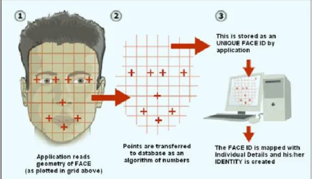
A representation of the means for the face acknowledgment framework is given in Figure1.
Acquire Image Face Detection Face Recognition Detected Person
Figure 1: Face Recognition System A. Acquire Image
In first step of Face recognition system, take an image from the camera and transfer it into the Computer. Because without an image no further processing is possible.
B. Face Detection
When the image is acquired from camera to computer and finally ready for mathematical computation using grabber as a first step in face detection. The input image is converted into a digital data and then forwarded for further processing. The first step after this is face detection which is done by some face detection algorithms. Many algorithms are available for this purpose. The available methods are further classified into sub units as Knowledge based and appearance based face detection. If we talk about very simple phenomena about knowledge based is the method which is derived from human knowledge for features that make a face. Similarly, appearance based method is derived from training or couching methods to learn to find face. However, as to detect a face for a human is easy but it is very hard for a computer to do the same job because it requires a lot of processing and perfect algorithms to perform such operations. For example to detect a face from an image, a computer may face cluster type issues which occur because of because of varying skin with age, facial expressions, and changing color. One more thing which makes it more difficult to identify the right image is saturation which includes change of light on the face, the different angle at which that picture is taken, geometry of shape, size, and background color saturation. Hence, an ideal face detector is the one which detects the face despite of the fact that face is facing color saturation issues, expression and varying geometry issues.
Figure 2: Knowledge Based Face Detection C. Face Recognition
Face recognition is a method in which the detected image is compared with trained dataset. When a face or faces are detected, the next step is to recognize them by comparing with some data base information. In literature, most of the methods are using image from the library and hence they are using a specific standard image. These standard images are created with some specific algorithm. From them the detected faces are send to face recognition algorithms. In literature, these methods are divided into 2D and 3D methods. In 2D method, a 2D image is taken and taken as input for processing. Some training methods are used for the classification of people. While in 3D method, a 3D image is taken as input and then different approaches are used for recognition. Using relative point measure, contour measure, and half face measure, these 3D images are recognized. However, like face detection face recognition also face some problems including, cluster issues, structural components, facial expressions, face orientation, condition of image and time taken for recognition. Some solutions are also available but they handle only one or two issues at a time. Therefore, those methods have many limitations for perfect face recognition. A robust face recognition system which is quite well for face recognition and gives error free output is a bit difficult to develop. To get easy understanding of recognition, a picture is shown below.
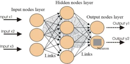
Figure 3: Introduction to Face Recognition D. Introduction to Neural Network
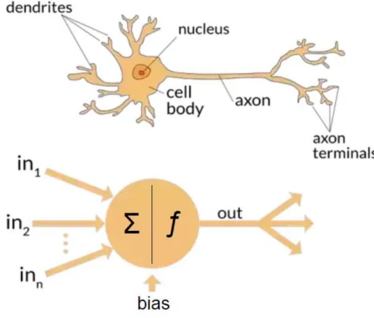
Neural network or artificial neural network is a computing system which is quite related to biological neural network, where numerous neurons work as messenger and transfer every kind of information within whole body of an organism. As neurons work in a way like if a person sees a picture having human faces, then eyes act as primary sensors just like input part and then brain complete the programming to identify whether that face is a known one, all middle work is done through these neurons. In the same way computing neural network works. It depends on the training of a system in its initial phases. Then such systems learn to perform given tasks by setting the training. Generally this is done through programming and one of best understanding of this system is recognition system. For example, in image recognition such system either learn whether the given image is labelled or unlabeled. Assume there is a cat in an image then such system will depend on its face, eyes, ears, tail, fur etc. in order to identify the respective target. Thus, once such systems are trained then they easily detect that cat with taking quite less processing time. A NN is a collection of different sub-units and the work is done by neurons. Each neuron is connected with another one and make a chain. This chain is like a synapses which can transmit and receive vital information. Even in artificial system neurons have ability to process the information as per capability and then forward it to neural network. In short in a neural network,
the signal is divided into two main parts, input and output. Input is a real number while output is calculated by some non-linear functions of input summation. The connection of neurons in signal transmission is known as edges. Typically, neurons and edges have some wait and all hidden layers with bunch of neurons make a whole system basing of weight information. However, this weight is adjusted by training the system as per need. In case of weight increases or decreases, the signal connection strength increases or decreases.
Neural network has many applications in daily life usage, including human face detection, artificial intelligence for robotics, in medical diagnosis, in speech recognition system, in video games etc. Neural network is shown in detail in pictures below,
Figure 5: Functional and Biological ANN E. Statement of the Problem
The main problem of thesis is to design such a unique face recognition system which can easily detect and recognize the face and can prove itself a worthy application for robotics as main vision and in the field of mechatronics. This project will detect and recognize the live image and will be useful in robotics and army surveillance cameras and as office robot. Later this project can be extended in drones to meet latest possible solutions.
F. Scope of Thesis
This face detection and recognition system will timely detect and recognize the face from image
This system will work under various color saturation issues This system will be able to detect multiple faces from one image
G. Outline of Thesis
Second chapter will explain about previous methods and their detailed work under literature review section.
Third chapter is about methodology and will describe the method and techniques which are introduced in this thesis.
Fourth chapter is about the whole summary of thesis and results taken from Eigen face detection and deep neural network algorithms.
Fifth chapter is about final discussion and it concludes the thesis. Chapter 5 discusses and concludes thesis.
II. LITERATURE REVIEW
A. Review
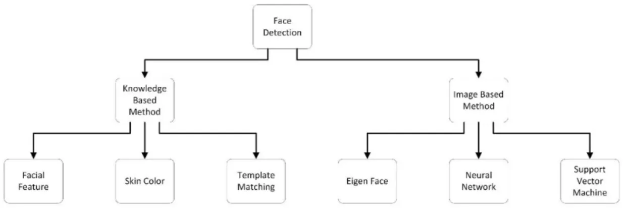
Face recognition is well known technique for many years. Many researchers are working on face recognition and its advanced level. The main difference between face recognition and face detection is, the face recognition actually concerned only with the recognition of face by comparing it with some previous data saved either in database or with training data. For this purpose many algorithms with increasing accuracy remained in use. The basic idea behind using such algorithms is to identify the face just in case to find whether the person being monitored is a criminal or not, similarly, for security purposes, for login details, and sometimes as an alternative to other biometric identifiers. Well, recognition comes after face detection. Face detection is different from face recognition and it only deals whether the image is provided as an input has any face or not. It also uses some algorithms to find out the location of face within an image. As the name is so easy to get this idea that what it means and why it is used but its implementation is not that easy as its name. It faces many issues while classification process. Hence, the word face recognition is kind of different thing than face detection. To recognize a face after detection, some previous used techniques are divided into following parts,
Detection of Target Recognition of Target
Detection & Recognition of Target B. Detection of Target
Face recognition includes face detection as a first step in order to find the face or faces from the whole picture. That face is detected initially on the basis of face features like nose, eyes, mouth etc. Detection techniques used and discussed in literature are quite tough to classify because most of the algorithms are based on how to increase the efficiency and accuracy of face detection. Here, two methods are
discussed including Knowledge based and picture based. The detection picture using these methods is shown below in figure.
Figure 6: Detection Methods
While discussing in detail, Knowledge Based techniques use information regarding face features and color matching. Further, the face features are useful in finding location of eyes, nose and mouth, and some other facial expressions in order to detect face. Color changing techniques are useful in selecting a specific area which indicates different styles of body posture and most importantly its characteristics do not change with varying color combinations. However, Skin color is divided into further color schemes including RGB, YCbCr, HSV, YUV, and statistical models. As face has different characteristics than other objects so on the basis of such color schemes face is easily differentiated from other objects and thus, it is easy to scan for a face from an image.
Face features play a vital part to provide standard information about the detection of a face. In literature review there are different methods available to simply detect and extract the optimum information about the detection of a face. These methods are explained below in detail.
1. YCbCr Method
Some researchers including Zhi-fang et al (Zhi-fang, Zhi-sheng, & Jain, 2003, p. 3). Who detected faces and facial features by excluding different regions of skin including YCbCr color schemes and in this technique, the edges of face features are detected. Hence, by using this technique only sharp color based edges of different face features are extracted. The next step is to find eyes, to do this he used PCA (principal Component Analysis) on the pre-processed sharp edges. Now, sharp edges and eyes are found, the next step is to find the mouth and to do so, geometrical information is used which caters the angle and distances of all features from one another and then on the basis of their angle and specific distance, location of mouth and some other features are extracted. These features are extracted only using one technique known as YCbCr. Flow of Algorithm shown n below Figure.
Figure 8: Flow Chart of Face Recognition using Color Image Feature Extraction 2. Face Detection by Color and Multilayer Feedforward Neural Network Method
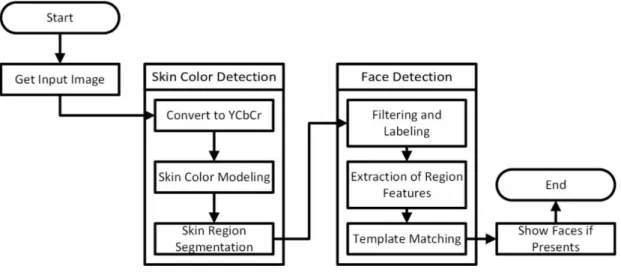
There is another approach, which extracts skin like regions by using RGB (red green blue) color space and in this method only RGB based color regions are detected and finally the whole face is verified by their template matching process which is done by RGB pre-processed image (Lin, 2005, p. 2).
Figure 9: Flow Chart of Face Detection by Color and Multilayer Feedforward Neural Network
3. SVM Method
Another researcher Ruan and Yin (Zhao, Sun and Xu, 2009: 5-6) segmented skin portions in YCbCr space and besides using PCA to find eyes and etc. He preferred SVM (support vector machine) to detect faces. As it is just an initial phase so for final face detection and verification through this process, like to find exact eyes, nose, and mouth already extracted information about Cb and Cr is used and by finding their differences the location of eyes, nose, and mouth is determined and thus, the face is detected. However, for finding eye region, Cb value is larger than Cr value and for mouth region value is vice versa.
Figure 10: SVM Method Flow Chart 4. Statistical Method
There is another approach (Zhao, Sun and Xu, 2006: 4-5) to detect face by using the same Cb and Cr values with a little change in selection and implementation phase. The first step in this technique is the separation of skin regions in to mini segments and this is done by using some sort of statistical model. Such statistical model is
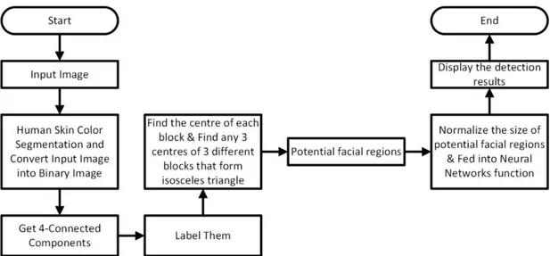
detected using selection of rectangular ratio of segmented regions. However, eyes, nose and mouth are verified by using segmented map of whole face. Here RGB color vector is also useful in making segments of skin. In case of segments made by RGB, the face is detected on the basis of face features distances by using isosceles triangulation of eyes, nose, and mouth. In this way, in the end a face s detected because distance between eyes to mouth is same as it is drawn by isosceles triangles which means a triangle is taken from eyes to mouth by taking nose as a mid-point.
Figure 11: Flow Chart of Statistical Method 5. FFNN Method
After statistical method, for final face verification FFNN (feedforward neural network) is used. According to Bebar et al. (M. A. Berbar, H. M. Kelash and A. A. Kandeel, 2006: 5) segments made with YCbCr color space and face features on the summation of segments and edges. After then, image is taken as horizontally and vertically. This horizontal and vertical position of image is used for final verification too. In previous mentioned methods, one can easily pick the concept that almost all methods are using skin segmentation in order to pick only facial parts.
Figure 12: FFNN Method 6. Gaussian Distribution Model
One of most prominent feature of face is its skin color, which makes a big difference while in detecting the face, and as everyone has different skin color. Some methods like parameterization/no-parametrization can be used to model the skin color for respective task. So by setting some threshold for skin in color differentiation, it is quite easy to identify the right skin according to the job. As some methods are being used for detection and one is RGB and other are YCbCr, HSV. The flaw in using one of these schemes is that RGB is sensitive to light changes while other YCbCr and HSV are independent of this issue. The reason why these two are independent of light changes is that these two methods use their own color channels where RGB only depends on mainly three colors. As already mentioned in literature there are many
Some other researchers, Kherchaoui and Houacine (S. Kherchaoui and A. Houacine, 2010: p.2) also used skin color technique by using Gaussian Distribution Model with YCbCr parameters involving Cb and Cr. After this, a specific bounding box is chosen as origin and on such basis target face is verified by matching with different templates. One another and easy way to this technique is the preprocessing of image where background of image is already removed and then it is further processed and background removal is done by applying some sort of edge detection on components of CYbCr method. After then, the selected region is filled up for part. As the image at this step is already filtered from background and further focused on a specific part so the next step here is segmentation which is done by some previous used and discussed methods. Then, the segmented portions are taken as pre-final face verification and for this purpose, entropy of that processed image is calculated and compared with the threshold and finally taken as verified detected face (Huang et al., 2010: 8).
Figure 13: Gaussian distribution Model 7. White Balance Model
Qiang-rong and Hua-lan (2010) also contributed their vital part in face detection by using white balance correction in preprocessing. The reason to use this step is because the image is often goes under different color saturations and thus it effects the performance in detection, to overcome this issue white balance is applied in initial stage of image where this color saturation issue is removed. After this step those region rich in color are segmented using elliptical model while remaining in YCbCr method. Once the skin portions are found, then they are merged with the sharped edges for
converting the image into grey scale. In final stages, the mixed regions are checked by using the same bounding box ratio analysis and area inside the box.
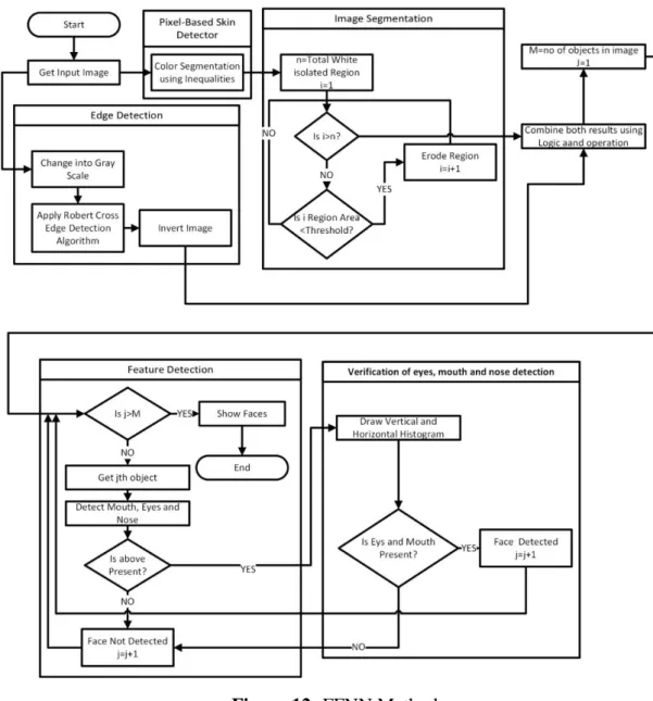
Figure 14: Flow Hart of White Balance Approach 8. AdaBoosting Method
There is one more method through which segmentation is done and parameter like Cb and Cr are found, then theses parameters are normalized and r and g new parameters are stored. Now face is chosen w.r.t bounding box and minimum area of region is selected. Now, when the exact target face is detected then AdaBoosting method is used further to clarify the target face. The final verification is completed by merging the results of skin portions with AdaBoosting (Li, Xue and Tan, 2010: 6).
Figure 15: Flow Chart of Face Detection Using AdaBoosting Method
As the skin color can also be changed by using some para-elliptical portions of calculated Cb and Cr parameters. Now, the skin portion is only segmented when there is any color inside the elliptic region and then those regions are verified by applying changing templates (Peer, Kovac and Solina, 2010: 9). Another researcher Peer et al. (Peer, Kovac, & Solina, 2003, p. 5) detected target faces by applying only skin segmentation and generated skin color characteristics under RGB bands. There is one more technique widely used in literature and that one is Self-Organizing Map (SOM) and Neural Network (NN) (Kun, Hong and Ying-jie, 2006: 6).
9. Scanning Method
One most prominent feature, which makes a human face easy target for detection, is its pattern of shape. So applying template is kind of easy way on the segmented data or scanned image. However, in case of using scanning method a small window of roughly 20x30p pixel window is selected. This method verifies all parts of original image and then it automatically decreases the image size in order to maintain re-scan on the image for better results. Here, as image size is decrease that is very important to locate small, medium and large face parts. However, this process is timelier as it needs to manage some computational work. While, template-matching need less processing time than scanning, because it only caters matched segments. Still there are many template-matching techniques available in literature.
10. Face Detection Based on Half-Face Template
One of researcher used some template techniques. Chen et al. (2009: 8) used template matching method and he chose half-face instead of full-face. The reason to choose this half-face method is that it decreases much computational time. Further, this method can be easily used in face orientations.
11. Face Detection Based on Abstract Template
Here one more template matching technique (Guo, Yu and Jia, 2010: 7) is available which is known as abstract template and this is not based on image while it is sum-up size, shape, color and position. Here still segmentation is done through the same old method of YCbCr. After segmentation eyes pair of abstract template id applied on it, here there are two parts of this template, the first one locates eyes while the second one locates the each eye. However, second template also capable of determining eyes orientation.
Figure 16: Flow Chart of Abstract Method Based Face Detection
After this image based methods come into words and these methods help in the comparison of face and no faced image. For such methods, large number of images of faces are no faces are used to train the network. Here, AdaBoost, Eigen, support vector machine and Neural Network come into place. In Adaboost method, a new term is introduced for face and no face images known as wavelet. Before apply any of such method, PCA and Eigen is used to create feature vector of faced and no faced image. One positive point of PCA is that is also compresses the feature vector and thus it becomes less time consuming. However, like wavelet, another term known as Kernel function is used in support vector machine to do the almost same job. Then face and
AdaBoost is the only algorithm which is enough capable to strengthen the weak classifiers. To move on with this method, the first step face detection is made by AdaBoost and then for its verification second series classifier is used. This algorithm is capable of handling +-45 left, right and front pose (Bayhan and Gökmen, 2008). 12. Face Detection Based on Template Matching and 2DPCA Algorithm
As mentioned previously that PCA is used for generating feature vector in Eigen faces method. However, window scanning can also be used in this method instead of PCA. Similarly, Wang and Yang (2008) applied geometric template to match the target face. 2D PCA is utilized to extricate the component vector. The picture lattice is legitimately given to the 2D PCA rather than vector. That diminishes computational time for figuring covariance grid. After PCA is connected, Minimal Distance Classifier is utilized to order the PCA information for face or non-face cases.
Figure 17: Algorithm of Face Detection Based on Template Matching and 2DPCA Algorithm
Another approach utilizes PCA and NN. PCA is connected to the offered picture to extricate the face applicants from the outset. At that point, up-and-comer pictures are characterized with NN to dispose of non-face pictures (Tsai et al., 2006).
Figure 18: Algorithm of Face Detection Using Eigen face and Neural Network Additionally, PCA and AdaBoost applications are connected with window examining method. First PCA is connected, that resultant component vector is utilized to contribution of AdaBoost strategy (Mohan & Sudha, 2009, p. 2).
For last technique for picture, based methodology is the Support Vector Machines (SVM). SVM is prepared with face and non-face pictures to develop a bit capacity that order the face and non-face pictures. A portion of the execution of SVM is distributed in (Wang et al., 2002: 3). A Different methodology is connected to discover face applicants in. The face competitor is found by summed up symmetry dependent on the area of eyes. At last, face applicant is approved/characterized with SVM. Additionally, SVM can be connected to distinguish faces with checking method. Jee et al. (2004, p. 5) apply skin like district division dependent on YCbCr and eye competitor are found with edge data inside the area. At that point, eyes are confirmed utilizing SVM. After check, face up-and-comer are removed concerning eye position. As a last confirmation, face applicant is sent to SVM for check.
Another methodology for SVM is utilizing one class based SVM. Rather than creating two classes that are face and non-face, just face class is produced. Since, it is hard to demonstrate the non-face pictures (Jin, Liu and Lu, 2004).
C. Recognition of Target
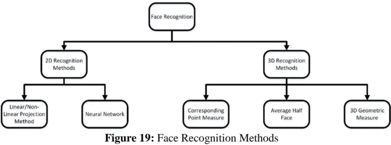
For face acknowledgment framework, the other part is acknowledgment part. The acknowledgment can be accomplished with 2D or 3D picture information, the two of them have focal points and impediments. 2D picture information can be gotten effectively and more affordable than 3D. Then again, 2D pictures are touchy to light changes however 3D pictures are most certainly not. With 3D pictures, surface of the face can without much of a stretch displayed however 2D picture does not contain the profundity information. Additionally, face acknowledgment calculations are performed over the face libraries. These libraries are made with standard face pictures, so the face acknowledgment framework should manage this issue. The techniques for face acknowledgment are given in Figure 19. Face acknowledgment is an example acknowledgment issue, so preparing/learning calculation ought to be utilized to make examination between the appearances. For 2D acknowledgment, Straight/Nonlinear Projection strategies and Neural Systems are utilized. Straight/Nonlinear Projection strategies are PCA, Direct Discriminant Investigation (LDA), Gabor Wavelet, and Otherworldly Element Examination. Neural System methodologies are Wavelet NN, and Multi-Layer Bunch NN. For 3D acknowledgment application, Comparing Point Measure, Normal Half Face and 3D Geometric Measure are utilized. 2D Direct/Nonlinear Projection strategies create include vector for every individual, at that point arrange the information individual inside the database. Producing highlight vector likewise has significance to lessen measurement of the information pictures.
Figure 19: Face Recognition Methods
1. Face Recognition Based on Image Enhancement and Gabor Features
One methodology applies picture upgrade to smother the awful lighting condition before acknowledgment process. Picture upgrades are known as logarithm change and standardization. At that point, highlight extraction is finished with Gabor
Wavelets. At last, utilizing Fisher Face, input face is grouped (Wang and Ou, 2006: 3). Song et al. (Song, Kim, Chang, & B. Kwon, 2006, p. 4) apply an alternate methodology on picture preprocessing/upgrade. For preprocessing before highlight extraction, ascertains the enlightenment contrast among right and left piece of face. In the event that there is a lot of distinction than take the reflection of normal enlightened part. After face picture is preprocessed, highlight extraction is finished with PCA.
Figure 20: Algorithm of Face Recognition based on Image Enhancement and Gabor Features
2. Layered Linear Discriminant Analysis Method
Characterization of highlight vector is finished with Euclidian Separation. Other execution uses Layered Linear Discriminant Analysis (LDA) to characterize faces, and the advantage of Layered LDA is utilizing little example size database.
In this method (Razzak et al., 2010: 5), the main difference that makes this method unique from others is computation of features vector and then comparing those with trained one and with input data and then recognition, results are shown. So starting from the training, like others dataset is taken for training purpose and proceeded ahead where features of all images one by one extracted. Once feature of an image is extracted then by using those feature a subspace feature vector is generated. This vector is responsible for matching faces in later step. However, one by one all feature vectors are generated for all training data and network boosts up for testing. An input image is taken for the testing phase and applying the same approach, its features extracted in very first step, then by using those features a feature vector is generated like training data. Now, this feature vector is compared with the trained network feature vectors one by one. In any case where feature vector matches with the trained network feature vector then output is generated with a recognized face. Otherwise, no output is generated and a new image is loaded for the same purpose and
thus, network works on its own. Being short in process is okay but still this network lags and has some issues.
Figure 21: Face Recognition using Layered Linear Discriminant Analysis Additionally, utilizing Ghostly Component Investigation can lessen the example size in database. Expanding the element extraction can improve the presentation of the framework for example applying Gabor wavelet, PCA and after that, Independent Component Analysis (ICA) on face picture. After include extraction is connected, at that point cosine comparability measures and the closest neighbor characterization guideline is utilized to perceive (Liu and Wechsler, 2003: 3).
Figure 22: Independent Component Analysis 3. PCA Method
Another methodology (Meena and Sharan, 2016: 4) for information vector utilizes facial separation. Measurement decrease is performed with PCA and characterization is accomplished with NN.
In PCA method, the main difference from other methods is use of Covariance matrix, mean and Eigen faces approach for face recognition. However, first of all input
data is loaded for training purpose and one by one covariance matrix is calculated for each image and this process continues till covariance matrix of all training images are calculated. After calculating covariance matrix the mean value is also calculated for each image and the process is proceeded to Eigen space where Eigen values and Eigen vectors are generated from the covariance and mean matrix. When this process does all images, it means training of this network is completed and is ready to test. When a test image is applied then like training images, its mean is calculated in a very first step. Once mean is calculated, then it is centered into the centered image and next step Eigen space is activated. At this point again, its Eigen values and Eigen vectors are calculated and finally this Eigen value and vector is compared with the previous calculated trained network Eigen values and vectors. In a case when covariance is positive then output image is shown and face is recognized as Eigen space matches, otherwise no output is detected and new image is loaded for testing.
Figure 23: Face Recognition using PCA 4. LBP Method
In LBP method (Olivares-Mercado et al., 2017: 4), first for training image is chosen from the database and then loaded to LBP where 3x3 filter is applied on it before any further proceeding. Once image is converted into 3x3 filter then feature extraction and concentration phase is activated where features are extracted of the object and all images from dataset passes through the same phase. When all dataset is trained then testing of image is activated where, an input image is given to the system and face detection checks the face from the target image, in case if there is no face detected then process ended and new image is loaded. Otherwise, that detected face
passes through a 3x3 LBP filter and after conversion it goes for classification phase where face is compared with the trained network. If any face matches from the training data, then face is recognized and output is generated otherwise no output is shown and new image is loaded. Hence, any image is checked by using LBP method. There is no doubt that this method is a small one but this method has some issues.
Figure 24: Face Recognition using LBP Method 5. Wavelet NN
Wavelet NN uses move work, which is produced using wavelet work arrangement, and this arrangement maintains a strategic distance from the visual deficiency in structure plan of BPNN. Then again, rather than utilizing grayscale pictures, shading pictures can be utilized as contribution to the BPNN (Youyi and Xiao, 2010: 3). R, G, B channels are inputs together What’s more, organize feed with shading data for simple segregation (Youssef and Woo, 2007: 4). Analysts additionally take a shot at consequences for utilizing distinctive sort of systems and highlight extractors. As system, BPNN, RBNN, and Multilayer Group NN utilized and as highlight extractor, Discrete Wavelet Change, Discrete Radon Change, DCT, and PCA (Rizk and Taha, 2002: 4). The best execution is accounted for as the blend of BPNN with DCT.
Rida and Dr BoukelifAoued (2004, p. 3) actualize FFNN with Log Sigmoid exchange capacity system to group the given appearances. Quick ICA utilized as highlight extractor and RBNN utilized as classifier (Mu-chun, 2008, p. 3), and just RBNN is utilized to characterize the info pictures (Wang, 2008, p. 4). Likewise, Particular worth Decay (SVD) is utilized as highlight extractor in BPNN (Rasied et al., 2005 p. 3). Another kind of picture improvement application is utilizing the Laplacian of Gaussian channel, at that point applying SVD to separated picture to get the component vector. At long last, face picture is grouped by utilizing FFNN (Pritha, Savitha and Shylaja, 2010).
6. 3D Recognition Method
3D face acknowledgment strategies utilize 3D information of face, which is made out of haze of focuses. One usage utilizes iterative nearest point to adjust face. At that point, as picture improvement, commotions are diminished and spikes are evacuated. The nose tip identified and a circle is trimmed with beginning of nose tip. This circle is highlight of the face. At that point, utilizing Comparing Point Heading Measure the given face is grouped (Wang, Ruan and Ming, 2010). Various methodologies utilize half face rather than full face. The normal half face is created with Symmetry Saving SVD. At that point, highlight extraction is finished with PCA and characterization is accomplished with Closest Neighbor Grouping (Harguess, Gupta and Aggarwal, 2008, p. 4). Elyan and Ugail (2009, p. 8) connected contribution as facial profiles. Focal Symmetry Profile and Cheek Profile are separated for countenances and Fourier Coefficients are found to produce highlight extraction. At last, Closeness Measure is connected to group the appearances. The geometric data about facial highlights is utilized in (Song, Wang and Chen, 2009, p. 3). Nose, eyes and mouth are found and 3D geometric estimations are connected. The estimations are straight-line Euclidean separation, shape separation, region, edge, and volume. The arrangement depends on Similitude Measure.
III. METHODOLOGY
A. Introduction to Purposed Solution
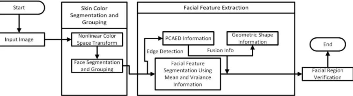
In previous chapter different techniques, algorithms, systems and combination of these techniques from different research papers are discussed which are used to detect face from image and recognize person. Every technique have some advantages but also have some disadvantages. In this thesis, the purposed solution to face detection and recognition is done by two main methods including Convolutional neural network and by using Eigen Faces. Here, convolutional neural network is used for face detection and Eigen Faces method is used for face recognition purpose. First of all the training data is taken from an online source named as Caltech 101 database and then train the classification layers of pre-trained image classification Deep Neural Network. After that, detected face is taken out for recognition and further Eigen faces method is used for face recognition. Eigen Faces loads the ORL dataset and applies algorithms on it and on the basis of features extraction and the detected face is recognized. The whole Project is implemented in MATLAB. Flow chart for proposed solution is shown in below figure,
B. Input Image
The prerequisite for face recognition system is input Image. In this part, Image acquisition operation is performed. After loading image from directory or capturing image Live, Acquire image is sent to Face Detection Module.
C. Face Detection
Face Detection Algorithm find either input image have any face or not. Deep Neural Network is used to detect face image. If we build Deep Neural Network from scratch, we required a large amount of training data that’s also take huge bundle of time for training. Therefore, we choose Pre-Trained Neural Network instead of build Neural Network from scratch. Pre-trained image classification network has already trained to extract features from images. It is used to train a new network with small no of training dataset. It saves a lot of time because its weights are already optimized. Due to optimization, it converges fast. In this project Resnet50 pre-trained Neural Network is used for face detection (detail about this is explained in below Topics).
First train classifier of the Resnet50 from scratch, which required dataset. Therefore, we used four categories (Faces, Airplanes, Ferry, and Laptops) of Caltech 101 dataset to train classifier. Caltech 101 is in general form. Therefore, there is no need to crop. As data from Caltech 101 database is labelled already so, there is no need of any kind of annotation before applying to Resnet50. Training Dataset detail shown in Table no. Resnet50 input layers accept image having size 224-by-224-by-3. So first we adjust size of all training images same as input layer size. Here are some samples of training dataset shows in figure.
Figure 26: Training Dataset Samples Table 1: Training Dataset Samples
Category Name
No of Images for Training
Faces 435
Air Planes 800
Ferry 66
Laptops 81
After training, we saved updated Resnet50 Model. In order to test trained model, we loaded image from directory and change size to 224x224x3. Then pass through Resnet50 updated model. Resnet50 Model output returns Label of category which maximum features presents in input image. If input image belong to faces category, then it will be send to Face Recognition Algorithm to identify face. In case if there is no face detected by comparing with the pre trained data then it directly ends the current algorithm and starts the next round and keeps on doing till all data is accessed and classified. Output of face detection shows in below Figure.
Figure 27: Output of Face Detection Part Flow chart of Face Detection Method given in below figure.
Figure 28: Flow Chart for Detection Purposed D. Caltech 101 Database
Caltech 101 database is an online database which provides various kind of data for different purposes. This data is used for image detection, recognition, and for visual computations. Most of dataset is used in image training and computer visual algorithms. Images in dataset are saved in a way to avoid any sort of cropping, reshaping, and clutter. However, Caltech 101 is working to resolve some common issues which are as follows,
Reshaping of images.
Single and multiple class compatibility. Numerous outline of different objects. General operations to use different datasets.
However, according to a recent study there are still some issues with Caltech 101 datasets which causes misleading results.
1. Images
Caltech 101 dataset contain a vast set of different dataset classes. However, current situation indicates that Caltech 101 dataset contains about 9150 images and further these images are divided into different categories including background cluttering. Each set of different category is further classified into similar data with images ranging from 40 to 800. However, common and most used classes contain more images than the standard range. Each image in the dataset has about 300x200 pixels witch is quite enough to compete training sort of issues. Images oriented in airplanes and similar class is shifted from left to right orientation and building are shifted vertically.
2. Annotations
For easiness each image is marked with detailed set of annotations. Each class is further divided into two different categories based on their information. The first one is known as general box which holds the location of image, and the second one is detailed outline for human specification and for easy access for a machine too. Along with such annotation a well-known coding software Matlab script is also presented which gives a benefit of producing Matlab figures without any complex work other than just loading that scripted image from Caltech 101 dataset directory.
3. Uses
Caltech 101 dataset has many uses as shortly explained in introduction. It has a vital role in providing datasets for training networks, for computer vision recognition, and for many other purposes including classification algorithms. Some main uses are as follows;
Pyramid match kernel which basis on classification of images on the basis of features.
Combination of Generative models with fisher kernel. Visual cortex use for object features based recognition. Discriminative neighbor classification.
For nature based images recognition use of spatial pyramid. Multiclass filters for different type of object recognition. Multiclass localized feature based recognition.
Classification in generative framework. 4. Advantages
There exist some advantages of using this online dataset provider which are as follows;
Unique size for every class. Already cropped image. Low level of clutter.
Effective background comparison with target object. Explained marked outline for each image in every class. 5. Disadvantages
Where there exist a lot of benefits of using this online dataset provider, there exist some disadvantages too which may cause faulty results;
Extra clean dataset which causes reality based classification issues. Uniform shape causes unrealistic results.
Limited number of categories.
Less images than standard in some categories which causes wrong training. Aliasing issues because of changing orientations.
E. Resnet50
First of all, a pre trained network is a network which contains already a specific set of weights and biases of different objects features. Later on the basis of such dataset training is made. One basic example is, assume there are a number of birds and one
needs to identify a specific one then by using such trained network he can easily detect by providing his input to the already trained network on animal class. Restnet50 is one of the pre trained network. Resnet50 is a neural network which is already trained with more than millions of images of different categories. This network has many layers up to 50 which classifies more than 1000 images including different categories as car, animals, daily usage accessories, laptops, nature, and many more. So in the end it is quite clear that this network is trained with rich features and with wide range of images of different categories. As deep neural network is difficult to train itself so, rushing towards resnet50 is a good option as it provides many benefits and one just need to pass an input image through this network and no need to design any nodes or layers or filters because everything is already set at a standard. However, resnet50 also provides access to classification layers to alter them according to the requirement. In this way, we can become so controllable over our network to ensure that output is according to the need. Simple is we can easily reformulate the layers for training purpose rather than using deep neural network and designing every filter and layer on its own is a difficult task with poor output. However, by using this already train network, we can easily optimize our algorithm for desired accuracy. As discussed above, resnet50 has taken datasets from different online dataset provider site including ImageNet and Caltech 101. In ImageNet resnet50 uses 150 round about layer with 8x resolution over VGG Net and still it goes with less complexity. In error format, while using ImageNet about 3.8% error appears which is quite less than other classifications like ILSVRC. Similarly, Caltech 101 also provides optimized dataset which causes the resnet50 with less error over ImageNet and others. Thus, this network is so adoptable for many visual recognition tasks.
1. Resnet50 Layers
Resnet50 is just like another deep neural network with all layers and nodes etc. as above mentioned about 50 different layers of resnet50 are enough to classify the images ranging from 100 to 1000. Below image is showing all Relu functions, maxpool layers, classification layers and softmax layers.
Figure 30: Resnet50 layers 2. Layers Description
Table 2: Layers Description used in Resnet50
Layers
Description
Input Layers
Image 3D Input Layer Get three dimensional image as input and normalize him.
Convolution and Fully Connected Layers Convolution 3D Layer
Apply three Dimensional convolutional layer applies sliding cuboidal
convolution filters to three-dimensional input.
Fully Connected Layer It multiplies the input by a weight matrix and then adds a bias vector. Activation Layers
Relu Layer A ReLU layer set values to zero that’s are less than threshold.
Table 2 (con.): Layers Description used in Resnet50
Layers
Description
Normalization, Dropout, and Cropping Layers
Batch Normalization Layer A batch normalization layer reduce the sensitivity to network initialization by normalizes each input channel across a mini-batch. It is used to increase training speed of CNN.
Pooling and Unpooling Layers
Max Pooling 3d Layer A three dimensional max pooling layer performs reduces the no of samples by dividing three-dimensional input into cuboidal pooling regions, and
computing the maximum of each region.
Output Layers
Softmax Layer Apply softmax function to the input Classification layers.
Classification Layer A classification layer computes the cross entropy loss for multi-class classification problems with mutually exclusive classes.
3. Resnet50 Architecture
4. Resnet50 Tables Table 3: Resnet50 Layers
F. Face Recognition
For face Recognition, we required datasets contains multiple images of different persons. Therefore, we get online dataset of faces ORL. It contains images of 40 different persons, ten different images of every person. Images were taken at different light intensity, different facial expressions (for example open and close eyes, smiling and no smiling). The size of every gray scale image is 92-by-112 pixels. ORL dataset information shows in below Table also some samples are shown in below figure.
.
Table 4: ORL Dataset Information
Person Total Samples
10 10 10 10 10 . . . . . . 10
Total Persons: 40 Total Samples: 400
Face recognition algorithm first select one random image from all 400 images, which is used to for recognition. After that, calculate mean of remaining images. Load every remaining 399 images one by one and subtract mean from every image. Then create an array that contains Eigen vectors of every remaining Image. After that create matrix that contains Signatures of all remaining images. On the other side, after loading random image from database subtract mean of remaining images from random image and multiply Eigen vector (calculated above) with random updated image. Once updated random image is multiplied with the Eigen faces vector, calculate Signature
of input image of unknown person. After that, initialize N (Image no.) with one (mean image no. 1). After that, find difference between Signature of N=1 image and Random image Signature and store in every in variable “dif”. Then load Signature of every remaining image one by one and calculate its difference with Signature of Random Image. After that, find image having minimum Signature difference with Random image Signature. That image person is predicted as recognized face.
Output of Face Recognition Shows in below image.
Figure 34: Flow Chart of Face Recognition Algorithm G. Eigen Faces
Eigenfaces is the name given to a great deal of eigenvectors when they are used in the PC vision issue of human face affirmation. The approach of using Eigen faces for affirmation was made by Sirovich and Kirby and used by Matthew Turk and Alex Pentland in face portrayal. The eigenvectors are gotten from the covariance system of the probability dissemination over the high-dimensional vector space of face pictures.
The Eigen faces themselves structure a reason set of all photos used to build up the covariance lattice. This produces estimation decline by allowing the humbler course of action of reason pictures to address the first getting ready pictures. Request can be practiced by seeing how faces are addressed by the reason set. A great deal of Eigen countenances can be created by playing out a logical methodology called head fragment examination (PCA) on a colossal course of action of pictures outlining particular human appearances. Calmly, Eigen appearances can be seen as a great deal of "standardized face fixings", got from true examination of various photographs of faces. Any human face can be seen as a blend of these standard appearances. Strikingly, it doesn't take various eigenfaces combined to achieve a sensible estimation of by and large faces. In like manner, in light of the way that a person's face isn't recorded by a mechanized photograph, yet rather as just a summary of characteristics (one motivation for each eigenface in the database used), significantly less space is taken for each individual's face. The eigenfaces that are made will appear as light and diminish regions that are sorted out in a specific model. This model is the methods by which different features of a face are singled out to be surveyed and scored. There will be a guide to survey symmetry, paying little mind to whether there is any style of facial hair, where the hairline is, or an evaluation of the size of the nose or mouth. Distinctive eigenfaces have plans that are less simple to recognize, and the image of the eigenface may look beside no like a face. The technique used in making eigenfaces and using them for affirmation is also used outside of face affirmation: handwriting affirmation, lip scrutinizing, voice affirmation, correspondence by means of motions/hand signals interpretation and therapeutic imaging examination. As such, some don't use the term eigenface, yet need to use 'eigenimage'.
1. Practical Implementation
For Eigen faces following advances ought to be taken,
Prepare a readiness set of face pictures. The photographs building up the arrangement set should have been taken under a comparative lighting conditions, and ought to be institutionalized to have the eyes and mouths balanced over all photos. They ought to in like manner be all resampled to a common pixel objectives (r × c). Each image is treated as one vector, basically by interfacing the lines of pixels in the primary picture, achieving a lone section
with r × c parts. For this utilization, it is normal that all photos of the arrangement set are secured in a singular cross section T, where each area of the matrix is an image.
Subtract the mean. The ordinary picture an unquestionable requirement be resolved and a while later subtracted from each one of a kind picture in T. Calculate the eigenvectors and eigenvalues of the covariance arrange S. Each
eigenvector has a comparative dimensionality (number of portions) as the main pictures, and thus would itself have the option to be seen as an image. The eigenvectors of this covariance cross section are along these lines called eigenfaces. They are where the photos differentiate from the mean picture. Regularly this will be a computationally expensive development (if at all possible), anyway the conventional relevance of eigenfaces originates from the probability to process the eigenvectors of S gainfully, while never enlisting S explicitly, as point by point underneath.
Choose the essential parts. Sort the eigenvalues in diving demand and arrange eigenvectors as necessities be. The amount of head parts k is settled self-decisively by setting an edge ε on the full scale vacillation. Hard and fast vacillation, n = number of parts.
K is the most unobtrusive number that satisfies.
These eigenfaces would now have the option to be used to address both existing and new faces: we can broaden another (mean-subtracted) picture on the eigenfaces and thusly record how that new face contrasts from the mean face. The eigenvalues related with each eigenface address how much the photos in the arrangement set change from the mean picture toward that way. Information is lost by foreseeing the image on a subset of the eigenvectors, yet hardships are constrained by keeping those eigenfaces with the greatest eigenvalues. For instance, working with a 100 × 100 picture will convey 10,000 eigenvectors. In sensible applications, most faces can commonly be perceived using a projection on some place in the scope of 100 and 150 eigenfaces, with the objective that by far most of the 10,000 eigenvectors can be discarded.
2. Computing the Eigenvectors
Performing PCA legitimately on the covariance grid of the pictures is frequently computationally infeasible. On the off chance that little pictures are utilized, state 100 × 100 pixels, each picture is a point in a 10,000-dimensional space and the covariance network S is a framework of 10,000 × 10,000 = 108 components. Anyway the position of the covariance network is restricted by the quantity of preparing models: if there are N preparing models, there will be all things considered N − 1 eigenvectors with non-zero eigenvalues.
In the event that the quantity of preparing models is littler than the dimensionality of the pictures, the vital segments can be registered all the more effectively as pursues. Give T a chance to be the framework of preprocessed preparing models, where every section contains one mean-subtracted picture. The covariance grid would then be able to be processed as S = TTT and the eigenvector deterioration of S is given by.
Anyway TTT is a huge grid, and if rather we take the eigenvalue disintegration, at that point we see that by pre-increasing the two sides of the condition with T, we get;
Implying that, on the off chance that ui is an eigenvector of TTT, at that point vi = Tui is an eigenvector of S. On the off chance that we have a preparation set of 300 pictures of 100 × 100 pixels, the grid TTT is a 300 × 300 network, which is substantially more sensible than the 10,000 × 10,000 covariance framework. Notice anyway that the subsequent vectors vi are not standardized; if standardization is required it ought to be connected as an additional progression.
3. Facial Recognition
Facial acknowledgment was the inspiration for the making of eigenfaces. For this utilization, eigenfaces have points of interest over different procedures accessible, for example, the framework's speed and effectiveness. As eigenface is essentially a measurement decrease strategy, a framework can speak to numerous subjects with a moderately little arrangement of information. As a face-acknowledgment framework it is additionally genuinely invariant to huge decreases in picture estimating; be that as