Linear planning logic: An efficient language and theorem prover for robotic task planning

Linear Planning Logic: An Efficient Language and Theorem Prover for

Robotic Task Planning

Sitar Kortik

and Uluc Saranli

Abstract— In this paper, we introduce a novel logic language and theorem prover for robotic task planning. Our language, which we call Linear Planning Logic (LPL), is a fragment of linear logic whose resource-conscious semantics are well suited for reasoning with dynamic state, while its structure admits efficient theorem provers for automatic plan construction. LPL can be considered as an extension of Linear Hereditary Harrop Formulas (LHHF), whose careful design allows the minimiza-tion of nondeterminism in proof search, providing a sufficient basis for the design of linear logic programming languages such as Lolli. Our new language extends on the expressivity of LHHF, while keeping the resulting nondeterminism in proof search to a minimum for efficiency. This paper introduces the LPL language, presents the main ideas behind our theorem prover on a smaller fragment of this language and finally provides an experimental illustration of its operation on the problem of task planning for the hexapod robot RHex.

I. INTRODUCTION

As a result of rapid developments and decreased cost for mobile robotic systems, they promise to become more ubiquitous. From simple applications such as cleaning robots [1] to more sophisticated systems such as Mars rovers [2], mobile robots have been tasked with increasingly important roles. However, as these roles become more complex, the need for autonomy for robotic systems also increases. Even though teleoperation has been successfully used to overcome difficulties associated with operating a robot in remote and potentially hazardous environments [3], it suffers from in-herent problems in terms of its scalability and speed. Conse-quently, autonomy for mobile robotic platforms remains to be a difficult but important challenge.

Our work in this context focuses on task planning [4], which is the problem of finding a list of actions (plan) that can be used to reach a given goal in the presence of well-defined actions and resources. In general, each action is formally defined as having certain preconditions and effects, expressed in a suitable language. Preconditions must be satisfied using existing resources before an action can be used. If an admissible action is chosen for execution, the environment is modified with its effects, usually represented as new resources or facts. Plan search consists of finding a total or partial order of such actions, at the end of which the desired goal should be reached [5].

This general idea is not new [6] and has been instantiated in numerous different languages and methods. Among these,

1_{Sitar Kortik is with the Department of Computer Engineering, Bilkent}

University, 06800, Ankara, Turkey, sitar@cs.bilkent.edu.tr

1_{Uluc Saranli is with the Department of Computer Engineering,}

Middle East Technical University, 06800, Ankara, Turkey, saranli@ceng.metu.edu.tr

linear logic has been proposed in the literature as having sufficient expressivity to handle real-world planning prob-lems [7] as a result of its linearity, allowing native support for representing dynamic state as single-use (or consumable) resources [8], that are in stark contrast to fact representations in classical logic that can be used multiple times or not at all. As such, linear logic is capable of effectively addressing the well-known frame problem (the need and challenge of representing possibly irrelevant non-effects of an action in addition to its effects) that often occurs in embeddings of planning problems within logical formalisms [9, 10].

Unfortunately, the use of logical reasoning methods and theorem provers for practical domains such as task planning consistently runs into fundamental issues with computational complexity due to “extra” freedom in the multitude of valid proofs, resulting in nondeterminism beyond what is inherent in the problem domain itself, hence making the search problem much bigger [11]. Most research efforts to address this problem either focus on simplifying the representational language, or attempt to impose a particular structure on proof search without compromising the semantic soundness and completeness of the logic [12]. Our approach is a combination of both, providing increased expressivity relative to simpler but very efficient linear logic programming languages such as Lolli [13], while managing to keep the out-of-domain nondeterminism to a minimum.

To this end, we introduce a new language called Linear Planning Logic (LPL), which extends on Linear Hereditary Harrop formulas (LHHF) [13] that underlie linear logic programming languages such as Lolli. We propose a new proof theory for this language, preserving the deterministic back-chaining structure of provers designed for LHHF, while allowing negative occurrences of conjunction (representing multiple simultaneous preconditions for an action) that prove to be particularly problematic for linear logic. In order to keep the presentation clear and concise, we present our ideas in the context of a simplified language, mini-LPL, that pre-serves LPL’s critical features. We illustrate an experimental application of our new planning formalism on the problem of behavioral planning for a hexapod robot navigating in an environment populated with visual landmarks and show the feasibility of using LPL for task planning.

II. RELATEDWORK

Among most commonly known planning algorithms is Partial Order Planning (POP) [14], which introduced the idea of searching in the space of plans rather than the 2014 IEEE International Conference on Robotics & Automation (ICRA)

Hong Kong Convention and Exhibition Center May 31 - June 7, 2014. Hong Kong, China

larger space of orderings of individual actions. Substan-tial nondeterminism was eliminated by allowing plans to maintain a partial order between actions, focusing only on interactions that are relevant to the task at hand. An important variation was introduced by the Universal Conditional Partial Order Planner (UCPOP) method [15], which achieves greater expressivity by incorporating constraints as conditions on actions. UCPOP can encode actions that have variables, conditional effects, disjunctive preconditions and universal quantification. Despite their effectiveness, however, both the expressivity and the semantic completeness of these methods are impaired in the absence of formal foundations connecting them to a logical formalism.

A more recent practical alternative to these methods is GraphPlan [16], which proved to be faster than POP, albeit being less expressive. Even though both methods are based on the STRIPS [6] representation of states and actions, POP’s use of variables is more intuitive than GraphPlan which is restricted to propositional state components. This not only makes GraphPlan a more restrictive language, but also in-creases problem size when complex domains are represented within the framework. Some existing work addresses these problems by combining the expressivity of UCPOP with the efficiency of GraphPlan [17] by transforming domains in the former to their equivalent in the latter.

An alternative formalism for planning problems is Petri Nets, which has been used for assembly planning and task planning domains [18]. Assembly planning is finding a sequence of operations to assemble a product, for which Petri nets were first used by Zhang [19]. Transitions in Petri nets can be used to represent assembly operations and places to represent corresponding preconditions and results. Petri nets have also been used for robot task plan representation for modeling, analyzing and execution in [20] as well as semantic models for linear logic [21], through which research in this area is connected to our contributions as well.

Previous research has investigated different issues arising from the use of linear logic for planning. In [22], the authors argue that linear logic is appropriate for simple planning problems where actions can be either deterministic or nonde-terministic, having preconditions and effects represented as linear assumptions. In deterministic action definitions, there is only one possible set of effects. In contrast, disjunctive actions are nondeterministic since effects of an action may vary depending on the current state. In [23], the authors propose a new geometric characterization of actions and also translate conjunctive actions into plans. They define a pseudo-plan as a finite graph composed of vertices for actions and oriented edges for preconditions or effects of actions. In [24], the exponential search space problem in planning problems including functionally identical objects, such as identical balls in a box, was addressed, exploiting the resource conscious nature of linear logic. In [25], temporal concepts were incorporated into actions, allowing them to have quantitatively delayed effects. These studies focused more on the expressivity of the language and did not in-vestigate the efficiency of the planner, which is likely to be

intractable due to the explicit presence of the cut rule. Among recent studies considering the use of linear logic for planning is the implementation proposed in [26]. The proposed framework allows an action to interact with differ-ent agdiffer-ents through a dialogue, without requiring that agdiffer-ents share goals, plans and representations of the world. This allows implementation on a distributed architecture using the linear logic programming language Lolli [13] ported onto the distributed language Alice [27]. Our contributions in this paper focus on increasing expressivity, while preserving computational efficiency for planning languages based on linear logic.

III. LINEAR PLANNING LOGIC A. A Simple Robotic Planning Domain

RHex

camera landmark1 landmark2

landmark3

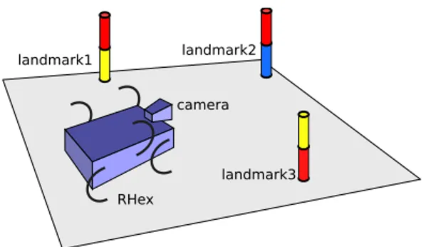
Fig. 1. An illustration of the simple planning domain including a six-legged robot equipped with a camera and three colored landmarks.

We begin our presentation by introducing a simple domain in which concepts and algorithms for Linear Planning Logic will be presented. The example domain consists of a mobile robot, the RHex hexapod [28] in this case, navigating in an environment populated with uniquely identifiable colored landmarks. Paths between each pair of landmarks can have surfaces with different traversability properties appropriate for different locomotory gaits of the robot. Moreover, the robot is assumed to have the capability of “tagging” land-marks, corresponding to a particular action carried out at that location. We capture this aspect of the domain with a persistent binary state, “tagged” or “untagged”, associated with each landmark. An illustration of this domain is shown in Fig. 1. For the sake of simplicity, our presentation in this paper except the last experimental example will only use two actions, Walk(X) and Tag(X), eliminating additional actions such as Run(X) for running on firmer ground towards land-mark X and Seek(X) for visually searching for landland-mark X. Predicate and action definitions to represent this simplified domain are summarized in Fig. 2.

An example planning problem in this domain, as we will show more formally in subsequent sections, would be tag a desired set of landmarks while leaving others untagged, using locomotory actions that are appropriate for paths traversed during navigation. We have chosen this relatively simple planning domain in order to ensure a clear presentation of our logical reasoning framework.

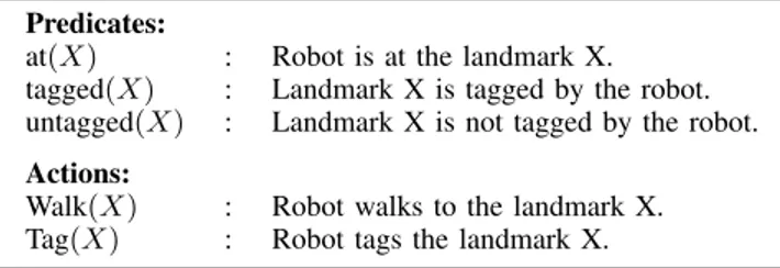
Predicates:

at(X) : Robot is at the landmark X. tagged(X) : Landmark X is tagged by the robot. untagged(X) : Landmark X is not tagged by the robot. Actions:

Walk(X) : Robot walks to the landmark X. Tag(X) : Robot tags the landmark X.

Fig. 2. Predicates and actions encoding the simple robotic planning domain.

B. Intuitionistic Linear Logic: Language and Proof Theory In logical reasoning, intuitionistic languages have the property that proofs have a close correspondence to exe-cutable programs as formalized by the Curry-Howard iso-morphism [29]. This motivates a direct application to plan-ning problems where a suitable encoding of the domain including its state components and actions, combined with representations of initial and goal states can be supplied to an automatic theorem prover to generate a feasible plan in the form of a proof. In this context, both the expressivity of the language, as well as the efficiency of the theorem prover are of critical importance since they directly influence the utility and feasibility of the framework. An unfortunate trade-off, however, is that the more expressive a logical language is, the less efficient associated theorem provers become due to the increase number of alternatives to consider (i.e. nondeterminism) at each step of the proof construction. In this context, linear logic, first introduced by Girard [8] and later received considerable attention in the literature, offers a promising combination of expressivity and efficiency in proof search for encodings of problems in need of model-ing dynamic state components. The linearity of the language restricts assumptions to be single-use, allowing a natural encoding of state components as consumable resources. This section presents a gentle introduction to most important con-nectives and their semantic properties within linear logic to support the theoretical foundations of our proposed method. For clarity, we limit our discussions to a smaller multi-plicative fragment of linear logic defined by the grammar

Program formulas: D ::= a | D1⊗ D2| G ( D

Goal formulas: G ::= a | G1⊗ G2| D ( G ,

where a denotes atomic formulae (e.g. the predicates sum-marized in Fig. 2). In the task planning domain, the simul-taneous conjunction connective (⊗) is used for composing resources or goals whereas the linear implication connective (_{() is used for relating preconditions to effects for actions.} We call this language mini-LPL since it captures all important aspects of the LPL to highlight our contributions.

Proof construction within logical languages is often for-malized within sequent calculus, which encodes consequence relations between provability statements in the form of inference rules. The first step in such formalizations is the definition of a sequent for a logical formalism that encodes the provability of a goal from a set of resources. For example, our sequent definition for a basic mini-LPL proof theory takes

the form

D1, D2, ..., Dn⇒ G , (1)

which indicates that the goal formula G is provable using consumable resources D1 through Dn, all of which must be

used exactly once. This last property is what distinguishes linear logic from others where assumptions persist indefi-nitely. ∆, α, β ⇒ G ∆, α ⊗ β ⇒ G ⊗L ∆1⇒ G1 ∆2⇒ G2 ∆1, ∆2⇒ G1⊗ G2 ⊗R

Fig. 3. Proof rules for simultaneous conjunction. The ⊗L rule on the left defines how a conjunctive assumption can be decomposed, while the ⊗R rule on the right shows how to achieve a conjunctive goal by decomposing available resources.

Sequent calculus formulations require “left” and “right” inference rules for each connective, encoding how reasoning should proceed for occurrences of that connective on the left or right side of the sequent, respectively. For example, Fig. 3 shows left and right sequent rules for simultaneous conjunction. Reading these rules from the bottom to the top, the resource conscious nature of linear logic is evidenced by the ⊗R rule, which requires that assumptions (resources) available on the left side of a sequent must be split into ∆1

and ∆2 between two subgoals G1 and G2. This is in stark

contrast to traditional logic systems where an assumption can be used as many times as desired. This property is also enforced by sequent rules associated with linear implication shown in Fig. 4, where the ( L splits available resources between the proof for the premise in the implication and its conclusion.

∆1⇒ α ∆2, β ⇒ G

∆1, ∆2, α ( β ⇒ G ( L

∆, α ⇒ G

∆ ⇒ α ( G ( R

Fig. 4. Proof rules for linear implication. The( L rule on the left first proves the premise, then proves the conclusion, splitting available resources as necessary. The( R rule attempts to prove the conclusion by adding the premise into available resources.

The proof system becomes completed by linking atomic assumptions to atomic goals using the init rule shown in Fig. 5. This rule occurs at the leaves of the upside-down proof tree whose nodes are instantiations of left and right sequent rules as shown in Fig. 9.

p ⇒ p init

Fig. 5. The init rule connecting atomic assumptions to atomic goals.

Based on the proof theory summarized above, we will now illustrate an important source of nondeterminism in proof search that is directly addressed by the method we propose in this paper. We first note that the construction of a sequent calculus proof proceeds recursively from the bottom

to the top, with the initial problem specified in the form of a sequent. For example, the following sequent might appear at an intermediate stage within our example domain:

at(b2) ⊗ tagged(b2) ⇒ tagged(b2) ⊗ at(b2) .

Even though the proof for this commutativity sequent is trivial for us humans to construct, an automated prover with access to only the sequent rules described above must consider all applicable alternatives, leading to substantial nondeterminism in the search.

?

at(b2), tagged(b2) ⇒ tagged(b2)

? at(b2) ⊗ tagged(b2) ⇒ tagged(b2)

⊗L ?

· ⇒ at(b2)

? at(b2) ⊗ tagged(b2) ⇒ tagged(b2) ⊗ at(b2)

⊗R

Fig. 6. Incorrect proof attempt using first the ⊗R rule, then the ⊗L rule.

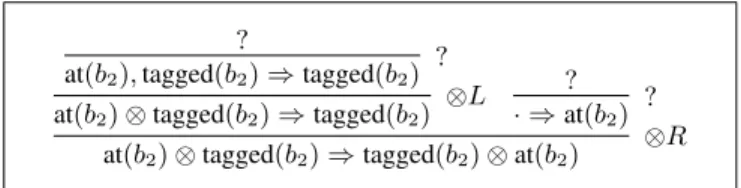
The first alternative we might consider would be to eagerly apply the ⊗R rule in reverse to decompose the goal into its subgoals. This is a strategy which is adopted by logic programming languages in general, with full decomposition of goals followed by back-chaining. The proof tree alter-native that results is shown in Fig. 6. Unfortunately, this eager decomposition of the goal does not lead to a valid proof in this case since the conjunctive goal on the left hand side must be assigned either to the first or the second goal, leaving the other one unprovable. The correct proof is given in Fig. 7. The availability of these two alternatives, combined with the combinatorial complexity of splitting resources is a significant source of nondeterminism in proof search.

at(b2) ⇒ at(b2)

init

tagged(b2) ⇒ tagged(b2)

init at(b2), tagged(b2) ⇒ at(b2) ⊗ tagged(b2)

⊗R at(b2) ⊗ tagged(b2) ⇒ at(b2) ⊗ tagged(b2)

⊗L

Fig. 7. Correct proof using the ⊗L rule first, then the ⊗R rule.

Fragments of linear logic that form the basis of linear logic programming languages address this issue by disallowing simultaneous conjunction on the left hand side of a sequent (i.e. negative occurrences) altogether [30, 31]. In such limited grammars, action representations become more complex, sometimes impossible [26]. Our solution is to use a novel resource management strategy to allow eager application of the ⊗R rule, keeping track of used and unused resources to effectively postpone the decision for splitting resources. C. Encoding the Planning Example within Linear Logic

We have already defined the vocabulary for our plan-ning domain in Fig. 2 in the form of predicates for state components and action labels. The next step is to associate these actions with mini-LPL expressions to formally define their preconditions and effects. Simple encodings for the Walk(X) and Tag(X) actions are given in Fig. 8, defined

parametrically on the landmark identifier X. Since mini-LPLleaves out universal quantification for simplicity, action instances needed for the proof will be manually instantiated but this is easily addressed by the full LPL language using unification methods. When using the Tag(X) action, if the robot is at an untagged landmark X, the robot tags X while remaining in the same position. Using the second action Walk(X) moves the robot from landmark Y to X.

Tag(X) : at(X) ⊗ untagged(X)( at(X) ⊗ tagged(X) Walk(X) : at(Y )( at(X)

Fig. 8. Encodings of walking and tagging actions within mini-LPL.

We now describe a simple scenario to illustrate the use of mini-LPL for task planning. Suppose we initially have two landmarks, b1 and b2, both untagged. The robot is initially

at b1 and the final desired position of the robot is b2 with

the property tagged(b2) asserted. Formally, the initial state

of the environment and the robot is given by the resource at(b1) ⊗ untagged(b2) ∈ ∆ ,

while the goal state can be encoded as G = at(b2) ⊗ tagged(b2) .

In order to satisfy the first subgoal, at(b2), the robot must

walk from its initial position to b2. For the second subgoal,

tagged(b2), the robot must use the Tag(b2) action to conclude

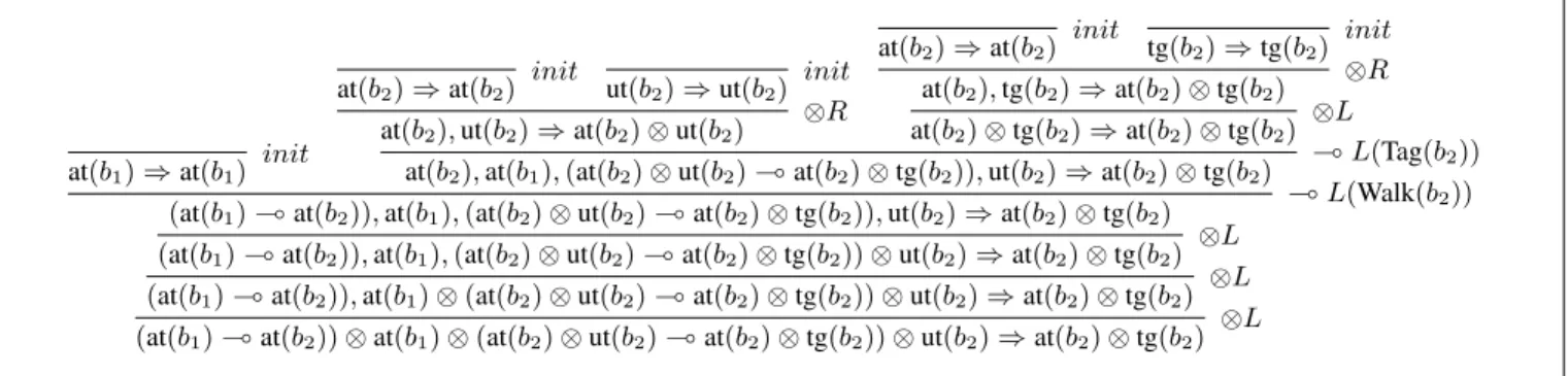
the plan. Finally, the resolved plan for this example should be the sequence of actions [Walk(b2), Tag(b2)]. The proof

tree corresponding to this example is given in Fig. 9. D. Efficient Proof Search for mini-LPL

The main idea underlying our efficient proof theory for mini-LPL is a combination of resource management ideas for linear logic [31] with formalizations of back-chaining in LHHF [13]. In particular, we define a new sequent,

∆ \ ∆O⇒ G , (2)

which indicates that the goal G can be proven using resources from the multiset ∆, leaving resources in the “output” multiset ∆O unused. Previous implementations of resource

management relied on the assumption ∆O ⊆ ∆ [31],

whereas we will allow decomposed, partial resources to be leftover for later use. The proof system we construct focuses on decomposing the goals into the smallest atomic subgoals, following which it employs back-chaining through a residuation judgment analyzing each resource in turn. This new judgment takes the form

D  γ \ ∆GB ∆O, (3)

which indicates that when the resource D is used to prove the atomic goal γ, additional subgoals in ∆G must be

proven, and the additional leftover resources in ∆O must be

considered later for consumption. Our approach eliminates the need to try different orderings of the ⊗R and ⊗L rules,

at(b1) ⇒ at(b1) init at(b2) ⇒ at(b2) init ut(b2) ⇒ ut(b2) init at(b2), ut(b2) ⇒ at(b2) ⊗ ut(b2)

⊗R at(b2) ⇒ at(b2) init tg(b2) ⇒ tg(b2) init at(b2), tg(b2) ⇒ at(b2) ⊗ tg(b2) ⊗R at(b2) ⊗ tg(b2) ⇒ at(b2) ⊗ tg(b2) ⊗L at(b2), at(b1), (at(b2) ⊗ ut(b2) ( at(b2) ⊗ tg(b2)), ut(b2) ⇒ at(b2) ⊗ tg(b2) ( L(Tag(b

2))

(at(b1) ( at(b2)), at(b1), (at(b2) ⊗ ut(b2) ( at(b2) ⊗ tg(b2)), ut(b2) ⇒ at(b2) ⊗ tg(b2) ( L(Walk(b 2))

(at(b1) ( at(b2)), at(b1), (at(b2) ⊗ ut(b2) ( at(b2) ⊗ tg(b2)) ⊗ ut(b2) ⇒ at(b2) ⊗ tg(b2)

⊗L (at(b1) ( at(b2)), at(b1) ⊗ (at(b2) ⊗ ut(b2) ( at(b2) ⊗ tg(b2)) ⊗ ut(b2) ⇒ at(b2) ⊗ tg(b2)

⊗L (at(b1) ( at(b2)) ⊗ at(b1) ⊗ (at(b2) ⊗ ut(b2) ( at(b2) ⊗ tg(b2)) ⊗ ut(b2) ⇒ at(b2) ⊗ tg(b2)

⊗L

Fig. 9. Proof tree for the goal at(b2) ⊗ tagged(b2). Predicates tagged(X) and untagged(X) have been shortened as tg(X) and ut(X), respectively.

decreasing the complexity of proof search, for which a more precise quantification will be completed in future work.

We have constructed specialized inference rules to for-mally define these sequents. In order to maintain a reasonable length, we have not included these inference rules in this paper, but interested readers can refer to [32] for details.

IV. TASKPLANNING WITH THERHEXHEXAPOD

A. Extended Domain Specification

In this section, we present extensions to the simple do-main definition we presented in Sec. III-A, incorporating support for different terrain types and associated behaviors as well as a new action for seeking specific landmarks. In particular, a path between two landmarks can now be mud, rough, smooth, allowing no movement, walking or running respectively. A new action, Seek(X) can be used by the robot to search for a specific landmark X by continually turning in place while visually scanning the environment. In addition to the definitions of Fig. 2, encodings for these additional predicates and actions are given in Fig. 10, with the walking action modified to check for the surface type.

New Predicates:

see(X) : Robot can see landmark X. surface(X, Y, Z) : Path between X and Y has type Z. New Actions:

Run(X) : Robot runs to the landmark X. Seek(X) : Robot searches for landmark X. Fig. 10. New predicates and actions in the extended planning domain.

The mini-LPL encodings of new actions introduced for the extended planning domain are given in Fig. 11. The Seek(X) action can be invoked whenever the robot can see an arbitrary landmark Y , but upon completing the action it will have found the desired landmark X. Note that this assumes the robot has a primitive behavior that is guaranteed to find the landmark being searched. The Walk(X) and Run(X) actions first check for the current location and the visibility of the target as well as the path surface, then relocate the robot to the new landmark X using the appropriate behavior. B. Experimental Setup and the Example Planning Problem

With the extended set of predicates and actions described in Sec. IV-A, we now describe a planning scenario that

Seek(X) : see(Y )( see(X)

Walk(X) : at(Y ) ⊗ see(X) ⊗ surface(Y, X, rough)( at(X) ⊗ see(X) ⊗ surface(Y, X, rough)) Run(X) : at(Y ) ⊗ see(X) ⊗ surface(Y, X, smooth)(

at(X) ⊗ see(X) ⊗ surface(Y, X, smooth) Fig. 11. Additional actions in the extended domain encoded in mini-LPL.

Fig. 12. A snapshot from the experimental setup in its initial state. Six colored landmarks are scattered throughout the environment, observable through a camera mounted on the RHex robot.

we will deploy on the physical robot. Fig. 12 shows the experimental setup with six uniquely colored landmarks. Initially, the robot is at the special location Start. Landmark tags and road surfaces between different pairs of landmarks are as given by the mini-LPL encoding of the initial state as

Di= at(Start) ⊗ untagged(b3) ⊗ untagged(b5)

⊗ surface(Start, b1, rough) ⊗ surface(b1, b0, rough)

⊗ surface(b0, b3, rough) ⊗ surface(b3, b4, smooth)

⊗ surface(b4, b2, smooth) ⊗ surface(b2, b5, smooth)

⊗ see(b0) ,

also indicating that the landmark b0 is initially visible.

In the final state, the robot is expected to be at the landmark b5and landmarks b3 and b5should be tagged. We

encode the goal state as

G = at(b5) ⊗ tagged(b3) ⊗ tagged(b5) ⊗ > .

The “truth” symbol > at the end of the goal formula is used to indicate that whichever resources are leftover at the end of the reasoning are not to be considered and can be consumed. The full LPL language incorporates this constant to increase

the expressivity of the language. Note, also, that our encoding of this planning problem does not preclude the possibility of multiple plans, which would be exposed by searching for all possible proofs for a given sequent.

C. Visual Tracking of Colored Landmarks

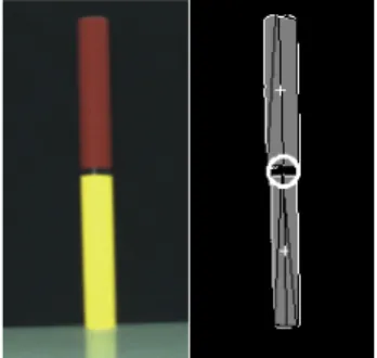
Our example domain requires navigation on the horizontal plane. Consequently, it is sufficient for RHex to find bearing and distance information associated with each landmark to be able to implement the Seek(X) action and movement between landmarks. To this end, we have chosen to use cylindrical landmarks with a height of 1.5m and a radius of 8cm each. Each landmark consists of two of three distinct colors (red, yellow and blue), whose relative ordering (top vs. bottom) distinguishes it from others. An example of such a landmark is shown on the left side of Fig. 13.

Fig. 13. Left: A red-yellow landmark as seen by the robot. Right: blobs extracted from the image with their centers marked with a “+” sign. Computed landmark location is the midpoint of the two blobs and is marked with a white circle.

The RHex robot has two on-board RTD CME137LX single-board computer units, one of which is used for visual processing of color frames captured by a Point Grey Flea2 camera at 5Hz. Our image processing algorithm first applies a color filtering algorithm based on a color model based on Mahalanobis distance in RGB space (calibrated through data collected offline) to convert the original colored image into a labeled bitmap. Connected blobs in this bitmap are then extracted using the cvBlob library [33], filtered by domain specific conditions such as blob size, aspect ratio and orientation. Subsequently, pairs of blobs are associated with each other based on their relative locations constrained by the structure of our landmark design, yielding the final landmark locations as shown in the right side of Fig. 13. Once the pair is known, landmark location is determined as the midpoint of its two blobs, and the distance to the landmark is determined through the total blob area. Robot pose information relative to the landmark is then communicated to a Matlab script running on an external computer.

D. Automatic Theorem Prover for LPL

Our implementation of the proof system described in Sec. III-D was done in SWI-Prolog. Given an initial state, action descriptions and a goal sentence in LPL, this prover will find a plan if it exists. Intuitionistic logic languages allow the annotation of proof structures with proof terms [34],

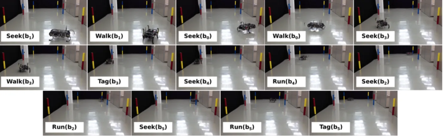
which can be used to effectively extract programs associated with these intuitionistic proofs. Our prover makes use of this idea, through which plans corresponding to the proof structure can be extracted. Implementation details of how this is performed are left outside the scope of this paper but interested readers can refer to [32]. Applied to the initial and goal states in Sec. IV-B, our LPL planner extracts the final sequence of actions as

[Seek(b1), Walk(b1), Seek(b0), Walk(b0), Seek(b3),

Walk(b3), Tag(b3), Seek(b4), Run(b4), Seek(b2),

Run(b2), Seek(b5), Run(b5), Tag(b5)] .

E. Plan Execution on RHex

As described in Sec. IV-C, visual landmark distance and bearing information is communicated back to an external workstation running a Matlab program. Our LPL theorem prover described in Sec. IV-D provides this program with a sequence of actions to be executed with the same labellings of landmarks as those identified by the visual tracker. The fi-nal plan execution system brings these components together, tracking the robot’s progress and initiating the behaviors prescribed by the plan by communicating with the control board on RHex. A sequence of snapshots for the resulting plan execution are shown in Fig. 14. The video attachment accompanying this paper shows the entire plan execution.

It is important to note that we do not address dynamic environments or unexpected disturbances in this paper. This would require explicit re-planning, for which different meth-ods have been considered in the literature [35]. Our primary contribution in this paper, however, is the formulation of the Linear Planning Logic language and an effective theorem prover for it that is capable of generating a long sequence of actions (14 total, computed in 90 seconds on a Intel Pentium Dual-Core CPU E6500 Processor 2.93GHz PC with 2 GB of RAM with an unoptimized SWI-Prolog implementation) that would have been infeasible for other methods based on theorem proving such as situational calculus.

V. CONCLUSION

In this paper, we introduced a new logical language, Linear Planing Logic (LPL), together with a robotic planner based on theorem proving methods considering both expressivity needs of planning problems as well as the efficiency of proof search. Our main contributions include the design of the language as well as a new proof theory that allows negative occurrences of linear simultaneous conjunction through care-ful resource management and elimination of nondeterminism by enabling back-chaining.

We illustrated the application of this new language and theorem prover on a hexapod robot navigating in an envi-ronment populated with colored landmarks. We presented a planning experiment where the execution of a plan ex-tracted from a formal logical proof is realized on the RHex hexapod platform. Possible future directions for this work include a more efficient implementation of the LPL theorem prover, integration with constraint expressions to interface

Fig. 14. Snapshots during the execution of the behavioral plan for RHex generated by the LPL theorem prover.

with continuous properties of robotic behaviors and reactive components to provide support for dynamic environments.

ACKNOWLEDGEMENTS

We thank to Frank Pfenning for his feedback during the formalization of Linear Planning Logic and Mehmet Mutlu for his support during our experiments. This project was partially supported by TUBITAK project 109E032.

REFERENCES

[1] P. Fiorini and E. Prassler, “Cleaning and household robots: A technol-ogy survey,” Autonomous Robots, vol. 9, pp. 227–235, Dec. 2000. [2] B. Goldstein and R. Shotwell, “Phoenix: The first Mars Scout

mis-sion,” in Proc. of the IEEE Aerospace Conf., pp. 1–20, March 2009. [3] M. Mihelj and J. Podobnik, Haptics for Virtual Reality and

Teleoper-ation, vol. 67 of Intelligent Systems, Control and Automation: Science and Engineering. Springer, 2012.

[4] T. Lozano-Perez, “Task planning,” Robot motion: planning and con-trol, pp. 463–489, 1982.

[5] S. Russel and P. Norvig, Artificial Intelligence: A Modern Approach. Prentice Hall, 1995.

[6] R. E. Fikes and N. J. Nilsson, “STRIPS: A new approach to the appli-cation of theorem proving to problem solving,” Artificial Intelligence, vol. 2, pp. 189–208, 1971.

[7] L. Chrpa, “Linear logic in planning,” in Proc. of the The Int. Conf. on Automated Planning and Scheduling, pp. 26–29, 2006.

[8] J.-Y. Girard, “Linear logic,” Theoretical Computer Science, vol. 50, no. 1, pp. 1–102, 1987.

[9] P. Kungas, “Linear logic programming for ai planning,” masters, Institute of Cybernetic at Tallinn Technical University, May 2002. [10] E. Jacopin, “Classical AI planning as theorem proving: The case of a

fragment of linear logic,” in AAAI Fall Symp. on Automated Deduction in Nonstandard Logics, (Palo Alto, CA), pp. 62–66, 1993.

[11] M. Kanovich and J. Vauzeilles, “The classical AI planning problems in the mirror of horn linear logic: semantics, expressibility, complexity,” Mathematical Structures in Computer Science, vol. 11, pp. 689–716, December 2001.

[12] C. Belta, A. Bicchi, M. Egerstedt, E. Frazzoli, E. Klavins, and G. Pappas, “Symbolic planning and control of robot motion - grand challenges of robotics,” IEEE Robotics & Automation Magazine, vol. 14, pp. 61–70, March 2007.

[13] J. S. Hodas and D. Miller, “Logic programming in a fragment of intuitionistic linear logic,” Information and Computation, vol. 110, no. 2, pp. 327–365, 1994.

[14] S. Russell and P. Norvig, Artificial Intelligence: A Modern Approach. Prentice Hall, second ed., 2003.

[15] J. S. Penberthy and D. S. Weld, “UCPOP: A sound, complete, partial order planner for adl,” in Proc. of the Int. Conf. on Knowledge Representation and Reasoning, pp. 103–114, 1992.

[16] A. L. Blum and M. L. Furst, “Fast planning through planning graph analysis,” Artificial Intelligence, vol. 90, no. 1, pp. 1636–1642, 1995.

[17] B. C. Gazen and C. A. Knoblock, “Combining the expressivity of UCPOP with the efficiency of GraphPlan,” in Proc. of the European Conf. on Planning, pp. 221–233, 1997.

[18] W. M. P. Van Der Aalst, “The application of Petri Nets to workflow management,” Journal of Circuits, Systems and Computers, vol. 08, no. 01, pp. 21–66, 1998.

[19] W. Zhang, “Representation of assembly and automatic robot planning by Petri Net,” IEEE Transactions on Systems, Man and Cybernetics, vol. 19, pp. 418–422, Mar. 1989.

[20] H. Costelha and P. U. Lima, “Robot task plan representation by Petri Nets: modelling, identification, analysis and execution,” Autonomous Robots, vol. 33, no. 4, pp. 337–360, 2012.

[21] U. Engberg, G. Winskel, and N. Munkegade, “Petri Nets as models of linear logic,” in Proceedings of Colloquium on Trees in Algebra and Programming, pp. 147–161, Springer-Verlag LNCS, 1990.

[22] M. Masseron, C. Tollu, and J. Vauzeilles, “Generating plans in linear logic I. actions as proofs.,” Theor. Comput. Sci., vol. 113, no. 2, pp. 349–370, 1993.

[23] M. Masseron, “Generating plans in linear logic: II. a geometry of conjunctive actions,” Theoretical Computer Science, vol. 113, no. 2, pp. 371–375, 1993.

[24] M. I. Kanovich and J. Vauzeilles, “Strong planning under uncer-tainty in domains with numerous but identical elements (a generic approach).,” Theoretical Computer Science, vol. 379, no. 1-2, pp. 84– 119, 2007.

[25] M. I. Kanovich and J. Vauzeilles, “Linear logic as a tool for planning under temporal uncertainty.,” Theoretical Computer Science, vol. 412, no. 20, pp. 2072–2092, 2011.

[26] L. Dixon, A. Smaill, and T. Tsang, “Plans, actions and dialogue using linear logic,” Journal of Logic, Language and Information, vol. 18, pp. 251–289, 2009.

[27] A. Rossberg, D. L. Botlan, G. Tack, T. Brunklaus, and G. Smolka, Alice Through the Looking Glass, vol. 5, pp. 79–96. Munich, Germany: Intellect Books, Feb. 2006.

[28] U. Saranli, M. Buehler, and D. E. Koditschek, “RHex: A simple and highly mobile robot,” International Journal of Robotics Research, vol. 20, pp. 616–631, July 2001.

[29] S. Thompson, Type Theory and Functional Programming. Addison-Wesley, 1991.

[30] D. Miller, G. Nadathur, F. Pfenning, and A. Scedrov, “Uniform proofs as a foundation for logic programming,” Annals of Pure and Applied Logic, vol. 51, no. 1–2, pp. 125–157, 1991.

[31] I. Cervesato, J. S. Hodas, and F. Pfenning, “Efficient resource man-agement for linear logic proof search,” Theoretical Computer Science, vol. 232, pp. 133–163, Feb. 2000.

[32] U. Saranli and S. Kortik, “Linear planning logic,” Tech. Rep. in preparation, Middle East Technical University, 2013.

[33] C. C. L. n´an, “cvBlob.” http://cvblob.googlecode.com.

[34] F. Pfenning, “Lecture notes on constructive logic,” tech. rep., Carnegie Mellon University, 2000.

[35] S. Koenig and M. Likhachev, “Fast replanning for navigation in unknown terrain,” IEEE Transactions on Robotics, vol. 21, no. 3, pp. 354–363, 2005.