Hyun Soo Nam, Chunjae Park and Oh In Kwon
IOP PUBLISHING PHYSICS IN MEDICINE AND BIOLOGY
Phys. Med. Biol. 57 (2012) 5113–5140
doi:10.1088/0031-9155/57/16/5113
Magnetic resonance electrical impedance tomography
(MREIT) based on the solution of the convection
equation using FEM with stabilization
Omer Faruk Oran and Yusuf Ziya Ider
Department of Electrical and Electronics Engineering, Bilkent University, Ankara, Turkey E-mail: [email protected]
Received 21 February 2012, in final form 30 May 2012 Published 27 July 2012
Online at stacks.iop.org/PMB/57/5113 Abstract
Most algorithms for magnetic resonance electrical impedance tomography (MREIT) concentrate on reconstructing the internal conductivity distribution of a conductive object from the Laplacian of only one component of the magnetic flux density (∇2B
z) generated by the internal current distribution. In
this study, a new algorithm is proposed to solve this ∇2B
z-based MREIT
problem which is mathematically formulated as the steady-state scalar pure convection equation. Numerical methods developed for the solution of the more general convection–diffusion equation are utilized. It is known that the solution of the pure convection equation is numerically unstable if sharp variations of the field variable (in this case conductivity) exist or if there are inconsistent boundary conditions. Various stabilization techniques, based on introducing artificial diffusion, are developed to handle such cases and in this study the streamline upwind Petrov–Galerkin (SUPG) stabilization method is incorporated into the Galerkin weighted residual finite element method (FEM) tonumericallysolvetheMREITproblem.Theproposedalgorithmistestedwith simulated and also experimental data from phantoms. Successful conductivity reconstructions are obtained by solving the related convection equation using the Galerkin weighted residual FEM when there are no sharp variations in the actual conductivity distribution. However, when there is noise in the magnetic flux density data or when there are sharp variations in conductivity, it is found that SUPG stabilization is beneficial.
(Some figures may appear in colour only in the online journal)
1. Introduction
In magnetic resonance electrical impedance tomography (MREIT), current is injected into a conductive object via surface electrodes. The resulting internal current generates a magnetic
flux density distribution both inside and outside the object. The magnetic flux density inside the object is measured using a magnetic resonance imaging (MRI) system, and from this measured magnetic flux density distribution, the internal electrical conductivity distribution of the object is reconstructed. An MRI scanner is capable of measuring only one component of the magnetic flux density, namely Bz, where z is the direction of the main static magnetic
field of the scanner. Measurement of the other components requires object rotations which are not desirable because of possible misalignments and which are in fact impossible for long objects in a conventional closed-bore MRI system. Therefore, most algorithms today concentrate on the reconstruction of the conductivity distribution from Bz only (Birgul and
Ider 1995, Ider and Birgul 1998, Seo et al 2003, Oh et al 2003, Ider and Onart 2004). Many Bz-based MREIT algorithms utilize the Laplacian of Bz, which can be expressed as
y − J
y ∂σ/∂σ x ) (Scott et al 1991), where Jx and Jy are the x- and ycomponents
(transverse components) of the injected current density distribution, σ is the electric conductivity distribution and μ is the magnetic permeability which is taken to be μ0 = 4π × 10−7 Hm−1. This expression can also be written in its modified form as
R
y − Jywhere R = lnσ (Ider and Onart 2004). If Jx and Jy are known for a
certain slice (intersection of the object with a certain z = constant plane), then the transverse gradient of R, (∂
∂Rx , ∂∂Ry ), can be calculated from the ∇2Bz data obtained for that slice only.
This is the major advantage of ∇2B
z-based algorithms because reconstruction of conductivity
at a certain slice is possible. However, the calculation of Jx and Jy for a certain slice requires
the solution of the magnetic resonance current density imaging (MRCDI) problem. It was shown by Park et al (2007) that the transverse current density distribution cannot be fully recovered using only Bz information unless the difference between the z-components of the
actual current density and the current density calculated for homogeneous conductivity is negligible. Nevertheless, Park et al (2007) have developed an algorithm by which Jx and Jy
distributions can be estimated for a certain slice given the ∇2B
z data for that slice. In their
algorithm, the ‘projected current density’ which is the recoverable portion of the actual current density is reconstructed. Nam et al (2008) used the transverse component of this ‘projected current density’ in the ∇2B
z = Ry −Jy relation to find the transverse gradient
of R for the slice of interest. Starting from the gradient distribution, Nam et al (2008) utilized
a layer potential technique,
firstsuggestedbyOhetal(2003),toreconstructtheconductivitydistributiononthat slice. Other investigators have suggested utilizing line integrals for reconstructing conductivity from its gradient (Seo et al 2003), or solving for R using the finite difference approximation (Ider and Onart 2004), or other approximations (Oran and Ider 2010) of the above relation.
In this study, it is observed that the relation ∇2B
z = Ry − Jy is in the form of the
steady-state scalar convection equation. The convection equation is a special case of the more general convection–diffusion equation. The convection–diffusion equation describes the distribution of a physical quantity (e.g. concentration and temperature) under the effect of two basicmechanisms,convectionanddiffusion.Theconvection–diffusionequationarisesinmany physical phenomena such as distribution of heat, fluid dynamics, etc. Although physically no convection mechanism exists in the MREIT problem, it can nevertheless be handled as a convection problem solely from a mathematical point of view. Furthermore, because the convection equation by itself does not always yield stable numerical solutions, introduction of a diffusion term as a stabilization technique is customary. In this study, therefore, the MREIT problem is handled as a convection–diffusion problem and the existing advanced
numerical methods for the solution of the convection–diffusion equation by using the finite element method (FEM) are used for solving the MREIT problem. The methods are then tested with simulated and experimental data.
2. Methods
2.1. Problem definition
The forward problem for Bz-based MREIT and MRCDI is given as follows: let be a connected
and bounded domain in R3 with the boundary ∂. With unit outward normal along the boundary ∂ being n, and non-zero conductivity in being σ(x,y,z) in units of S m−1, the potential field, φ(x,y,z), obeys Laplace’s equation ∇ ·σ∇φ(x,y,z) = 0 in and satisfies the Neumann condition
n g on ∂ where g is the boundary injected current density in units of A m−2 which is
non-zero only on the boundary regions where current is injected and sunk and its integral on ∂ is zero.
The electrical field E is given by E = −∇φ and it is related to the current density J by J = σE. The z-component of the magnetic flux density due to the transverse component of the current density is given by the Biot–Savart integral:
Bz(x,y,z) d . (1)
The inverse problem of Bz-based MRCDI is to find Jx and Jy from available measurements of
Bz(x,y,z) on a finite number of spatial locations in , and the inverse problem of Bz-based
MREIT is to find σ(x,y,z) from the same data.
2.2. MREIT based on the solution of the convection equation
Taking the curl of both sides of Ampere’s law (J = ∇ × H), and using the vector identity ∇ × ∇ × H = ∇(∇ · H) − ∇2H together with the facts that ∇ · H = 0 and H = B/μ
0, the following expression, which relates the x- and y-components of the current density distribution to the Laplacian of the measured magnetic flux density (Bz), is obtained:
∂Jx ∂Jy ∇2Bz
− = . (2)
∂y ∂x μ0
Since current density is given by J = σE and ∇ × E = 0, we also have
. (3) μ0
Defining R = lnσ, andJ = (−Jy,Jx), (3) can be put into the form of the scalar pure convection
equation, which is introduced and discussed in appendix A.1, as
∇2Bz
R . (4)
is the scalar field to be solved and ∇μ2B0 zis the source term. In this ‘MREIT convection
actual current density consists of two components, namely J0 and Jd, where J0 is the current density distribution obtained by solving the forward problem for the homogenous conductivity distribution and Jd is defined as the difference current density such that Jd = J − J0. Since only B
z is utilized, only an estimate for the transverse component of the difference
current density, namely J∗, can be calculated (Park et al 2007). J∗ is calculated from the relation J , where β is the solution of the two-dimensional (2D) Laplace equation given as
∇2β = ∇2Bz in and , (5)
μ0
where is the intersection of with a z = constant plane (the slice of interest) and ∂is the boundary of the intersection. Once J∗ is obtained, the transverse component of the projected substituted into (4) so that it can be solved for R. = − current density which is defined as JP
is calculated. J ( JyP,JxP) is then
For the numerical solution of (4) on the slice of interest, the FEM is used. Using FEM, (4) is transformed into a linear matrix system Sn×nRn×1 = fn×1, where n is the number of nodes
in the triangular mesh at the slice of interest, and R is the vector of unknown nodal R values. In the FEM formulation, either the standard Galerkin weighted residual method, or the Galerkin weighted residual method with streamline upwind Petrov–Galerkin (SUPG) stabilization is used. If the standard Galerkin weighted residual method is used, S and f are equal to Sg and fg which are introduced and derived in appendix A.2. If, on the other hand, the
Galerkin weighted residual method with SUPG stabilization is used, S and f are equal to Ssupg and fsupg as given in appendix A.3.
In MREIT, in general, at least two current injections are used in order to ‘guarantee’ unique conductivity reconstruction apart from a constant factor (Ider et al 2003). For the case of two current injections, if S1 and f1 denote S and f for the first current injection, and if S2 and
f2 denote S and f for the second current injection, the final matrix system to be solved is
. (6)
In solving (4), boundary conditions must also be considered. When Dirichlet boundary conditions are used, corresponding nodes on the boundary are assigned conductivity values and the matrix system in (6) is reduced accordingly. The reduced system is solved using singular value decomposition (SVD) without truncation (all singular values of the final matrix are used). The use of SVD also provides information about the singular values and hence the conditioning of the inverse problem. Some results regarding the condition numbers of various cases are given in section 4.
2.3. Simulation methods
For simulations, a cylindrical phantom of height 20 cm and diameter 9.4 cm is modelled (figure 1(a)) using Comsol Multiphysics (Comsol AB, Sweden) software package in order to
solve for electric potential in the three-dimensional (3D) forward problem explained in section
2.1. The regions into which the current is injected are 3 cm recessed from the body of the phantom to model the phantom which is used in the experiments. Current is injected through circular electrodes of diameter 1 cm located at the ends of recessed parts. Cross-section of the recessed parts is square with edges of 2.5 cm long. Current is applied between electrodes facing each other and two current injection ‘directions’, I1 (horizontal) and I2 (vertical), are used as shown in figure 1(c). Magnitude of injected current is 10 mA.
Background conductivity of the simulation phantom is taken to be 1 S m−1 and two cylindrical regions of conductivity anomaly are modelled inside the phantom. Figure 3(d) shows the conductivity distribution of the simulation phantom for the z = 0 slice. The conductivities of the low and high conductivity anomalies are 0.4 and 2.5 S m−1, respectively. However, in one case, the change of conductivity from the background value to the low and high values in the anomalous regions is not sharp but it is tapered as shown in figures 3(b) and (d). In another case, change in conductivity is sharp as shown in figure 4(b). Tetrahedral elements with quadratic shape functions are used for the FEM formulation of the 3D problem. Thereare1159225tetrahedralelementsand212007nodes(1608578degreesoffreedomsince quadraticshapefunctionsareused)intotal.Oncetheforwardproblemissolved,currentdensity distribution is obtained, by interpolation, on the nodes of a 2D triangular mesh representing
(a) (b) (c)
Figure1.(a)ThephantommodeldrawnusingComsolMultiphysics.Twocylindricalregionswhich have different conductivity from the background are also seen. The height of the first cylindrical region is 10 cm, while the height of the other cylindrical region is 8 cm. The z-direction is the direction of the main magnetic field of the MRI system. (b) Picture of the experimental phantom for the first experimental setup explained in section 2.4. The balloon inside the phantom acts as an insulator and it isolates its inside solution from the background solution. (c) Illustration of the central transverse slice of the empty phantom where z = 0. The horizontal current injection (I1)
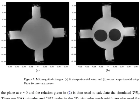
Figure 2. MR magnitude images: (a) first experimental setup and (b) second experimental setup. Units for axes are metres.
the plane at z = 0 and the relation given in (2) is then used to calculate the simulated ∇2B z.
There are 5088 triangles and 2657 nodes in the 2D triangular mesh which are also used for the solution of the convection equation (using linear shape functions).
In addition to the simulation phantom which has the same geometry as the phantom used in the experiments, other simulation phantoms which are shown in figures 6 and 7 are also utilized. Their details are explained in the respective parts of section 3.1.
The simulated ∇2B
z at the slice of interest is the input data for reconstructing the projected
transverse current density on that slice. Conductivity distribution is then reconstructed by solving (4) using the proposed method. Errors made in the transverse component of the
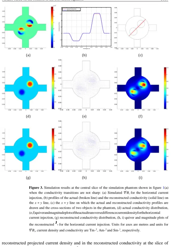
Figure 3. Simulation results at the central slice of the simulation phantom shown in figure 1(a) when the conductivity transitions are not sharp: (a) Simulated ∇2B
z for the horizontal current
injection, (b) profiles of the actual (broken line) and the reconstructed conductivity (solid line) on the x = y line, (c) the x = y line on which the actual and reconstructed conductivity profiles are drawn and the cross-sections of two objects in the phantom, (d) actual conductivity distribution, (e,f)quiverandmagnitudeplotsoftheactualtransversedifferencecurrentdensityforthehorizontal current injection, (g) reconstructed conductivity distribution, (h, i) quiver and magnitude plots of the reconstructed J∗ for the horizontal current injection. Units for axes are metres and units for ∇2B
z, current density and conductivity are Tm−2, Am−2 and Sm−1, respectively.
reconstructed projected current density and in the reconstructed conductivity at the slice of interest are calculated using the relative L2-error formulae:
) a ( −0.050 −0.04 −0.03 −0.02 −0.01 0 0.01 0.02 0.03 0.04 0.05 0.5 1 1.5 2 2.5 3 Arclength (m) Actual Conductivity Reconstructed Conductivity ) b ( (c) (d) (e) (f) (g) (h) (i)
EL2(JP) =
(7)
EL ,
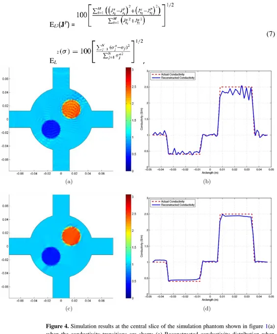
Figure 4. Simulation results at the central slice of the simulation phantom shown in figure 1(a) when the conductivity transitions are sharp: (a) Reconstructed conductivity distribution when stabilization is not used, (b) the corresponding reconstructed (solid line) and the actual (broken line) conductivity profiles on the x = y line. (c) and (d) are the same as in (a) and (b) but SUPG stabilization is utilized. Units for axes are metres and the unit for conductivity is Sm−1.
where Jxai and Jyai are the x- and y-components of the actual current density at the centre of the
ith triangle, JxPi and JyPi are the x- and y-components of the reconstructed projected current
respectively, N is the number of nodes in the 2D mesh and M is the number of the triangles in the 2D mesh.
2.4. Experimental methods
Two different experimental setups are prepared for the experiments. For the first experimental setup, a phantom, dimensions of which are the same as the simulation phantom explained in section 2.3, is manufactured. The phantom is first filled with the background solution (12 gl−1 NaCl and 1 gl−1 CuSO
4.5H2O). An insulator object is then obtained by filling a cylindricalshaped thin rubber balloon with the background solution so that the solutions inside and
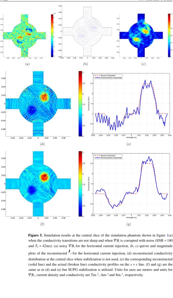
Figure 5. Simulation results at the central slice of the simulation phantom shown in figure 1(a) when the conductivity transitions are not sharp and when ∇2B
z is corrupted with noise (SNR = 180
and TC = 42ms): (a) noisy ∇2Bz for the horizontal current injection, (b, c) quiver and magnitude
plots of the reconstructed J∗ for the horizontal current injection, (d) reconstructed conductivity distribution at the central slice when stabilization is not used, (e) the corresponding reconstructed (solid line) and the actual (broken line) conductivity profiles on the x = y line. (f) and (g) are the same as in (d) and (e) but SUPG stabilization is utilized. Units for axes are metres and units for ∇2B
x 10−3 x 10⁻³
(e) (f)
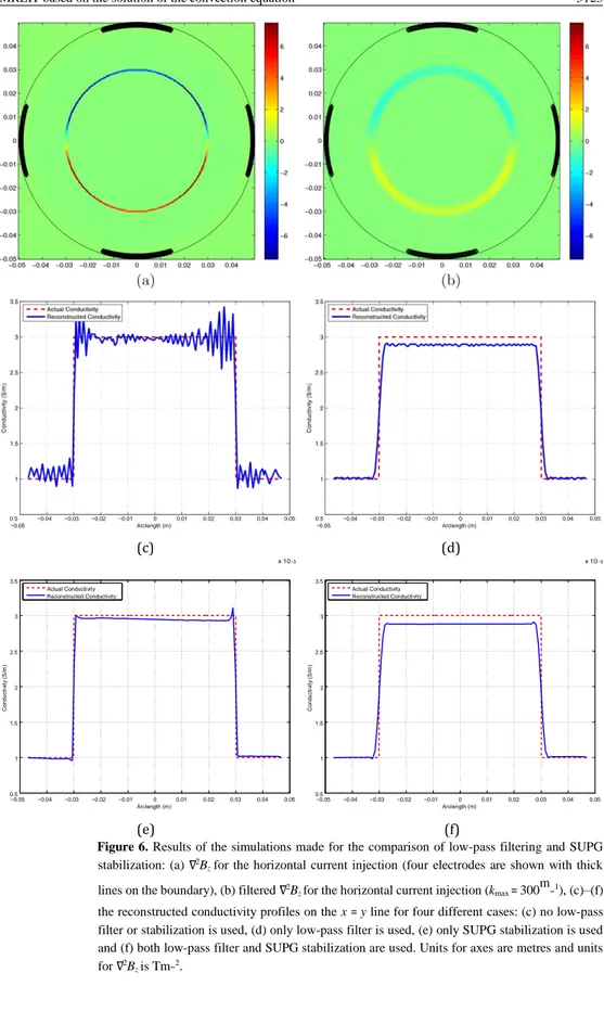
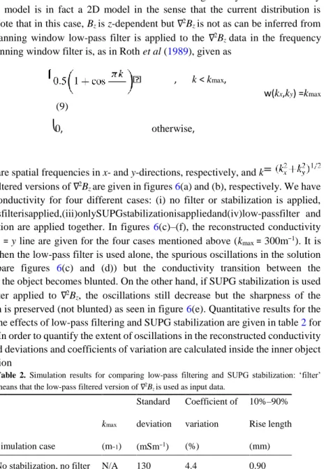
Figure 6. Results of the simulations made for the comparison of low-pass filtering and SUPG stabilization: (a) ∇2B
z for the horizontal current injection (four electrodes are shown with thick
lines on the boundary), (b) filtered ∇2B
z for the horizontal current injection (kmax = 300
m
−1), (c)–(f) the reconstructed conductivity profiles on the x = y line for four different cases: (c) no low-pass filter or stabilization is used, (d) only low-pass filter is used, (e) only SUPG stabilization is used and (f) both low-pass filter and SUPG stabilization are used. Units for axes are metres and units for ∇2B z is Tm−2. 0.5 −0.05 −0.04 −0.03 −0.02 −0.01 0 0.01 Arclength (m) (c) 0.02 0.03 0.04 0.05 0.5 −0.05 −0.04 −0.03 −0.02 −0.01 0 0.01 Arclength (m) (d) 0.02 0.03 0.04 0.05 −0.05 −0.04 −0.03 −0.02 −0.01 0 0.01 0.02 0.03 0.04 0.05 0.5 1 1.5 2 2.5 3 3.5 Arclength (m) Actual Conductivity Reconstructed Conductivity −0.05 −0.04 −0.03 −0.02 −0.01 0 0.01 0.02 0.03 0.04 0.05 0.5 1 1.5 2 2.5 3 3.5 Arclength (m) Actual Conductivity Reconstructed Conductivity
(a) (b) (c)
(d) (e) (f)
(g) (h)
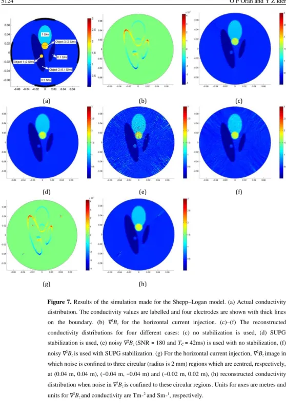
Figure 7. Results of the simulation made for the Shepp–Logan model. (a) Actual conductivity distribution. The conductivity values are labelled and four electrodes are shown with thick lines on the boundary. (b) ∇2B
z for the horizontal current injection. (c)–(f) The reconstructed
conductivity distributions for four different cases: (c) no stabilization is used, (d) SUPG stabilization is used, (e) noisy ∇2B
z (SNR = 180 and TC = 42ms) is used with no stabilization, (f)
noisy ∇2B
z is used with SUPG stabilization. (g) For the horizontal current injection, ∇2Bz image in
which noise is confined to three circular (radius is 2 mm) regions which are centred, respectively, at (0.04 m, 0.04 m), (−0.04 m, −0.04 m) and (−0.02 m, 0.02 m), (h) reconstructed conductivity distribution when noise in ∇2B
z is confined to these circular regions. Units for axes are metres and
units for ∇2B
z and conductivity are Tm−2 and Sm−1, respectively.
outside the balloon have no contact (figure 1(b)). Current is injected through electrodes facing each other and data are obtained for two current injections. The MR magnitude image for this experimental setup is given in figure 2(a). Since the balloon is filled with the background
solution, the region inside the balloon is indistinguishable from the background, with the thin boundary of the balloon being slightly perceptible. Bz is measured at three consecutive (no
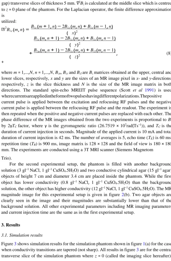
gap) transverse slices of thickness 5 mm. ∇2B
z is calculated at the middle slice which is centred
to z = 0 plane of the phantom. For the Laplacian operator, the finite difference approximation is
+
where m = 1,...,N, n = 1,...,N, Bzu, Bzc and Bzl are Bz matrices obtained at the upper, central and
lower slices, respectively, x and y are the sizes of an MR image pixel in x- and y-directions, respectively, z is the slice thickness and N is the size of the MR image matrix in both directions. The standard spin-echo MREIT pulse sequence (Scott et al 1991) is used wherecurrentsareappliedintheformoftwopulseshavingdifferentpolarizations.Thepositive current pulse is applied between the excitation and refocusing RF pulses and the negative current pulse is applied between the refocusing RF pulse and the readout. The experiment is then repeated when the positive and negative current pulses are replaced with each other. The phase difference of the MR images obtained from the two experiments is proportional to Bz
by 2γTC factor, where γ is the gyromagnetic ratio (26.7519 × 10⁷rad(Ts−1)), and TC is the
duration of current injection in seconds. Magnitude of the applied current is 10 mA and total duration of current injection is 42 ms. The number of averages is 5, echo time (TE) is 60 ms,
repetition time (TR) is 900 ms, image matrix is 128 × 128 and the field of view is 180 × 180
mm. The experiments are conducted using a 3T MRI scanner (Siemens Magnetom Trio).
For the second experimental setup, the phantom is filled with another background solution (3 gl−1 NaCl, 1 gl−1 CuSO4.5H2O) and two conductive cylindrical agar (15 gl−1 agar) objects of height 7 cm and diameter 3.4 cm are placed inside the phantom. While the first object has lower conductivity (0.8 gl−1 NaCl, 1 gl−1 CuSO
4.5H2O) than the background solution, the other object has higher conductivity (12 gl−1 NaCl, 1 gl−1 CuSO4.5H2O). The MR magnitude image for this experimental setup is given in figure 2(b). Two agar objects are clearly seen in the image and their magnitudes are substantially lower than that of the background solution. All other experimental parameters including MR imaging parameters and current injection time are the same as in the first experimental setup.
3. Results
3.1. Simulation results
Figure 3 shows simulation results for the simulation phantom shown in figure 1(a) for the case when conductivity transitions are tapered (not sharp). All results in figure 3 are for the central transverse slice of the simulation phantom where z = 0 (called the imaging slice hereafter). utilized: 2 B zc m n B zc m 1 n 2 B zc m n B zc m 1 n x 2 B zc m n 1 2 B zc m n B zc m n 1 y 2 B zu m n 1 2 B zc m n B zl m n 1 z 2 (8)
takes non-zero values only in the regions where conductivity changes, as expected from (3). Quiver plots of the actual transverse difference current density and of the reconstructed J∗ are shown in figures 3(e) and (h). In addition, their magnitude plots are given in figures 3(f) and (i). The L2 error made in the reconstructed J∗ relative to the actual transverse difference current density is 20.9%. However in the MREIT convection equation, in practice, the transverse component of the projected current density, JP, is used, and the L2 error made in JP relative to
the actual transverse current density is 0.53%. Considering (2) and (5), ∇2B
z may be thought
of as a vortex source and the actual transverse difference current density and J∗ rotate around the regions where ∇2B
z takes non-zero values as shown in figures 3(e) and (h).
The actual conductivity distribution and the conductivity distribution reconstructed using the Galerkin weighted residual FEM without stabilization are shown in figures 3(d) and (g), respectively. In addition, the reconstructed and the actual conductivity profiles on the x = y line are shown in figure 3(b). Two current injections (I1 and I2 directions in figure 1(c)) are utilized. Conductivity values on the boundary are assumed to be 1 S m−1 (R = 0 since R = lnσ). The relative L2 error made in the reconstructed conductivity is 0.84%. When SUPG stabilization is used, no significant improvement, regarding the relative L2 error, is obtained in the reconstructed conductivity distribution. Note that, in the simulation phantom investigated, since the conductivity transition regions between the background and the objects are tapered, the solution (conductivity) does not have sharpvariations and therefore successful conductivity reconstruction is possible without stabilization. Throughout this paper, by ‘sharp variations in the solution’, we mean local regions in which the solution has a steep gradient.
The algorithm is also tested when the conductivity distribution at the imaging slice has sharp variations. For this purpose, the phantom geometry same as in the previous case is used with narrower conductivity transition regions. The actual conductivity profile on the x = y line at the imaging slice is given in figures 4(b) and (d) by the broken lines. Figures 4(a) and (b) show the conductivity reconstructions when no stabilization is utilized. The relative L2 error made in the reconstructed conductivity is 5.71% and considerable oscillations are observed. However, when SUPG stabilization is used, the relative L2 error decreases to 2.84% and oscillations disappear as shown in figures 4(c) and (d). Therefore, although stabilization is not found to be necessary when conductivity variations are not sharp, it is found that for objects in which conductivity variations are sharp and abrupt, stabilization becomes necessary. Performance of the algorithm against noise in measurement data is also investigated. The noise in Bz is assumed to have a zero-mean Gaussian distribution with standard deviation σBz
= 1/(2γTCSNR), where γ is the gyromagnetic ratio, TC is the duration of current injection in
seconds and SNR is the signal-to-noise ratio of the MR complex image (Scott et al 1992). In the simulations, SNR values of 60, 90, 120 and 180 are used. This range of values includes the SNR values estimated from the MR magnitude images obtained in the experiments. For estimation, we have selected a smooth region in the MR magnitude image and calculated the√ average of the magnitude in this region. The average is then divided by s 2, where s is the standard deviation of the magnitude image which is again obtained in the same region. As√
discussed by Sadleir et al (2005), the 2 factor is due to the fact that s is calculated from the magnitude image rather than the complex image. For the experimental phantoms used in this study, SNR is estimated to be in the range 70–100. Note that, since SNR is also
a function of pixel size, in the simulations we have used the same pixel sizes as in the experiments.
In practice, one needs to know Bz in three consecutive slices in the z-direction in order to
calculate∇2B
z usingthefinitedifferenceapproximationgivenin(8).However,forsimulations, we
use the relation given in (2) to calculate ∇2B
z. In this case, in order to calculate the noise image
which will be added to ∇2B
z, the following steps are followed: let Gu, Gc and Gl be the
Gaussian-distributed noise images representing the noise in Bz at upper, central and lower
slices, respectively, each of which is calculated independently for the same specific SNR and TC. ∇2G is calculated using (8) by replacing Bz with G and it is then added to ∇2Bz which is
calculated using (2). Using this procedure for obtaining noisy ∇2B
z, we have made simulations
for the phantom shown in figure 1(a) when the conductivity transitions are not sharp as shown in figures 3(b) and (d). Noisy ∇2B
z, the quiver and the magnitude plots of J∗ obtained using
the noisy ∇2B
z are given in figures 5(a)–(c), respectively, when SNR = 180 and TC = 42ms. The
reconstructed conductivity distribution and conductivity profile on the x = y line are given at the imaging slice in figures 5(d) and (e) when no stabilization is applied and in figures 5(f) and (g) when SUPG stabilization is applied. Two current injections are utilized in
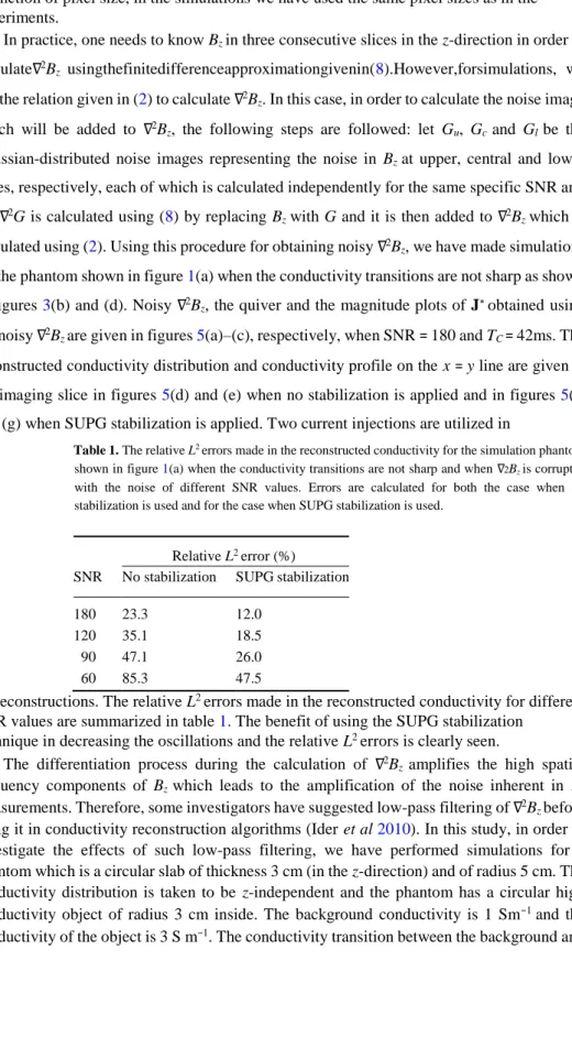
Table 1. The relative L2 errors made in the reconstructed conductivity for the simulation phantom
shown in figure 1(a) when the conductivity transitions are not sharp and when ∇2Bz is corrupted
with the noise of different SNR values. Errors are calculated for both the case when no stabilization is used and for the case when SUPG stabilization is used.
Relative L2 error (%)
SNR No stabilization SUPG stabilization
180 23.3 12.0
120 35.1 18.5
90 47.1 26.0
60 85.3 47.5
all reconstructions. The relative L2 errors made in the reconstructed conductivity for different SNR values are summarized in table 1. The benefit of using the SUPG stabilization
technique in decreasing the oscillations and the relative L2 errors is clearly seen. The differentiation process during the calculation of ∇2B
z amplifies the high spatial
frequency components of Bz which leads to the amplification of the noise inherent in Bz
measurements. Therefore, some investigators have suggested low-pass filtering of ∇2B z before
using it in conductivity reconstruction algorithms (Ider et al 2010). In this study, in order to investigate the effects of such low-pass filtering, we have performed simulations for a phantom which is a circular slab of thickness 3 cm (in the z-direction) and of radius 5 cm. The conductivity distribution is taken to be z-independent and the phantom has a circular high conductivity object of radius 3 cm inside. The background conductivity is 1 Sm−1 and the conductivity of the object is 3 S m−1. The conductivity transition between the background and
z-direction) electrodes facing each other. Magnitude of the injected current is 10 mA and two current injection directions are used. With this electrode geometry and conductivity distribution, the model is in fact a 2D model in the sense that the current distribution is zindependent. Note that in this case, Bz is z-dependent but ∇2Bz is not as can be inferred from
(2) or (3). A Hanning window low-pass filter is applied to the ∇2B
z data in the frequency
domain. The Hanning window filter is, as in Roth et al (1989), given as , k < kmax,
w(kx,ky) =kmax
(9)
⎩0, otherwise,
where kx and ky are spatial frequencies in x- and y-directions, respectively, and k
. Original and filtered versions of ∇2B
z are given in figures 6(a) and (b), respectively. We have
reconstructed conductivity for four different cases: (i) no filter or stabilization is applied, (ii)onlylow-passfilterisapplied,(iii)onlySUPGstabilizationisappliedand(iv)low-passfilter and SUPG stabilization are applied together. In figures 6(c)–(f), the reconstructed conductivity profiles in the x = y line are given for the four cases mentioned above (kmax = 300m−1). It is observed that when the low-pass filter is used alone, the spurious oscillations in the solution decrease (compare figures 6(c) and (d)) but the conductivity transition between the background and the object becomes blunted. On the other hand, if SUPG stabilization is used without any filter applied to ∇2B
z, the oscillations still decrease but the sharpness of the
transition region is preserved (not blunted) as seen in figure 6(e). Quantitative results for the comparison of the effects of low-pass filtering and SUPG stabilization are given in table 2 for different cases. In order to quantify the extent of oscillations in the reconstructed conductivity images, standard deviations and coefficients of variation are calculated inside the inner object in a circular region
Table 2. Simulation results for comparing low-pass filtering and SUPG stabilization: ‘filter’ means that the low-pass filtered version of ∇2B
z is used as input data.
Standard Coefficient of 10%–90%
kmax deviation variation Rise length
Simulation case (m−1) (mSm−1) (%) (mm)
No stabilization, no filter N/A 130 4.4 0.90
No stabilization, filter 600 31 1.1 2.1
No stabilization, filter 500 21 0.75 2.3
No stabilization, filter 400 17 0.60 2.5
No stabilization, filter 300 13 0.45 3.3
SUPG, no filter N/A 12 0.41 0.97
SUPG, filter 600 2.0 0.070 2.1
SUPG, filter 500 1.5 0.051 2.3
SUPG, filter 300 1.8 0.062 3.3
of radius 2.3 cm (coefficient of variation is defined as the standard deviation over mean). In order to quantify the blunting effect of low-pass filtering on the transition region, the ‘rise length’ of the transition is calculated. Rise length is defined as the distance between the points corresponding to 10% and 90% of the conductivity increase in the transition region.
As seen in table 2, without any stabilization and low-pass filter, the coefficient of variation of the oscillations inside the inner object is 4.4% and the rise length of the transition region is 0.90 mm. With the use of the low-pass filter, as the filter cut-off frequency (kmax) is lowered from 600 to 300m−1, the coefficient of variation decreases to as low as 0.45% and the rise length increases to as high as 3.3 mm. These results mean that as kmax is lowered, oscillations decrease but the spatial resolution gets poorer. On the other hand, using SUPG stabilization alone without any low-pass filter, one still obtains a low coefficient of variation of the oscillations (0.41%) but the sharpness of the transition region is preserved (rise length is 0.97 mm). When the low-pass filter and SUPG stabilization are applied together, the coefficient of variation of the oscillations decreases foralmost another order of magnitude compared to the case when only SUPG stabilization is used, although spatial resolution is again compromised.
We have so far assumed relatively simple geometries for the simulation objects. Next, a more detailed model which resembles the standard Shepp–Logan model is used (Shepp and Logan 1974, Park et al 2004). A circular slab of radius 7.5 cm and thickness (in the zdirection)of3cmisassumed.Theconductivityofthemodelistakentobez-independentandits distributioninthexy-planeisgiveninfigure7(a)wheretheconductivityvaluesarelabelled.All conductivity transitions are discontinuous. Magnitude of the injected current is 10 mA. Current isinjectedthrough3cm(arclength)longand3cmhigh(inthez-direction)opposingelectrodes on the boundary and two current injections are used. ∇2B
z for the
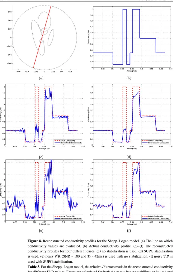
horizontal current injection is given in figure 7(b). The reconstructed conductivity distribution is shown in figure 7(c) when no stabilization is used. It is observed that the reconstruction is very successful, all regions of different conductivity are distinguishable and the sharpness of the conductivity transition regions is preserved. Some oscillating (wiggling) behaviour is observed, and this behaviour is completely lost when SUPG stabilization is used as shown in figure 7(d). This is also evident from figures 8(c) and (d) where the reconstructed conductivity profile on the line of figure 8(a) is shown without and with stabilization, respectively. The relative L2 error made in the reconstructed conductivity is 18.3% and 18.0% without and with SUPG stabilization, respectively.
(c) (d)
(e) (f)
Figure 8. Reconstructed conductivity profiles for the Shepp–Logan model. (a) The line on which conductivity values are evaluated. (b) Actual conductivity profile. (c)–(f) The reconstructed conductivity profiles for four different cases: (c) no stabilization is used, (d) SUPG stabilization is used, (e) noisy ∇2B
z (SNR = 180 and TC = 42ms) is used with no stabilization, (f) noisy ∇2Bz is
used with SUPG stabilization.
Table 3. For the Shepp–Logan model, the relative L2 errors made in the reconstructed conductivity
for different SNR values. Errors are calculated for both the case when no stabilization is used and for the case when SUPG stabilization is used.
Relative L2 error (%)
SNR No stabilization SUPG stabilization
180 31.1 19.4
120 41.9 21.2
90 54.7 23.8
60 88.9 31.9
In the simulations made for the Shepp–Logan model, average conductivity values of the constant conductivity anomalies are found to be within 5% of the actual values except for the regions where the local conductivity contrast is high such as objects 1 and 3. For instance, for object 1, the reconstructed conductivity is around 0.5 S m−1 rather than the actual value of 2 S m−1 (see figure 8(c)). Possible reasons for this error are discussed in section 4.
We have also made conductivity reconstructions for the Shepp–Logan model when the input data (∇2B
z) are noisy. The noise image which is added to ∇2Bz is calculated using the
procedure discussed above (TC = 42ms). Note that in this Shepp–Logan model, the magnitude
of the current density and so Bz at any slice is inversely proportional to the height of the
circular slab. We have set the height of the model to 3 cm so that Bz at the central slice is in
the same order of magnitude as Bz measured in the experiments for the 3D phantom shown in
figure 1(b). By this adjustment, we have been able to use the same SNR values that are used for calculating the noise for the 3D phantom. When SNR = 180, the reconstructed conductivity distributions are given in figures 7(e) and (f) when no stabilization is used and when SUPG stabilization is used, respectively. The conductivity profiles of these figures are given in figures 8(e) and (f), respectively. The conductivity reconstruction is again successful, and the sharpness of the conductivity transitions is preserved. The relative L2 errors made in the reconstructed conductivity for different SNR values are given in table 3.
For the Shepp–Logan model, another simulation is made in which the noise added to ∇2B z
is confined to distinct small regions. This noisy ∇2B
z is given in figure 7(g) for the horizontal
current injection and is obtained again using the procedure discussed above (TC = 42ms). This
time the noise image (∇2G) is masked to take non-zero values in only three distinct small regions (SNR = 60). The reconstructed conductivity for this case is given in figure 7(h). SUPG stabilization is used during the reconstruction process. It is observed that the errors in the reconstructed conductivity are also confined to the regions where the noise in ∇2B
z exists, and
the relative L2 error made in the reconstructed conductivity is 18.1%.
3.2. Experimental results
Results for the first experimental setup explained in section 2.4 are given in figures 9 and 10. Figures 9(a) and (d) show Bz measured at the central slice of the phantom (called the imaging
slice hereafter) for two current injections. Figures 9(b) and (e) show the ‘masked’ ∇2B z which
and also has high magnitude in these regions. Also Bz measurements near the boundary of the
phantom have relatively high noise probably due to the partial volume effect in MR voxels here. Therefore, ∇2B
z data are masked such that only ∇2Bz calculated in the circular region
Figure9.Inputdataandthereconstructedcurrentdensitiesforthefirstexperimentalsetupexplained in section 2.4. (a) Measured Bz for the horizontal current injection, (b) ∇2Bz calculated from Bz
measured for the horizontal current injection, (c) filtered version of ∇2B
z for the horizontal current
injection (kmax = 400m−1). (d)–(f) are the same as in (a)–(c) but obtained for the vertical current
injection. (g) and (h) The quiver and magnitude plots of J∗ reconstructed from ∇2B
z in (c). Units
of radius 0.045 m is used and outside of this region, including recessed parts, ∇2B
z is taken as
zero (in fact in theory ∇2B
z = 0 in these regions since the conductivity is constant). All
conductivity reconstructions for the experiments are made using two current injections. Several cases are considered for the conductivity reconstruction using experimental data and for some cases the Hanning window low-pass filter, which is discussed in section 3.1, is applied to the ∇2B
z data before reconstruction. Figures 9(c) and (f) show the low-pass filtered
versions of the ∇2B
z data for two current injections. The cut-off frequency (kmax) should be chosen separately for each experimental setup. One of the factors which should be considered is the SNR of the MR image and the other is the fact that the choice of kmax sets a lower bound
Figure 10. Reconstructed conductivity distributions at the central slice of the phantom for the first experimental setup explained in section 2.4. (a) Reconstructed conductivity distribution, (b) reconstructed conductivity profile on the x = y line. (a) and (b) are obtained when the original ∇2B
z
(no filter) is used without stabilization. (c) and (d) are the same as in (a) and (b) but the filtered ∇2B
z (kmax = 400m−1) is used without stabilization. (e) and (f) are the same as in (a) and (b) but the
original ∇2B
z (no filter) is used with SUPG stabilization. (g) and (h) are the same as in (a) and (b)
but the filtered ∇2B
for the spatial resolution of the reconstructed conductivity. For the experimental data given in figure 9, kmax is chosen as 500 or 400 m−1 depending on whether SUPG stabilization is used or not (the effect of SUPG stabilization on the choice of kmax is discussed in the next paragraph). The quiver and magnitude plots of J∗ reconstructed from the filtered ∇2B
z (kmax = 400m−1) are shown in figures 9(g) and (h).
Infigures10(a)and(b),thereconstructedconductivitydistributionandconductivityprofile on the x = y line are given at the imaging slice when the ∇2B
z data shown in figures 9(b) and (e)
are used without any stabilization. The reconstructed conductivity suffers from spurious oscillations. When the low-pass filtered versions of ∇2B
z data (figures 9(c) and (f)) are used
(kmax = 400m−1), the oscillations in the reconstructed conductivity decrease as shown in figures
10(c) and (d). On the other hand, when the original ∇2B
z data (no filter) are used with SUPG
stabilization, similar to the case when ∇2B
z is low-pass filtered, the oscillations in the
reconstructed conductivity are decreased as shown in figures 10(e) and (f). For the last case, figures 10(g) and (h) show the reconstructed conductivity when the filtered versions of ∇2B
z
and SUPG stabilization are used together. In this case, kmax is chosen to be 500m−1 which is higher than the case when only low-pass filtering is used. Since low-pass filtering and SUPG stabilization are utilized together, it is possible to obtain a stable solution with a higher kmax (better spatial resolution). Therefore, SUPG stabilization is still beneficial in the cases when ∇2B
z is low-pass filtered.
Results for the second experimental setup explained in section 2.4 are given in figure 11. Figures 11(a) and (b) show Bz measured at the imaging slice for two current injections. Since
MR signals coming from the agar objects are relatively low (see figure 2(b)), the measured Bz
data in these regions are greatly corrupted with noise. Therefore, all reconstructions are done with low-pass filtered versions of ∇2B
z data. The Hanning window filter explained in section 3.1 is used with kmax = 300m−1. Figures 11(c) and (d) show the low-pass filtered ∇2Bz data for
two current injections. Figure 11(e) shows the reconstructed conductivity distribution atthecentralsliceofthephantomwhennostabilizationisused.Thisreconstructedconductivity distribution suffers from oscillations. Figure 11(f) shows the reconstructed conductivity distribution when SUPG stabilization is used. The oscillations in the solution decrease and the conductivity is well reconstructed.
4. Discussion
In this study, a new MREIT algorithm is proposed to reconstruct conductivity distribution at a slice of interest given the ∇2B
z data for that slice. The relation between conductivity and ∇2Bz
data is formulated as a steady-state scalar convection equation as given in (4) and reconstruction of conductivity is achieved by the numerical solution of the convection equation using FEM. Effects of including stabilization in the FEM formulation are also investigated. Reconstructed conductivity distributions using both simulated and experimental
the MREIT problem is handled as the solution of a scalar convection equation.
It is well known that the numerical solution of the pure convection equation using the Galerkin weighted residual FEM is unstable and gives inaccurate results if the actual solution includes sharp variations (Knobloch 2009). Sharp variations in the solution may be due to internal narrow regions where the solution has a steep gradient or due to inconsistent Dirichlet boundary conditions. If the R values which are specified as the Dirichlet boundary condition on the outlet boundary, on whichJ n > 0, are inconsistent, then the solution will have sharp on the inlet boundary, on which J · n < 0 (n being the outward normal to the boundary), and variations near the outlet boundary (please see appendix· A.1 for a one-dimensional example).
Figure 11. Input data and the reconstructed conductivity distributions for the second experimental setupexplainedinsection2.4:(a,b)MeasuredBz distributionsforthehorizontalandverticalcurrent
injections,respectively,(c,d)filtered∇2B
z (kmax = 300m−1)forthehorizontalandverticalcurrent
metres and units for Bz, ∇Bz and conductivity are T, Tm− and Sm−, respectively.
The instability of the numerical solution, which is caused by any sharp variation in the solution, may be overcome by choosing a stabilization technique which in effect adds a diffusion term to the partial differential equation. In this study, the SUPG stabilization technique is used.
It is shown in figures 3(g) and (b) that when the actual conductivity distribution does not have sharp variations, the Galerkin weighted residual FEM formulation without stabilization gives accurate reconstruction results. However, for the case when the conductivity distribution has sharp variations, spurious oscillations occur in the solution and an accurate solution is not obtained as shown in figures 4(a) and (b). These oscillations disappear with the use of SUPG stabilization as shown in figures 4(c) and (d) and the relative L2 error made in the reconstructed conductivity is lower. Therefore, if the actual conductivity distribution has sharp variations, stabilization improves the accuracy of the solution by means of reducing the oscillations in the solution.
In practice, noise is inherent in the measurement of Bz and robustness of the proposed
algorithm against noise must also be investigated. Noise in Bz simulations is modelled by using
the noise model given in Scott et al (1992). Two current injections are used for all reconstructions using noisy data. Considering (4), there is a linear relation between ∇2B
z and
∇R assuming thatJ is previously calculated. Therefore, existence of any sharp variation in the∇ ∇ solution (existence of high slope narrow or local regions) implies localized high magnitude and narrow extrema in 2B
z. Considering the reverse, if 2Bz is corrupted with noise such that it
has localized high magnitude and narrow extrema, then there will be sharp variations in the solution. We think that the sharp variations in the solution due to the noise in ∇2B
z cause
spurious oscillations as shown in figures 5(d) and (e). When stabilization is used, these oscillations are reduced as seen in figures 5(f) and (g) and the relative L2 error made in reconstructed conductivity is lower (see table 1). Therefore, stabilization is useful in reducing oscillations due to sharp variations in the solution caused by noise in ∇2B
z.
We have also shown that low-pass filtering of ∇2B
z by itself helps decrease oscillations in
the solution. To discuss the effect of this low-pass filtering on decreasing oscillations, let us first consider simulated noise-free ∇2B
z distributions given in figures 6(a) and 7(b): the
corresponding conductivity distributions for these ∇2B
z distributions have jumps in transitions
between the objects and the background. For such conductivity variation, ∇2B
z is most
pronounced at object boundaries. Actually, this behaviour is evident from (3) such that ∇2B z
takes non-zero values only in regions where conductivity changes. In theory, a step change in conductivity at an internal boundary means a ∇2B
z of line impulse type. If such a ∇2Bz
distribution is low-pass filtered, then the impulsive behaviour is lost such that ∇2B z at the
low-pass filtered version of ∇2B
z distribution in figure 6(a) is given. The end effect of
conductivity reconstruction from such a low-pass filtered ∇2B
z is that step changes in
conductivity are tapered. Since sharp variations in conductivity are lost, spurious oscillations in the solution decrease. On the other hand, as discussed in the previous paragraph, if ∇2B
z is
noisy, it has localized high magnitude and narrow extrema which cause sharp variations in the solution. In such a case, when ∇2B
z is low-pass filtered, these extrema are widened and the
magnitudes of the extrema are lowered and thus sharp variations in the solution are also tapered. Therefore, the spurious oscillations due to sharp variations in the solution are also decreased.
We have discussed above that both SUPG stabilization and low-pass filtering of ∇2B z are
beneficial for decreasing the oscillations in the solution due to sharp variations. These sharp variations may be caused by either sharp conductivity transition regions or the noise in ∇2B
z.
Therefore, low-pass filtering of ∇2B
z and stabilization techniques may at first be considered as
alternatives to each other. For comparison of the two techniques, we have performed a simulation for a 2D circular phantom (figure 6) which has a discontinuous conductivity transition between the inner object and the background. Observing the standard deviations or coefficients of variation given in table 2, a beneficial effect of decreasing oscillations in the solution is observed for both low-pass filtering and SUPG stabilization. However, low-pass filtering results in poorer spatial resolution as supported by the rise length values given in table 2. Therefore, SUPG stabilization is preferred to low-pass filtering in order to preserve sharp conductivity transitions and thus to obtain better spatial resolution. However, in cases when low-pass filtering is found to be necessary due to excessive noise, use of SUPG together with low-pass filtering may become beneficial by allowing for a higher cut-off frequency for the low-pass filter. We have in fact observed this benefit when conductivity distributions are reconstructed using experimental data as shown in figure 10.
In a general sense, the solution of (4) may be thought of as taking the line integral of ∇R along the direction of the convective field. For the solution of a similar equation, Seo et al (2003) have suggested using line integrals in order to reconstruct σ from its known gradient. In this case, it is obvious that if noisy ∇2B
z is used, the error in σ tends to accumulate along the
line (Oh et al 2003). In this study, we use FEM for the solution of (4). No line integrals are calculated but the solution is obtained by solving a matrix equation. This matrix equation is solved for the whole domain. For instance, consider the reconstructed conductivity distribution given in figure 7(h). This conductivity is obtained from the ∇2B
z distribution given
in figure 7(g) which takes high values in some small distinct regions simulating the presence of localized high magnitude noise. We see that the error in conductivity is also confined to small regions where ∇2B
proposed algorithm.
In the simulations made with the Shepp–Logan model, it is observed that the proposed algorithm successfully reconstructs the conductivity distribution profile. However, in some regions where the local conductivity contrast is high, e.g. around objects 1 and 3 (see figures
7 and 8), the absolute value of the reconstructed conductivity does not agree with the actual conductivity value. Note that, the conductivity of object 1 is 2 S m−1 and it is surrounded by object 2 which has conductivity of 0.1 S m−1. Therefore, the relative local contrast of the conductivity of object 1 is high. We have carried out additional simulations to see how reconstructed conductivity depends on the relative local contrast. If the actual conductivity of object 1 is between 0.1 and 0.2 S m−1, it is reconstructed with less than 5% error. However as the contrast increases, the reconstructed value depicts a saturating behaviour and no matter how large the actual conductivity is, the reconstructed conductivity stays around 0.5 S m−1. We have also observed that the current distribution in and around object 1 does not change much if the relative contrast of object 1 is increased beyond 5. Similarly, ∇2B
z around the
boundary of object 1 also saturates. Therefore, we conclude that the conductivity of a small high contrast anomaly cannot be reconstructed exactly due to the saturating behaviour of the current distribution and ∇2B
z. This behaviour is a peculiarity of MREIT in general, and not of
the convection-equation-based reconstruction proposed in this paper.
We have used SVD to analyse the conditioning of the system matrices S1 and S2 expressed
in (6). For example for the case of the simulations shown in figure 3, the following condition numbers are obtained. When no stabilization is used, the reduced S1 and S2 matrices (after
imposing the Dirichlet boundary conditions) have condition numbers (ratio of largest singular value to the smallest one) of 1.9 × 10⁶ and 1.2 × 10⁶, respectively. However, the combined system matrix [S1;S2] representing the two current injection case has a condition number of
1187.Wehavealsoobservedthattheuseofstabilizationfurtherdecreasestheconditionnumber to 759. These results and the condition numbers that we have observed for other simulations show that the two current injection case is significantly well conditioned compared to the single current injection cases. Stabilization may somewhat improve the condition number but this is not an order of magnitude improvement.
In all reconstructions made using both simulated and experimental data, the conductivity values at the boundary are assumed to be known. In experiments conducted by phantoms, this informationisavailablesincetheconductivityofbackgroundsolutionisknown.Furthermorein experiments that would be conducted using human or animal subjects, this information is available when large carbon hydro-gel electrodes are used or the subject is covered with conductive gel pads with appropriate conductivity (Kim et al 2009).
Seo et al (2003) have also proposed a ∇2B
z-based algorithm for the reconstruction of
conductivity and later it was modified and named as the Harmonic Bz
algorithm (Oh et al 2003). This is an iterative algorithm and at each iteration the equation ∇2 , where
first iteration,= − E is calculated for a uniform conductivity distribution and for other iterations it2 E ( Ey,Ex) and Ex, Ey are the x- and y-components of the electric field, is used. At the
is calculated using the conductivity from the previous iteration. This equation is in the same convection equation form as the equation ∇ that we used in this study. Therefore, the solution methods that we have suggested can also be applied to reconstruct the conductivity at each iteration of the Harmonic Bz algorithm.
We had previously proposed an algorithm (Ider and Onart 2004) based on the finite difference discretization of . However, the method proposed in this study uses FEM and the triangular mesh of the solution domain provides a more handy method for real objects with an irregular boundary.
There are many FEM software packages which use advanced numerical techniques for the solution of partial differential equations. Comsol Multiphysics is one of these packages and it has a module for solving the convection–diffusion equation which also employs stabilization techniques. Although Comsol Multiphysics cannot solve the MREIT convection equation using two current injections, the S1, S2 matrices and the f1, f2 vectors in (6) can be
imported fromtheComsolMultiphysicsenvironment fortwocurrent
injectionsseparatelyasdoneinthis study. The final matrix system is solved by Matlab using SVD. We think that the possibility of using FEM software packages in the implementation of the algorithm is one of its advantages.
Acknowledgments
This work is supported by The Scientific and Technological Research Council of Turkey (TUBITAK) 107E260 grant.
Appendix
The following appendices are compiled using information and also some notation from Zienkiewicz et al (2005) (chapters 1 and 2), Knobloch (2009) and Comsol Multiphysics 3.5 Modeling Guide (2008) (chapter 17). We refer the reader to these references for further and more comprehensive study.
A.1. Convection–diffusion equation
The general form of the scalar stationary convection–diffusion equation may be written as
β · ∇u + ∇ · (k∇u) = F, (A.1)
where β is the convective field, k is the diffusion coefficient, u is the scalar quantity which is distributed under the effect of diffusion and convection and F is the source term. In the context of the finite element method (FEM), a measure of how the convective term is relatively dominant is given by the element Peclet number which is defined as Pe´ = |β|h/(2k), where h is the finite element size. A larger Peclet number means that convection is more dominant´ in the equation than diffusion. It is known that if the solution contains sharp variations (high slope narrow or local regions) and if there exist regions where Pe > 1, then the solution suffers from spurious oscillations (Knobloch 2009). Furthermore, the solution may be purely oscillatory in the case of pure convection equation (Pe = ∞) (Zienkiewicz et al 2005). In order to illustrate the concept of stability of the convection–diffusion equation, a simple one-dimensional problem which is given as
β + k = 1 (A.2) dx dx2
is considered. The problem is solved using the Galerkin weighted residual FEM (will be referred to as the ‘Galerkin method’ hereafter) which is described in the following section. The solution domain is 0 x 1 with 97 elements (line segments), β is taken as 1 and Dirichlet boundary conditions are used at both ends. If k = 0 the problem is purely convective and for this case, if consistent boundary conditions are chosen (e.g. u(0) = 0, u(1) = 1), the solution obtained using the Galerkin method is seen in figure A1(a). On the other hand, if the boundary conditions are inconsistent (e.g. u(0) = 0, u(1) = 0), then the boundary condition on the right (u(1) = 0) will cause a sharp variation in the solution near the right boundary. In this case, solving the equation using the Galerkin method will give a pure oscillatory unstable solution as seen in figure A1(b). To stabilize the solution, a diffusion term may be added to the equation so that Pe < ∞. Such a diffusion is often called artificial diffusion. Let this artificial diffusion term be is chosen to be k˜ = 0.5|β|h for a pure convective equation, then Pe = 1 in the whole domain and such an artificial diffusion is called ‘balancing diffusion’ (Zienkiewicz etal 2005).For thisexample, thischoice gives k˜ = 1/194 and figure A1(c) shows the solution for this choice. Adding too much artificial diffusion however (e.g. k˜ = 10/194) introduces too much smoothing effect as shown in figure A1(d).
For 2D problems, it would be enough to introduce artificial diffusion in only one particular direction to stabilize the solution and therefore k˜ may be anisotropic. A number of stabilization techniques that introduce artificial diffusion in the direction of the convective field (upwind) or in the direction perpendicular to the convective field (crosswind) have been suggested in the literature. One popular stabilization technique is the streamline upwind Petrov–Galerkin (SUPG) which is introduced by Brooks and Hughes (1982). The Galerkin method and SUPG stabilization technique are explained in the next two sections and it is shown that the SUPG procedure adds an artificial diffusion term in the upwind direction to the convection–diffusion equation.
A.2. Galerkin weighted residual FEM
The relation given in (A.1) is recognized as the strong form of the convection–diffusion equation. FEM uses the weak form of (A.1) which is
Figure A1. The solution of (A.2) using the Galerkin method for different cases when β = 1: (a) no diffusion term, consistent boundary conditions (k = 0 and u(0) = 0, u(1) = 1), (b) no diffusion term, inconsistent boundary conditions (k = 0 and u(0) = 0, u(1) = 0) (c) ‘balancing diffusion’ is introduced for inconsistent boundary conditions (k = 1/194 and u(0) = 0, u(1) = 0) (d) ‘too much’ diffusion is introduced for inconsistent boundary conditions (k = 10/194 and u(0) = 0, u(1) = 0).
where v is an arbitrary well-behaved test function and is the connected and bounded solution domain in R2. The requirement is that (A.3) should hold for all v. It is a known fact that the solution satisfying (A.3) also satisfies (A.1) (Zienkiewicz et al 2005). (A.3) may be written as
u d vF d = 0. (A.4)
Using the divergence theorem, and assuming Dirichlet boundary conditions, second term of (A.4) vanishes if v vanishes on the boundary. In the Galerkin weighted residual FEM (will be
(a) (b)
Na(x,y) as
n
u ua, (A.5)
(a) (b)
Figure A2. The linear shape function, Na(x,y), which equals to 1 at the ath node and linearly
decreases to zero going from the ath node to neighbouring nodes (the ath node is shown with a square marker and the neighbouring nodes are shown with circular markers): (a) the sample triangular mesh and (b) Na(x,y) (the z-axis shows the value of the shape function).
where ua is the value of u(x,y) at the ath node and n is the number of nodes in the FEM mesh
generated to cover . In this study, triangular elements with linear shape functions are used for the Galerkin method. In this case, Na(x,y) = 1 on the ath node and it linearly decreases to zero
going from the ath node to the neighbouring nodes and stays zero in the remaining of the domain as shown in figure A2. The set {N1,N2,...,Nn} forms a basis for the FEM solution space.
In the Galerkin method, test functions,Wa(x,y),a = 1,2,...,n, are chosen to be equal to the shape
functions, i.e. Wa(x,y) = Na(x,y). Substituting the approximation uˆ into (A.4), for each Wa(x,y)
= Na(x,y), a linear equation is obtained as
n
NaNbub dNbub dNaF d = 0,a =
1,2,...,n.
Defining fa = NaF d, u = [u1,u2,...,un]T and fg = [f1, f2,..., fn]T, the above set of equations can be
expressed in the matrix form as
(C + K)u = Sgu = fg, (A.7)
where the n×n matrices C and K correspond to the first and second terms in (A.6) and they arise from and represent the convection and diffusion terms in (A.1), respectively. Note that if Dirichlet boundary conditions are used, R values on the boundary nodes are known and the matrix system is reduced accordingly (n × n matrix Sg becomes (n − r) × (n − r) and n × 1 vector
fg becomes (n − r) × 1, where r is the number of boundary nodes).
In this study, the MREIT convection equation given in (4) is utilized and there is no diffusion term in this equation, and therefore K matrix does not exist. Also β and F are assumed to be constant inside a triangular element during the calculation of C.
A.3. SUPG stabilization
In the Galerkin method, the test functions are the same as shape functions, whereas in the Galerkin method with SUPG stabilization the special Petrov–Galerkin functions are used as test functions. The Petrov–Galerkin test functions are given as
W (x,y) Na(x,y)
Na(x,y), a = 1,2,...,n, (A.8)
where h is the finite element size, β is the convection field as described above and α is a parameter indicating the amount of introduced artificial diffusion (in this study, we have taken α = 1). Substituting the approximation uˆ into (A.4), for each Wa∗(x,y), a linear equation is
obtained as Nbub d Nbub d NaF d d a Nbub d 2|β| F d = 0, a = 1,2,...,n. (A.9)