Simulation of scalar optical diffraction between arbitrarily oriented planes

(1)

Simulation of scalar optical diffraction between

arbitrarily oriented planes

Gokhan Bora ESMER and Levent O N U R A L Electrical and Electronics Engineering Department Bilkent University TR-06800, Bilkent, Ankara, Turkey Email: borahan@ee.bilkent.edu.tr, onural@ee.bilkent.edu.tr

Abstract-Scalar optical diffraction between arbitrarily ori- ented planes for monochromatic waves is analyzed and a sim- ulator based on a discrete model is developed. The model is based directly on the Rayleigh-Sornmerfeld diffraction integral; there is no need for Fresnel and Fraunhofer approximations. Furthermore, the model permits to use of the FFT algorithm. The simulator results are satisfactory.

1. INTRODUCTION

Holography is a true three-dimensional visualization method. The method depends on duplication of information- carrying optical waves which come from a three dimensional environment in the absence of the original source. Therefore, an observer will see the same three-dimensional environment whether the observer looks at the light from the original or its duplicate. Therefore, all the optical properties of the three- dimensional environment can be displayed.

Finding the scalar optical field over a plane is an important problem for years [3], [4], [ 5 ] , [7], [ l l ] , [12], [13]. Also, the bottleneck in digital holography is in computation of the underlying diffraction pattern due to an object. The diffraction field can be calculated by using several well known methods like Fraunhofer, Fresnel, Rayleigh-Sommerfeld and Kirchoff diffraction integrals. However, the methods generated by Fresnel and Fraunhofer work properly when the spatial frequencies are much smaller than wave number [14]. The other two methods are time consuming because initial form of them can be implemented by using direct integration methods. Holography can be easily understood by using optical and mathematical principles [ 11, [2].

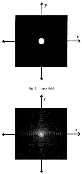
In this work, the scalar optical diffraction is obtained by using the plane wave spectrum approach [IO], [12]. The simulator has two parts. First part takes an image which is in raw format, and converts it to a complex data matrix. The obtained matrix is become our input field of which diffraction field will be calculated. An example of an input can be seen in figure 2. Second part calculates the diffraction pattern of the object on a predefined plane in the space.

11. MATHEMATICAL MODEL

The scalar diffraction theory for monochromatic coherent light is formulated not only in the spatial domain but also in the frequency domain [6]. In this work we deal with the latter case. Fourier analysis of the input field provides the complex amplitudes of the plane waves which propagate in different

directions. We can represent the relation between a given field over two-dimensional plane, A( IC,, ICy), and three-dimensional field in space, $(z, y, z ) , as

$(z, y,

z )

= / A ( I C , , / c , ) e j ( k r " + k Y y )

dlc,dIC,. (1)

e3 J k 2 - k r 2 - k V 2 z

Moreover, we replace z = 0 into equation (I), we obtain the field on a reference plane z = 0 and it is shown as

f(z, y) $(z, y, 0 ) = / A ( & , ky)e3(k~s"+k~Y)dIC,dICy. (2)

We observe from equation (2) that A(S,, ICy) is equal to the Fourier transform (FT) of the field on

z

= 0 plane.

We define

z

= 0 plane as the input plane which is shown in figure 2. The input plane is spanned by 2 = (1,0,0) and

= (0,1,0) unit vectors. The plane contains the diffraction field, which is called as the observation plane, is represented by

2=RRZ+G

(3)

where R is a rotation matrix and

6

is the trans!ation vector in space. The observation plane is spanned by z' = R5 and

y' = Ry vectors. Moving on input plane provides tracing on observation plane and it is shown in equation (3). By the substitution of equation (3) in equation (I), we obtain the diffraction field on the observation plane as

H ( 2 , R, G)J(lc,, IC,')dkkdIC& (4)

where = Rl? and IC' represents the propagation of the plane waves according to the observation plane. The function

J ( k , , ICz') is the Jacobian and equals to

$

[lo]. Please note that IC; is a function of IC; and

IC&.

Since

i h 2

+ ICh2 +

lcL2 =

9.

Moreover, ICz is function of IC;, IC' and

IC;

through the relationship = RQ. The function H(IC', R,

G)

provides the kernel of the system and represented as

y ,

H ( 2 , R,

g)

= e j c T ( R T g ) . ₍₅₎

0-7803-8379-6/04/$20.00 02004 IEEE.

(2)

The relation between f ( x , y) and g(z, y) can be obtained from equations (2) and (4) as

H ( p , R , G ) k . )

( 6 )

where F(k,, ky) is the FT of the f ( z , y). Please note that 47r2 and &terms cancel each other and therefore not necessarily needed for the implementation of the algorithm.

111. DISCRETE MODEL

Discrete model of the system, which represents the scalar optical diffraction, is obtained by sampling equations (2) and (4). Since sampling a signal in space domain causes replications in its frequency domain representation, and vice versa, we deal only with periodic inputs and output. The implemented simulator displays only one period of the input and the output. By sampling the space and the frequency domains, we obtain

x

= Xn,, y = X m , ,

(7)

where X is the sampling period. N shows the size of the frame we deal with. The discrete variables n,, m,, n; and m; are integer numbers in the range [-N/2, N/2) [12], [13]. The discrete version of kk is

where

P

is equal to

y.

The variables

IC;

and kh are uniformly sampled. Hence the angle between the consecutive plane wave components, as represented

9

the corresponding

k;',

which is the discrete version of k', becomes larger as the wave vector of the plane wave moves away from the observation-plane normal. Therefore there is a non-uniform sampling in k domain. This nonuniform sampling affects the weights of the samples in such a way to cancel the Jacobian in equation (4). Therefore, the Jacobian in equation (4) vanishes in the discrete version. The discrete simulation of the model is performed by the steps indicated below:

An N x N input array is given by the user (An example is shown in figure 2). This array represents the samples of a periodic f ( z , y) which are taken in the range (x,y)e[-,

y).

Then, an N x N array fD(n,,m,) is created which corre- sponds to samples in the range (2, y)e[O, N X ) of f

(x,

y) by

periodically shifting the given input, accordingly. After that

where (n;,m;) is in the range

[F,

g)

and u(n;,m;) and

v(n;, m;) are computed as

u(n;,

m;)

=

(n;

+

S ) T 1 1

+

(m'f

+

t ) m

+J,P

- ( n l f

+

s>2 - (m'f

+

t ) 2 r 2 3 (1 1) where s , t are chosen to be equal to ~ 3 1 0 and r32P, respec-

tively. This operation is needed to compute A ( R k ' ) given in equation (4). The rotation matrix is defined as

r11 T 1 2 r13

R =

(;;;

;;;

%)

(12)

P is a function obtained from

A ~ ( n f ,

m f ) by bilinear interpolation. The nearest 4 pixels to the location indicated by

u(n;,

mi),

w(n;,

m;) are used in the bilinear interpolation

The function f ( z , y) usually represents a base-band signal. Therefore, the frequency components of A(k,, k y ) are con- centrated around the origin. The transformation k' = R-lrc'

yields conversion of the concentration in equation (4) from around ( k z , k y ) = (0,O) to around ( k ; , k h ) =

( T ~ I P , T ~ ~ P ) .

Therefore, the signal in equation (4) whose inverse FT (IFT) is going to be taken, is usually a band-pass signal. To avoid unnecessarily large discrete FT (DFT) sizes, the band-pass signal is converted to a base-band signal by introducing the s and

t

in equation (1 1) during the dmrete computations. Please note that u(n;, m;) and v(n' m' ) are no longer integers for integer n;, m;. Then H D ( ~ ' , R, b ) is defined which is the

discrete version of the kernel in equation ( 5 ) and it is given as (1 3 )

f '

f , 2 r k>'. 6

~ ~ ( 2 ,

R,

b'>

= e m - T where k~

discrete form of equation (4) is obtained as

equals to ( n f , m f ,

Jp2

- n f 2 - m f 2 ) . Thus the

N - 1

g D ( n S , m S )

'

A 1 , D ( n ; 7 m ) ) n;?m;=O

(14)

,j

%

(n,n;+m,m;)H D ( P , R,

G).

The function gg(n,,m,) is the discrete form of +(R(z, y, O)T

+

b ) . Consequently, the relation between

f ~ ( n , , m,) and gg(n,, m,) is given as

1 N2

g g ( n s , m,) = --DFT-l{A1,~(n;, m;)Ho(G', R,

G)}.

(15) Please note that N2 in equation (9) and

&

in the above equation cancels each other- and therefore they are not needed during the implementation.

IV. SIMULATION RESULTS

A computer simulation was carried out, and the algorithm used can be summarized as follows. A two-dimensional input array is generated or given by the user. The gray levels of (9)

function

(10)

(3)

the pixels represent the field strength. Due to discretization, the input array represents a rectangularly periodic optical field with a period N X . Then A l , ~ ( n ; , r n ; ) is calculated as described in equation (10). After that, the discrete kernel of the system is obtained by using equation (1 3). Inverse DFT (IDFT) gives the scalar optical field on determined observation plane and we display its magnitude.

The illustration of the implemented scenario is given in figure 1. In the simulations, the input is a 256 by 256 matrix. Therefore, N equals to 256. Computations are carried out using double precision arithmetic (4 bytes for the real and four bytes for imaginary parts of each pixel). Each pixel of the field is represented by 8 bytes. The variables of implemented model depend on A. Therefore, changing X causes some changes in physical values of the other parameters. In this simulation, it is assumed that the wavelength is taken as 633nm. In the given simulations the sampling period is cho_sen as 2X, therefore, ,O becomes 512. The translation vector b is chosen as (0,0,0.166) meters. The presented results in the figures correspond to 0, 15, 30, 45 and 60 degrees rotation around the y-axis. Moreover to improve the visibility of the peripheral fringes, we chose to display

d m - .

V. CONCLUSION

Plane wave spectrum approach provides a fast numerical method for Rayleigh-Sommerfeld diffraction integral; there is no need for Fresnel and Fraunhofer approximations. The presented model and the associated simulations are for the monochromatic case. In our simulations, the direction of propagation is limited to be the along the positive z-direction; this fits well for most of the applications. If desired, this restriction can be easily removed. As usual in digital simulations, the results correspond to periodic input structures; in order to minimize the effect of the periodicity, larger DFT sizes which can accommodate the diverging diffraction pattern sizes are recommended. The simulator results are satisfactory.

REFERENCES

[ I ] L. Onural and P.D. Scott, ”Digital Decoding of In-line holograms”, Opt. Eng., vol 26, no 11 pp 1124-1 132, Nov 1987.

i‘

Y

‘,dy

Observation Plan1

Fig. 1. Illustration of the implemented scenario

r”

.L

Fig. 2. Input field

T

Fig. 3.

which has no rotation around y-axis

Square root of magnitude of diffracted field on observation plane

G. Bozdagi, ”Simulation of a holographic 3-D television display”,

Ms Thesis, Electrical and Electronics Engineering and Institute of Engineering and Sciences of Bilkent University, 1990.

S. Ganci, ”Fourier diffraction through a tilted slit”, Eur. Phy. 2, 158-160,

1981.

K. Patorski, ”Fraunhofer diffraction pattern of tilted planar objects”, Opt. Acta 30 673-679, 1983.

H.J. Rabal, N. Bolognini and E. E. Sicre, ”Diffraction by a tilted aperture, coherent and partially coherent cases”, Opt. Acta 32, 1309- 1311, 1985.

J.W. Goodman, ”Introduction to Fourier Optics”, McGraw Hill, New York, 1968.

D. Leseberg and C. Frere, ”Computer generated holograms of 3-D objects composed of tilted planar segments”, Appl. Opt. 27, 3020-3024,

1988.

C. Frere and D. Leseberg, ”Large objects reconstructed from computer- generated holograms”, Appl. Opt. 28, 2422-2425, 1989.

D.K. Cheng, ”Field and Wave Electromagnetics”, chapter 8, Addison- Wesley.

T. Tommasi and B. Bianco, ”Frequency analysis of light diffraction between rotated planes”, Opt. Lett. 17, 556-558, 1992.

(4)

T

Fig. 4.

which has 15 degrees rotation around y-axis

Ty

Fig. 5.

[ 1 13 T. Tommasi and B. Bianco, ”Computer-generated holograms of tilted planes by a spatial frequency approach”, J. Opt. Soc. Am. A IO, 299- 305, 1993.

[I21 N. Delen and B. Hooker, ”Free-Space beam propagation between arbitrarily oriented planes based on full diffraction theory: a fast Fourier transform approach”, J. Opt. Soc. Am. A, vol 15, no 4, pp. 857-867, Apr. 1998.

1131 N. Delen,”Plane wave spectrum treatment of tilted and offset planes by using a new FFT based method”, PhD Thesis, Department of Electrical and Computer Engineering of University of Colorado, 2000.

[14] B.E.A. Saleh and M.C. Teich, ”Fundamentals of Photonics”, chapter 4, John Wiley and Sons Inc, 1991.

T

Fig. 6.

T’

Fig. 7.