Abstract— Additive manufacturing has become increasingly popular for a wide range of applications in recent years. Micro-stereolithography (µSLA) is a popular method for obtaining polymer-based parts. Systems using the µSLA approach usually consist of a vertical positioning system, a light source and a container where the component is built gradually as the polymer is cured at the locations where the ultraviolet light is projected. It has been noted that the motion of the positioning system and the intensity of the light source is an important factor to achieve high level dimensional precision. In this paper a three dimensional error based learning scheme is presented to improve the time varying process parameters of the system so that the dimensional accuracy of the product is improved. A mathematical model of the curing process is used for developing the error based learning algorithm. The current process parameters as a function of time and the dimensional error obtained at each layer of the production are used for increasing the quality and precision of the same part in the next iteration. Our initial simulation results show significant improvements can be obtained in a few iterations if the correct learning parameters are used based on the target parts dimensional properties.
I. INTRODUCTION
The process of projection micro-stereolithography is a complex manufacturing technique with the interaction of various scientific areas. It includes chemistry as UV-curable materials are used and since the process is based on photo-polymerization [1]. Principles of optics are also important because of the light projection on the resin surface. The motion of the production platform plays an important role due to the adequate curing time and inertial effects on the part. The complexity of the system results in many process variables that must be selected first to obtain acceptable products. Development of process planning schemes is a common research area in which process parameters are associated with the manufactured part geometry to reach accurate structures when compared to the desired part design [2]. Tolerances could be decreased as the photo-polymerization affects the surface finish and geometrical accuracy is observable through detailed measurements at
*This research is sponsored by Scientific and Technical Research Council of Turkey (TUBITAK) through Project No: 113M172.
E.B. Türeyen is with the Mechanical Engineering Department, İ. D. Bilkent University, Ankara, 06800, Turkey (e-mail: [email protected]).
M. Çakmakcı is with the Mechanical Engineering Department, İ. D. Bilkent University, Ankara, 06800, Turkey (phone: +90 312-290-34-27; e-mail: [email protected]).
Y. Karpat is with the Mechanical Engineering and Industrial Engineering Departments, İ. D. Bilkent University, Ankara, 06800, Turkey (e-mail: [email protected])
micron level accuracy [3]. However, over-curing or
stair-stepping effects may result in products with bad dimensional
accuracy.
Gray-scale pixel planning and intensity variation is used as a novel approach to decrease the effect of the meniscus shape caused by the step-by-step movement [4]. It is observed in the previous research that even if the machine itself is optimized for best dimensional performance based on the best subsystem settings, the dimensions and features of the product that is targeted also affects the quality of the end product. In order to decrease the total manufacturing time and increasing the quality of the parts without making large number of trials for process variables a more structured approach is required.
Control of the UV light based layer-by-layer curing is also a field that researchers have been studying in recent years. In [5], model of a hybrid system consisting layering and curing, for creating an optimization scheme of the process was studied with a stepped motion. Optimal conditions for both inter-layer hold times and UV intensity of the source are found using the model and application on the simulations. Most of the current control schemes are based on open-loop process control for micro-fabrication with projection lithography. In [6], an Evolutionary Cycle to Cycle (EC2C) control scheme and a dynamic model with adaptive neural network back-stepping was developed to control the exposure time and light intensity.
In this paper a three dimensional error based learning scheme is presented to improve the time varying process parameters of the system so that the dimensional accuracy of the product is improved. A mathematical model of the curing process is developed and then used for developing the error based learning algorithm. The current process parameters as a function of time and the dimensional error obtained at each layer of the production are used for increasing the quality and precision of the same part in the next iteration.
The outline of the remaining of the paper can be given as follows. In section 2, our current system setup is discussed. In Section 3, a mathematical curing model, developed based on our system and the learning algorithm based on the dimensional errors are given. In Section 4, the simulations based on the mathematical model and the iterative learning algorithm is presented. Our current conclusions and future work is discussed in Section 5.
Development of an Iterative Learning Controller for Polymer based
Micro-Stereolithography Prototyping Systems*
E.B. Türeyen, Y. Karpat and M. Çakmakcı
Boston Marriott Copley Place July 6-8, 2016. Boston, MA, USA
II. ADDITIVE MANUFACTURING USING MICRO-STEREOLITHOGRAPHY
A. A. Setup
Stereolithography is the process in which a photo-curable liquid resin is exposed to UV light and gets solidified. Resin layer, the portion between the top surface of the resin vat and moving platform floor (Fig. 1), is cured as the first layer of the structure, using the projected layer image based on the layer image data developed from the CAD model of the product. After the curing of first layer, fabrication platform is lowered vertically in the amount of the selected layer thickness and image of new layer is projected. As the platform movement progresses, the target three-dimensional product is created using the sliced layer images of design.
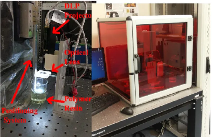
In Fig. 1, developed Projection based Micro-Stereolithography Prototyping device and the system setup with the components are shown. A DLP projector is used in the setup as the UV light source. The setup and position control algorithms used in the system was presented in [8, 9]. Positioning system is used to locate the production platform on the top side of the resin with leaving a small layer of liquid above the platform, which will then be cured as the first layer. Normally, light rays coming out of the DLP projector diverges and decreases the resolution of the image on the production surface. For increasing resolution and creating micro dimensional structures, a converging aspheric lens is used to collect the light. A CAD model slicing software is used to create the layer-based images and project them in the order of process. An enclosure is assembled to decrease the effect of outer light sources to the process and also to protect the manufacturing area.
B. B. System Parameters and Variables
The µSLA fabrication device developed, works based on certain parameters and process variables that needs to be selected to operate its sub-systems. Some of these values come from the chemical composition of the UV-curable resin. The critical curing energy and depth of penetration for the resin are important parameters in the modelling of the process for the liquid polymer structure. UV-spectroscopy is performed to identify these parameters.
For the projector, the amount of the irradiation is calculated using a power-meter. Then, the measured amount of energy taken at a specific distance is used for the exposure calculation for the mathematical model. Value of irradiation could be changed in a specific interval using the controller of the device. Apart from the subsystems, parameters that are used for the fabrication process are the layer thickness (or the number of layers) and the exposure time for the production. The number of layers varies according to the original height of the part and the layer thickness.
C. C. Cure Depth Mathematical Model
In order to develop advanced algorithms to improve the quality of products done with micro-stereolithography, realistic models of the process that helps to understand the curing (solidifying) are needed.
Figure 1. System setup and its protective enclosure
Beer-Lambert law [7] provides the mathematical explanation to the chemical process of movement and decay of the incoming light rays in a material that it travels through. Attenuation of the light rays as they enter the liquid causes a variance in the manufactured shape. Logarithmic exposures relation with the critical curing energy makes it possible to calculate amount of curing in photo-active resin.
Calculation of the curing depth caused by the attenuated light inside the resin is the basis of the mathematical model and simulations used for this research. Beer-Lambert law is used with the polymer resin curing process when the formula is modified to calculate the amount of attenuated light for a desired location inside a liquid with given properties [1]. Therefore, a layer cure model is created that can calculate the amount of curing for a given area in the liquid polymer resin. One of the most important parameters that shape the characteristic of the resin is the cure depth, which explains the depth of solidification with a specific amount of energy. In [7], cure depth is given in the “standard design equation” of stereolithography as follows:
Cd = Dp ln (E / Ec) (1) Where, Cd is the calculated cure depth for the resin, Dp is the depth of penetration which is a material constant that resembles the penetration of light inside the liquid structure. Ec is the critical energy of the resin which has a crucial role in the cure depth model as only in the areas where the exposure is larger than the critical energy, the curing occurs. Exposure value, E, so called to light irradiation dose, used in the calculations defines the total irradiation, I, created on the resin surface for a given period of time in terms of mJ/cm2.
E (mJ/cm2) = I (mW/cm2) * t (sec) (2) For finding the exposure amount on the surface, measurements are done based on the calculation of un-calibrated area exposure observed with the DSLR camera images. By averaging the color intensity values of every pixel in Matlab, result is compared to the power-meter light intensity value previously found and calibrated pixel exposure amounts are calculated.
Using a specific image and dimensions, average irradiation is found as 30.6 mW using a power-meter. Area
of the projected shape on the surface is 4.16 cm2 so the irradiation on the unit area is calculated as 7.394 mW/ cm2 (2). Depth of penetration value is found with the help of Fourier Transform Infrared Spectroscopy made on the prepared liquid polymer. The test gave the transmittance amount of light inside the resin for varying wavelengths. In (3), T represents the amount of transmittance (3), where ɛ is the attenuation coefficient and l is the thickness of the measured sample in the test.
T = e-ɛl (3) Using the attenuation constant, penetration depth of the liquid is found as shown in (4).
Dp = 1/ɛ (4) From the results of the FTIR, the blue light area with the wavelength of 460nm is taken into consideration as resin starts curing in this interval. Transmittance at that wavelength is %81, so Dp for the resin is found as 96.936 µm/s.
In [10], the primary formula of the model used to estimate the amount of curing for a single point given the exposure at a specific depth of z is shown in (5)
Ez = E * e -z / Dp (5) For our system the critical energy is found through an experimental method and productions are done in order to reach the exact value. Cure depth formula [11] is re-arranged and as all other parameters are known, an experimental method is used to find the critical energy. (1) Resultant value for the energy is calculated as 7.266 mJ/ cm2.
III. ITERATIVE LEARNING ALGORITHM
Fig. 2 shows the overall block diagram of the µSLA System and how the exposure time based learning algorithm and the vertical position controller of the system interacts. As there reference shape is analyzed the structure interpreter determines each layer shape and the layer thickness height. The layer shape is sent to the light source (i.e. the DLP projector) and based on the desired layer thickness desired position data is fed on the position controller.
For smooth operation and near layerless production position controller uses the information and the current position to calculate a desired velocity for the platform. Then in the conventional operation the actual velocity of the platform is compared to the desired value and new control command is calculated based on the velocity controller. Continuous movement causes the exposure time to be only adjusted by the platform velocity. When learning algorithm is activated, the algorithm uses the desired layer image and the actual layer image data from the previous iteration to calculate a dimensional error of the structure. Based on the error at the previous and upcoming layers, the algorithm calculates a correction term that speeds up or slows down the motion of the platform for less exposure time or more exposure time at the layer respectively. The correction trace calculated after each iteration is given as shown in (6).
Figure 2. µSLA System Block Diagram
N M j i layer i ovr i il ze
k
j
N
M
k
v
k
v
(
)
1
)
(
)
(
)
(
1 1 ,
(6)Where,
v
iz,il(
k
)
is the correction trace, k is the time step)
(
1k
v
iovr is the desired velocity input from the previous iteration number i-1, γ is a learning gain and
e
layeri1(
k
)
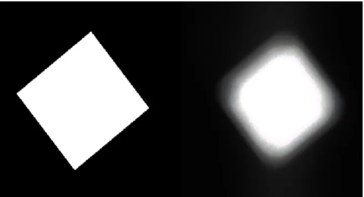
is two dimensional shape the error for the layer corresponding to the time step k. Error is calculated as an average of the previous M and next N layers as exposure is incremental on every layer and causing the error of over-curing.The reflected layers image on the manufacturing surface is used as another input for the learning algorithm. A reference layer description that defines the desired structure is created. That reference structure is based on the perfect reflected shape on the production platform which is named as the desired layer shape in Fig. 3 on the left side. That reference image is firstly used to create a 3D structure using the simulation.
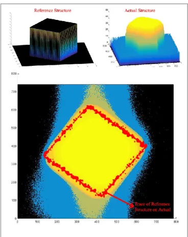
Because of the variations in the formation of the light on surface, caused by the errors of the optical system and outer light effects, the projected image on the surface never reaches the exact specifications when compared with the desired irradiation amount for each pixel as shown in Fig. 3 on the right side. Layer images reflected through the projector and the optical system, are recorded on the fabrication surface using a CCD camera, for being used as an input in the mathematical simulations. This image is called as the actual layer image. The average profiles of these images are given in Fig. 4.
Figure 4. Initial simulation results showing actual and reference structures IV. SIMULATIONS
In order to test our algorithm in a controlled environment a simulation study is performed on the mathematical modelling of the photo-polymerization process using the previously defined cure model and the learning algorithm defined in (6).In order to apply the algorithm, the error calculation process starts by comparing the actual structure and reference model as shown in Fig. 5 for each layer. For the first layers, every pixel value is compared between the two structures to observe the differences. That creates an error value for the clear observation of the comparison which will be useful for the next steps of the algorithm.
Figure 5. Irradiation image profiles
If the actual model includes a cured pixel but the reference does not, a negative error value is assigned for that point which means that there is over curing on that area and it is recurred for each pixel. Therefore, an error value for that layer is generated to be used in the
e
layeri1(
k
)
term. This operation is done for all layers one by one. Then the accumulated value of the production error is also considered for the whole production, to be used in the performance comparison. The overall desired velocity command was also recorded as a function of time for each production to be used in the next iteration as part of the learning algorithm.In the next iteration, with the use of new values, new exposure quantities were determined and actual structure is produced again in the simulating environment. In all iterations, new error values are found and time parameter is changed for decreasing the amount of error using the simulations. Our objective is to obtain nearly optimal variation of parameters for all layers of the designed part in small number of iterations. To standardize the process, layer thickness, layer number and exposure amount is kept constant in all trials. Simulations are done for 1 µm layer thickness and total of 50 layers. Used DLP projector is capable of changing the light intensity by adjusting the amount of current given to the LEDs. Irradiation is based on the light intensity of the projector. Therefore, intensity is kept the same for all trials to not affect the exposure by changing the irradiation. That ensures that the control flow given in Fig. 2 is followed. Even though the negative and positive error values are differentiated for describing over and under curing, same correction weight is used for both of them. Also using the absolute value of the over-curing and adding it to the under-curing error, a total error amount is calculated. All error amounts are expressed by the under-cured or over-under-cured pixels according to the reference model. Total pixel amount for 50 layers is close to 30 million pixels. First design for the simulation is taken as a cubic shape in order to observe the effectiveness of the system in a basic shape and to measure the magnitude of error easily. A secondary and more complicated shape is used and tested to control the scheme and observe whether the baseline settings found are applicable for varying more complex geometries.
A. A. Basic Shape
Using the previously defined parameters, a cubic shape is tackled as the first project. Number of iterations is kept constant at 5 for comparison. Various correction factors are tested in initial simulations also with changing the first exposure time. Before the initial learning trials, simulations are run to visualize the resultant 3d structures of the desired and actual images with a single exposure time value for every layer. (Fig. 4) Simulations are done with 4 different starting exposure times. 1, 1.4, 1.6 and 2 seconds are chosen and errors are calculated for 3 different correction coefficients. It is observed that after 5 iterations, error is decreased to %40 of the initial amount. (Fig. 6) Starting from the first error calculation, the parameter changing algorithm for correcting the exposure time amount for layers, works efficiently.
Figure 6. Variation of error with new iterations according to changing correction factors
The exposure time variation at the end of iterations is showed as a function of layer number which is directly correlated to the platform speed vz at constant layer thickness. (Fig. 7) After starting with a single exposure time, nearly all exposure times for 50 layers are adjusted to different values in the second iteration. Algorithm executes the learning of the correct exposure time according to the value of the error so when the error decreases to zero, it starts keeping the exposure time the same.
Results in Fig.6 showed that, for the starting parameter of 1 second exposure time, best results converged to the correction factor of 1*10-6. Using this coefficient to multiply with the previous error of a layer and sum up with the time, total structural error decreased %42 percent when compared to the initial error.
The learning algorithm is trying to decrease huge amount of errors especially in the nearly totally over-cured first few layers. Effectiveness could be increased if the base idea of this work is revisited again. Cure depth calculation is working according to Beer- Lambert Law, which states that even though light vanishes after a specific depth because of attenuation, until reaching that depth, the total exposure increases on all layers that light passes through. It can be assumed that when the error amount of a layer is examined and it is over-cured, the over-exposure of that layer is also increasing the irradiation amount of the pixels underlying it.
Figure 7. Variation of exposure time for layers in 5 different iterations
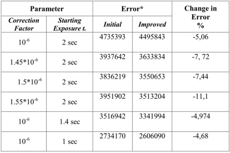
Therefore, learning algorithm parameters M and N can also be changed instead of taking the single layers error into account and multiplying it with correcting coefficient, an average of that layer and the 4 other underneath it is taken into account and used in the calculations. A similar logic is driven for the under-cured layers. As the error in a less irradiation applied area is also suffering from the lack of irradiation of the layers over it, the error amount of the ones located above also adds up in an average and makes the algorithm create sharper increases in the exposure time. With the new adjustment the results in Table 1 shows that, according to the first algorithm with the same correction factor, an additional decrease up to % 11 in error is reached, again with 5 iterations.
TABLE 1. Error Decrease with the iterative algorithm Parameter Error* Change in
Error % Correction
Factor Exposure t. Starting Initial Improved
10-6 2 sec 4735393 4495843 -5,06 1.45*10-6 2 sec 3937642 3633834 -7, 72 1.5*10-6 2 sec 3836219 3550653 -7,44 1.55*10-6 2 sec 3951902 3513204 -11,1 10-6 1.4 sec 3516942 3341994 -4,974 10-6 1 sec 2734170 2606090 -4,68
* Error amount is given in the amount of wrongly cured pixels for all layers
B. B. Validation with a Complex shape
As mentioned before, also a more complex shape is put under test to verify the contribution of the learning scheme. A cross shape is used which has a curvy structure and small angled edges as shown in Fig. 8. Simulations with different coefficients showed that, algorithm is also valid for decreasing the amount of the error at the end of 5 iterations. Exposure model of that shape had a major difference when compared to the first shape, because the over illuminated areas can be observed easily (Fig. 8). Also the irradiance variation and the scattering of the light intensity profile are extremely high. The reason of that intensity variance is caused by the four thinner areas of the cross shape.
Figure 8. Reference image on the left versus actual image on the right 0 2000000 4000000 6000000 8000000 10000000 12000000 1 2 3 4 5 Er ro r Iteration 1.45*10^-6 1.5*10^-6 1.55*10^-6
Correction
Factor
Figure 9. Simulation results showing reference and actual structures That structure made the center area brighter but the thin parts less illuminated. Even though thin parts seemed darker, sizes are similar to the reference model. That resulted in more over-curing and high amount of error for the algorithm to figure out in the starting iteration. (Fig. 9) But as the error is only formed in the negative side, it made the algorithm work mode stable.
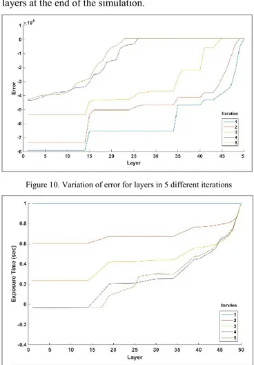
With the use of the improved algorithm, error correction scheme gave around %79 improvement on the surface shape quality with the optimum algorithm and process parameters as shown in Fig. 10 with one second of initial exposure time and 5*10-6 as the error correction factor. In Fig. 11, variance of exposure time for layers shows how the algorithm adjusts the exposure in iterations for reaching the zero error for 28 layers at the end of the simulation.
Figure 10. Variation of error for layers in 5 different iterations
Figure 11. Variation of exposure time for layers in 5 different iterations
V. CONCLUSION
In this paper an iterative learning algorithm that will adjust micro-stereolithography process parameters so that the pixel curing error is minimized. That adjustment is done with comparing the simulation results based on the mathematical modelling of the system, to the reference model. For two different shapes, dimensional error of the final product are decreased up to %80 compared to the constant parameter based simulations. Although variation in the error performance exists, results of the complex structure simulations showed that, improvements on the algorithm could be made to decrease the error value even more, for the effective usage in varying structures.
Next step of this work is the experimental application of the model and learning algorithm on the introduced setup, with also improving the structure of the learning algorithm to include the light intensity variations.
ACKNOWLEDGMENT
Authors would like to thank Mr. Zulfiqar Ali for his work and valuable contributions in the development of the stereolithography system setup.
REFERENCES
[1] Sun, Hong-Bo, and Satoshi Kawata. "Two-Photon
Photopolymerization and 3D Lithographic Microfabrication." NMR
3D Analysis Photopolymerization Advances in Polymer Science, 2004,
pp. 169-273.
[2] Lynn-Charney, Charity, and David W. Rosen. "Usage of Accuracy Models in Stereolithography Process Planning." in Rapid Prototyping
Journal 6.2, 2000, pp. 77-87.
[3] Stampfl, J., S. Baudis, C. Heller, R. Liska, A. Neumeister, R. Kling, A. Ostendorf, and M. Spitzbart. "Photopolymers with Tunable Mechanical Properties Processed by Laser-based High-resolution Stereolithography." J. Micromech. Microeng. Journal of
Micromechanics and Microengineering 18.12: 125014, 2008.
[4] Pan, Yayue, Xuejin Zhao, Chi Zhou, and Yong Chen. "Smooth Surface Fabrication in Mask Projection Based Stereolithography."
Journal of Manufacturing Processes 14.4, 2012, pp. 460-70.
[5] Yebi, Adamu, and Beshah Ayalew. "A Hybrid Modeling and Optimal Control Framework for Layer-by-layer Radiative Processing of Thick Sections." in 2015 American Control Conference (ACC), 2015.
[6] Zhao, Xiayun, and David W. Rosen. "Process Modeling and Advanced Control Methods for Exposure Controlled Projection Lithography." 2015 American Control Conference (ACC), 2015.
[7] Jacobs, Paul F., and David T. Reid. Rapid Prototyping &
Manufacturing: Fundamentals of Stereolithography. Dearborn, MI:
Society of Manufacturing Engineers in Cooperation with the Computer and Automated Systems Association of SME, 1992.
[8] Nurcan Gecer-Ulu,, Erva Ulu,, Çakmakcı, M. "Design and Analysis of
A Modular Learning Based Cross-Coupled Control Algorithm for Multi-Axis Precision Positioning Systems", International Journal of
Control Automation and Systems, 2016, v.14(1)
[9] Erva Ulu,, Nurcan Gecer-Ulu,, Çakmakcı, M. "Development and
Validation of an Adaptive Method to Generate High-Resolution Quadrature Encoder Signals", Journal Dynamic Systems
Measurement and Control, 2014, v.136(3) p.034503
[10] Lee, Jim H., Robert K. Prud'homme, and Ilhan A. Aksay. "Cure Depth in Photopolymerization: Experiments and Theory." Journal of
Materials Research J. Mater. Res. 16.12, 2001, 3536-544.
[11] Limaye, A.s., and David W. Rosen. "Process Planning Method for Mask Projection Micro-stereolithography." in Rapid Prototyping