3D reconstruction of point clouds using multi-view orthographic projections

(1)

3D RECONSTRUCTION OF POINT CLOUDS

USING MULTI-VIEW ORTHOGRAPHIC

PROJECTIONS

A THESIS

SUBMITTED TO THE DEPARTMENT OF ELECTRICAL AND ELECTRONICS ENGINEERING

AND THE INSTITUTE OF ENGINEERING AND SCIENCES OF BILKENT UNIVERSITY

IN PARTIAL FULFILLMENT OF THE REQUIREMENTS FOR THE DEGREE OF

MASTER OF SCIENCE

By

Osman Topçu

(2)

I certify that I have read this thesis and that in my opinion it is fully adequate, in scope and in quality, as a thesis for the degree of Master of Science.

__________________________________ Prof. Dr. Levent Onural (Supervisor)

__________________________________ Prof. Dr. Ergin Atalar

__________________________________ Assistant Prof. Dr. Selim Aksoy

Approved for the Institute of Engineering and Sciences:

__________________________________ Prof. Dr. Mehmet Baray

(3)

ABSTRACT

3D RECONSTRUCTION OF POINT CLOUDS USING

MULTI-VIEW ORTHOGRAPHIC PROJECTIONS

Osman Topçu

M.S. in Electrical and Electronics Engineering Supervisor: Prof. Dr. Levent Onural

June 2006

A method to reconstruct 3D point clouds using multi-view orthographic projections is examined. Point clouds are generated by means of a stochastic process. This stochastic process is designed to generate point clouds that mimic microcalcification formation in breast tissue. Point clouds are generated using a Gibbs sampler algorithm. Orthographic projections of point clouds from any desired orientation are generated. Volumetric intersection method is employed to perform the reconstruction from these orthographic projections. The reconstruction may yield erroneous reconstructed points. The types of these erroneous points are analyzed along with their causes and a performance measure based on linear combination is devised. Experiments have been designed to investigate the effect of the number of projections and the number of points to the performance of reconstruction. Increasing the number of projections and decreasing the number of points resulted in better reconstructions that are more similar to the original point clouds. However, it is observed that reconstructions do not improve considerably upon increasing the number of projections after some number. This method of reconstruction serves well to find locations of original points.

Keywords: 3D reconstruction, visual hull, shape from silhouettes, volumetric intersection,

(4)

ÖZET

NOKTA BULUTLARININ ÇOK YÖNLÜ ORTOGRAFİK İZDÜŞÜMLERİNDEN GERİ ÇATMALARININ ELDE EDİLMESİ

Osman Topçu

Elektrik ve Elektronik Mühendisliği Bölümü Yüksek Lisans Tez Yöneticisi: Prof. Dr. Levent Onural

Haziran 2006

Üç-boyutlu nokta bulutlarının ortografik izdüşümlerinden geri çatmalarının elde edilmesine yönelik bir yöntem sınandı. Nokta bulutlarını oluşturmak için rasgele süreçler kullanıldı. Nokta bulutlarının meme dokusunda bulunan mikrokalsifikasyon oluşumunu modellemesi için rasgele süreçler tasarlandı. Nokta bulutları bir Gibbs örnekleme algoritması kullanılarak oluşturuldu. Nokta bulutlarının istenilen yönlerden ortografik izdüşümleri elde edildi. Elde edilen ortografik izdüşümlerden nokta bulutlarının geri çatmalarını elde etmek için hacimsel kesişim yöntemi uygulandı. Ortaya çıkan nokta bulutlarının geri çatmalarında hatalı noktaların oluşabildiği gözlendi. Bu hatalı noktalar, oluşma sebeplerine göre sınıflara ayrılarak, doğrusal birleşime dayanan bir performans değerlendirme ölçütü belirlendi. İzdüşüm ve toplam nokta sayısının performansa etkisinin araştırılması için deneyler tasarlandı. İzdüşüm sayısının arttırılması ve toplam nokta sayısını azaltılması gerçek nokta bulutlarına daha çok benzeyen geri çatmalar ortaya çıkmasını sağladı. Fakat izdüşüm sayısının arttırılmasının bir noktadan sonra performansa fazla bir etkisinin olmadığı anlaşıldı. Bu geri çatma yöntemi nokta bulutlarını oluşturan noktaların yerlerinin belirlenmesi için kullanılabilir.

Anahtar Kelimeler: Geri çatma, görsel zarf, silüetlerden şekillendirme, hacimsel kesişim, nokta bulutları, Gibbs örnekleyicisi, ortografik izdüşüm

(5)

ACKNOWLEDGEMENT

I would like to thank to my family for their constant support.

This work is partially supported by EC within FP6 under Grant 511568 with the acronym 3DTV.

(6)

LIST OF FIGURES

Fig. 1. Perspective projection Fig. 2. 3D discrete lattice structure

Fig. 3. Digital mammography image illustrating microcalcifications in breast tissue Fig. 4. Single-voxel clique and examples of two-voxel cliques

Fig. 5. Rubik’s cube to illustrate 26-neighborhood

Fig. 6. Illustration of Gibbs Sampler algorithm in 2D using a 3 by 3 square white region

surrounded by black region. a, b, c, d, e, f indicate changes in each step of the iteration

Fig. 7. Orthographic projections of three points in space Fig. 8. Cross-section of projection planes and point clouds Fig. 9. Parallel discrete lines

Fig. 10. Figure illustrating 4-neighborhood and 8-neighborhood Fig. 11. Continuous line in a 2D discrete lattice

Fig. 12. Orthographic projection of point clouds

Fig. 13. Orthographic projection of point clouds from different viewpoint Fig. 14. Convex and non-convex sets

Fig. 15. A line segment, a triangle and a tetrahedron Fig. 16. A set of points in plane and their convex hull Fig. 17. Convex hull of a polyhedron in space

Fig. 18. Traffic signs

Fig. 19. Illustration of volumetric intersection method. Squares are swept to generate the

cube

Fig. 20. Reconstruction of 2 points using 2 image planes Fig. 21. Reconstruction of 2 points using 3 projection planes Fig. 22. Two digital lines intersecting in more than one pixels Fig. 23. Intersection of right angled lines

Fig. 24. Ray directions indicating orientation of projection planes that are used to

(8)

Fig. 25. A frame of video file displaying the original data on the left and the

reconstructed data on the right side

generate the reconstruction displayed in Figure 27

Fig. 27. Another frame displaying both the original and the reconstructed data Fig. 28. Ray directions indicating orientation of projection planes that are used to

Fig. 29. Video frame showing original data and its reconstruction

Fig. 30. Frames 76, 77, 78, 79, 83 of output video. Three projections whose ray directions

are shown in Figure 24 are used in this reconstruction.

Fig. 31. Frames 76, 77, 78, 79, 83 of output video. Four projections whose ray directions

Fig. 32. Frames 76, 77, 78, 79, 83 of output video. Five projections whose ray directions

Fig. 34. Frames 76, 77, 78, 79, 83 of output video. Six projections whose ray directions

Fig. 36. Frames 76, 77, 78, 79, 83 of output video. Seven projections whose ray

directions are shown in Figure 35 are used in this reconstruction.

Fig. 38. Frames 76, 77, 78 of output video. Eight projections whose ray directions are

shown in Figure 37 are used in this reconstruction.

Fig. 40. Frames 76, 77, 78 of output video. Nine projections whose ray directions are

(9)

Fig. 42. Frames 76, 77, 78 of output video. Ten projections whose ray directions are

shown in Figure 41 are used in this reconstruction.

Fig. 44. Frames 76, 77, 78 of output video. 11 projections whose ray directions are shown

in Figure 43 are used in this reconstruction.

Fig. 46. Frame 77 of output video. 12 projections whose ray directions are shown in

Figure 45 are used in this reconstruction.

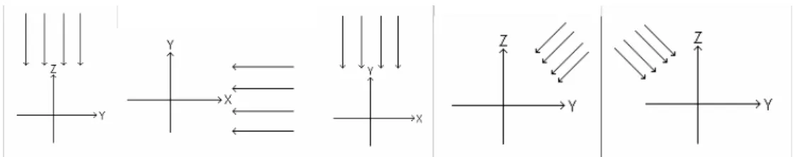
Fig. 51. Ray directions used in generating projections. Each ray direction corresponds to

a projection plane whose normal lies in the opposite direction of the corresponding ray direction.

Fig. 52. Means of performance measures obtained from 50 simulations each involving

200 points

Fig. 53. Average standard deviations of performance measures obtained from 50

simulations each involving 200 points

Fig. 54. Average performance measure displayed in logarithmic gray level. The x-axis

stands for number of projections while y-axis for number of points.

Fig. 55. Standard deviation of performance measures is displayed in logarithmic gray

(10)

(11)

Chapter 1 Introduction

1.1 Statement of the Problem

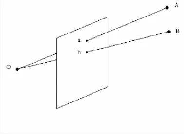
Perspective projection maps points A and B to points a and b on the plane, respectively, as can be seen in Figure 1 where O represents the focal point.

Figure 1 Perspective projection

Orthographic projection is a special case of perspective projection. When the focal point O in Figure 1 goes to infinity along the optical axis, those rays in Figure 1 become perpendicular to the image plane, thus, the projection becomes orthographic.

(12)

Orthographic projection has been used by architects and engineers for illustration purposes. More information on orthographic projection can be found in Chapter 3.

Finding shape from orthographic projections is usually studied to improve software for engineering drawings. Senda [18] reconstructs solids from three orthographic views. These views are top, side and front views. Senda uses ridgelines to construct surfaces and surfaces to construct the solid. Wang [19] studied the same problem and proposed a new method to perform reconstruction in a short time. Wang uses 2D vertices to get 3D candidate vertices, 3D candidate vertices to get 3D candidate edges. From 3D candidate edges, he gets candidate faces, and from this, a 3D solid model is constructed. The algorithm provides faster execution because he uses “boundary representation” and “constructive solid geometry” methods. Liu [20] comes up with a matrix-based approach to this problem. He represents conics in matrix form and constructs the 3D solid model using this matrix along with projection matrices.

Silhouettes provide us information about the object. It is possible to extract information about shape of an object by exploiting the silhouette information. Laurentini [12] who was inspired by Brady [16] proposed the idea of finding shape from silhouettes of an object from different viewpoints. He called the resulting shape found from silhouettes as “visual hull” of an object. In his paper [12], he implicitly claims that every object has a visual hull just like they have a convex hull. Visual hull of an object is defined as the closest approximation of an object obtained from silhouettes [12]. Volumetric intersection method is used to generate visual hull of an object using silhouettes from different viewpoints. Lines starting from the optical center of the image plane and passing from the pixels belonging to the silhouette are intersected. This method is called “volumetric intersection”.

Srinivasan [29] used volumetric intersection method for 3D reconstruction along with a contour based strategy. He assumed that each object can be represented by parallel stacked contour planes that correspond to sampling in the third dimension. He developed a data structure to represent object contours lying on stacked parallel planes. Surface intersection method applied to the multi-view binary contour images was followed by a contour intersection step to generate a 3D contour representation of objects.

(13)

Matusik [13] used visual hull concept in a real-time virtualized reality application to catch up with timing requirements. His visual hull reconstruction method is image-based rather than silhouette-based. He computed visual hull of an object that is followed by texture mapping using images taken from reference views.

Point clouds are used to express the group of locations whose values are nonzero in a 3D lattice. Point clouds are chosen to be reconstructed because some kinds of lesions appearing in some medical imaging techniques can be modeled using them. An example of such lesions is grouping of microcalcifications visualized by a mammatome apparatus (see Figure 3). Those lesions are assumed to be grouped in the tissue. Therefore, point clouds stand for opaque regions that mimic those lesions. Locations of point clouds should be obtained exactly by the reconstruction process for subsequent operation. Carr [17] uses basic trigonometry and parallax shift to locate breast lesions.

The purpose of this thesis is to reconstruct point clouds from multi-view orthographic projections. Point clouds are generated through stochastic processes. Their orthographic projections are generated from any possible viewpoint. Point correspondences between these orthographic projections could not be found correctly. For this reason, volumetric intersection method is carried out to reconstruct point clouds from multi-view orthographic projections. A performance measure is devised to assess reconstructions upon observing erroneous reconstructed points. A series of experiments are performed to investigate the effect of number of projections and number of points to reconstruction.

1.2 Motivation

At the beginning, the motivation was to devise a method that automates the localization of breast lesions. Current mammatome technology require a physician to mark the lesion locations on mammography images. Triangulation using the corresponding marks on mammography images is applied along with basic trigonometry to find the 3D locations of breast lesions in a mammatome apparatus. Breast biopsy is done using a needle following the localization of breast lesions. In this work, the desirable course of study was to devise a method that automates 3D localization of breast lesions from actual mammatome images. Lesion positions were to be extracted from the

(14)

input mammatome images using image processing techniques. Moreover, volumetric intersection method was to be applied to find candidate locations of the lesions in the desirable course of study. Proper error correction methods are to be applied to improve the presicion and accuracy of lesion locations. However, we could not followed this course of study: we were not able to receive sufficient amount of real mammatome data. We made some attempts to collaborate with research centers studying breast cancer so that they could provide us with mammatome images. The attempts failed and we chose to proceed without using real data. Indeed, there was not enough time or resources to seek further for sources of mammatome data. So, we changed the purpose of this thesis. The main purpose was redefined to be the reconstruction of 3D point clouds from their orthographic projections.

Therefore, we artificially generated data using orthographic projections of point clouds. They are generated inside a discrete 3D lattice using stochastic methods. The stochastic methods are designed in such a way that points are distributed inside a discrete 3D lattice according to a desired distribution. Point clouds may be designed to represent lesions in breast tissue. Indeed, a thorough study should have carried out to derive statistics of distribution of lesions in breast tissue so that point clouds can statistically model lesions. However, there was not enough mammatome images to derive statistics of distribution of breast lesions and a study that derives the statistical distribution of breast lesions was not encountered in the literature. For this reason, we generated point clouds such that we believe that they mimic lesions in breast tissue to the best of our judgement. Orthographic projections of point clouds are generated and these orthographic projections are used as input data to this method.

1.3 Scope and Outline of This Thesis

This thesis is about 3D reconstruction of point clouds using multi-view orthographic projections. The proposed reconstruction method is developed using the visual hull concept and the volumetric intersection method. There are six chapters in this thesis. Chapter 1 is the introduction with background information. Chapter 2 explains the

(15)

in this Chapter as well. 3D reconstruction using multi-view orthographic projections is the subject of Chapter 3. Visual hull concept is explained in Chapter 4. Results of the proposed reconstruction method as well as performance evaluation and comparison of the reconstructions are included in Chapter 5. Conclusions and future work are the subjects of Chapter 6.

(16)

Chapter 2 Point Cloud Generation Using 3D

Stochastic Methods

Let L denote the set of all locations in a finite discrete 3D lattice and let s denote a location on the lattice. The finite discrete 3D lattice has the shape of a cube for the sake of simplicity. Discrete locations inside the finite discrete lattice are elements of the set L. These locations, denoted by s∈L, are composed of three components as s=

[

x y z

]

T

where x, y, and z are integers representing the cartesian coordinate variables and T stands for transpose operator. Now, let f be the function that maps L into B whereB=

{ }

0,1 . A point is defined as a single location, s, inside the finite discrete 3D lattice such that f

( )

s =1. A point corresponds to a sample of an opaque region. It is used in the same meaning as opacity in this thesis. According to the same argument, binary 0 corresponds to transparency whereas binary 1 corresponds to opacity. Therefore, point clouds can be defined as the set PC,PC ⊆L, that is composed of s such thatf

( )

s =1. Point clouds can contain any integer number of points in the closed interval [0,N3] where N is one side-length of the cubic finite discrete 3D lattice.

Figure 2 illustrates a finite discrete 3D lattice structure. In this Chapter, point clouds are generated using a stochastic model. Before going into the details of the stochastic model, the motivation of utilizing point clouds is explained below.

Microcalcifications are tiny spots of calcium in the breast. They are a sign of harmless cancer type that can turn into harmful type in a decade. They are formed when calcium ions start to accumulate on cell membranes in breast tissue. Coordinates of microcalcifications are used in localization of such lesions for biopsy. The distribution of microcalcifications in breast tissue differs from patient to patient. The point clouds are to

(17)

mimic the opaque regions in X-ray tomography like microcalcifications. They correspond to regions whose intensity is distinguished from their neighborhoods.

Figure 2 3D discrete lattice structure

(18)

2.1 The Stochastic Process

Finite discrete 3D lattice structure has been defined and illustrated in Figure 2. Point clouds are going to be generated inside a finite discrete 3D lattice, L. The stochastic process generates point clouds in three steps: (1) choosing cluster centers according to uniform distribution, (2) determining cluster size, shape and orientation, and (3) generating texture of clusters using Gibbs sampler. A cluster is a group of points gathered around some center that is called as “cluster center”.

2.1.1 Cluster Centers

The cluster centers are initially chosen to be random vectors of three elements, namely, p=

[

a b c

]

T where {a, b, c} are uniform random variables in the interval

[

0, 1

)

and p∈L. The random vector p is scaled to lattice dimension by using a linear scale factor so that the cluster centers are distributed inside the discrete 3D lattice in a uniformly distributed fashion. The elements of p are rounded to the nearest integer after scaling operation. The cluster centers do not have to indicate opacity. Random processes are used because lesion distribution changes from patient to patient in an indeterministic way. Point clouds are generated from points clustered around the cluster centers. These points that are clustered around a cluster center are generated by stochastically processing cubes.

2.1.2 Cluster Size, Shape and Orientation

Cluster size, shape and orientation are determined by means of operations on cubes involving random variables. Before explaining the operations, cube is defined in the following. A cube is a region in a discrete 3D lattice defined by the equality, f

( )

s =1

where s=

[

x y z

]

T in the region with the constraint; x_o ≤x<x_o +d, y_o ≤y< y_o +d,

d z z

(19)

to denote the side-length of the cube, x0, y0, and z0 stand for the reference corner

coordinate variables of the cube.

Cubes with random side-lengths and random reference corner locations are generated around each cluster center. We choose d∈

{

1,2,3

}

according to probability density given in Equation (1).

(

)

{

}

    ∈ = = otherwise i if i d P 0 3 , 2 , 1 3 1 (1)

The reference corner coordinates of each cube are generated using a sequence of operations involving random variables. The purpose of these operations is to generate clusters distributed in an ellipsoidal region with correlated coordinates. A Gaussian random vector,x=

[

x₀ y₀ z₀

]

T, is generated where x₀, y₀, z₀ represent the reference corner coordinates. Those random variables representing reference corner coordinates are zero mean but their variances are random in the interval [1, 3) according to uniform distribution. Therefore, cubes are created inside arbitrary ellipsoidal regions created by varying variances in each cartesian coordinate. Later, Gaussian random vector, x, is multiplied by a rotation matrix that is illustrated in Equation (2). The purpose of this operation is to correlate coordinates of cubes and thus clusters. The rotation matrix, A, in Equation (2) is created by multiplying three rotation matrices each rotating around one of x, y and z axes with random rotation angles, α, β, γ, respectively. The corresponding equation of this matrix multiplication is also given in Equation (2). The Gaussian random variables, α, β, and γ, that denote rotation angles in radians have zero mean and unit variance. The rotation operation is performed with respect to the corresponding cluster center. Each element of the resulting random vector representing reference corner coordinates of each cube, x', is scaled by a factor proportional to a side-length of the cubic discrete 3D lattice, L. This scaling operation has no effect on the means of reference corner coordinates whereas it scales their variances by a factor proportional to the square of the smallest side-length of L. The resulting reference corner coordinates after all of the described operations are floating point numbers with respect to their

(20)

cluster center. These floating point numbers are rounded to the nearest integer so that they correspond to elements of L.

                    =           0 0 0 33 32 31 23 22 21 13 12 11 0 0 0 ' ' ' z y x r r r r r r r r r z y x           −           −           − = α α α α β β β β γ γ γ γ cos sin 0 sin cos 0 0 0 1 cos 0 sin 0 1 0 sin 0 cos 1 0 0 0 cos sin 0 sin cos A

x'=Ax where A=RZRYRX (2)

User defined number of cubes of random dimension are distributed around all those randomly obtained cluster centers. The uniform pseudo-random number generator called Mersenne Twister (MT) [1] generates all the random numbers. The Gaussian random numbers that are derived from uniformly distributed random variables are zero mean and unit variance [2].

2.1.3 Cluster Texture - Gibbs Sampler

The purpose is to process cubes described in section 2.1.2 such that the resulting point clouds resemble lesion distribution like that of microcalcifications. Gibbs sampler is employed in converting floating small cubes into point clouds whose texture simulates breast microcalcifications.

Let D denote the region containing a cube and its surrounding voxels inside the discrete 3D lattice. D consists of coordinates δ, ε, ζ where δ, ε, ζ denote integers satisfying 0 ≤ δ ≤ d+1, 0 ≤ ε ≤ d+1, 0 ≤ ζ ≤ d+1 and d is the side-length of the cube. The range of δ, ε, ζ extend from 0 to d+1 to contain the surrounding voxels where the coordinate (1, 1, 1) represent the reference corner of the cube. There is a mapping from domain D to a binary pattern as denoted by w(D). Each possible outcome of this mapping, is given as,

(

)

B

w= χ₀₀₀,χ₀₀₁,χ₀₁₀,...,χ_δεζ,... :χ_δεζ ∈

(21)

δεζ

χ represents the elements of binary number set, B, at the lattice coordinate (δ, ε, ζ). For simplicity, locations on D are represented by si and sj and formulated asD=

{ }

si .

So, w can also be defined in terms of lattice locations as w(si). Similarly, w' is also a

binary pattern defined on D as w'(D) and it can be defined in terms of lattice locations as w'(si). Let Ω represent the set of all realizations of this mapping. Thus,Ω=

{ }

w where w is

a binary pattern over the lattice denoting realizations of the mapping and d+2 is the side-length of the region D. The Gibbs distribution that is related toχ_δεζis a probability measure denoted by P on Ω as,

P w e−U( )w

Ζ = 1 )

( . (4)

In Equation (4), Z stands for the normalization constant, and U(w) is the energy function associated with each sample function [24,25].

Before expanding the energy function, cliques and clique potentials are going to be defined. Given a 3D lattice, a clique is a subset of the lattice. The set of all cliques that is denoted by Q is the same as all the subsets of the lattice. Examples of one–voxel subsets and two–voxel subsets in a 2D lattice can be seen in Figure 4. The set of all one–voxel cliques are denoted by Q1 and that of two–voxel cliques are represented by Q2. There are

( )3

2

2d+ cliques defined in a cubic 3D lattice with a side-length of d+2. Clique potential is a function defined on each such clique. Clique potentials are chosen to be position independent in our model.

Since cliques are defined on lattice locations, notation for lattice locations are going to be used in place of cliques as well. Therefore, If s₁ =

(

δ₁ ε₁ ζ₁

)

and

(

₂ ₂ ₂

)

2 = δ ε ζ

s , w

( ) { }

s₁ ∈ 0,1 and s₁∈Q₁. Similarly, w

(

s₁,s₂

) ( ) ( ) ( ) ( )

∈

{

0,0, 0,1,1,0,1,1

}

and

(

s₁,s₂

)

∈Q₂.

(22)

Figure 4 Single-voxel clique and examples of two-voxel cliques

The energy function U(w) is given by,

( )

∑

( )

∈ = Q q q w V w U (5)

where q denotes individual cliques, Q denotes the set of all cliques, and Vq represents the

clique potential in Equation (5). Illustrations about cliques can be found in [7] and in Figure 4. In this interpretation, majority of two-voxel cliques and cliques that have more than two voxels are found out to have zero clique potential after a series of calculations given in Equation (8). Only those two-voxel cliques that are in the 26-neighborhood of each other have position independent non-zero clique potentials. Therefore, the sum of clique potentials,

∑

∈Q q q w V ( ), becomes;

( )

(

)

(

∑

)

∑

≠ ∈ ∈ ∈ + = j i j i i s s Q s s j i Q s i Q q q w V w s V w s s V 2 1 , 2 1( ) ( , ) ) ( , where

(

)

(

∑

) ≠ ∈ j i j i s s Q s s s s w V 2 , 2 1

2( , ) represent the sum of two-voxel clique potentials and

( )

∑

∈ 1 ) ( 1 Q s i i s w

V represent the sum of one–voxel clique potentials. The clique potentials are defined as,

(

)

(

)

(

)

{

( ) ( )

}

  − ∈ ∈ = i j j si j i s where s s w else if a s s w V , 0,0,1,1 η 0 , 2

(

( )

)

( )

0 1 0 1 = =    = i i i s w s w if if k s w V . (6)

(23)

In Equation (6),

i

s

η represents the 26-neighborhood of si in D. 26-neighborhood is the

neighborhood scheme involving 26 voxels around the primary voxel. Rubik’s cube is used to illustrate this neighborhood scheme in Figure 5.

Figure 5 Rubik’s cube to illustrate 26-Neighborhood

Gibbs distributed probability, P(w), has been explained until now. The Gibbs sampler generates sample outcomes from this distribution. Each sample is an element of Ω. Samples are generated as a result of an iterative algorithm. Gibbs sampler starts with the initial pattern over the region D where D is defined in Subsection 2.1.3. The basic idea behind Gibbs sampler is to compare Gibbs probability (or energy) of the pattern containing all voxels inside the region D with Gibbs probability (or energy) of the modified pattern. The modification involves inversion of the binary value of a randomly picked voxel inside D. Therefore, binary value of a randomly chosen voxel of the current pattern is inverted resulting in a new pattern. And, Gibbs probability (or energy) of the current pattern is compared with that of the new pattern. At each iteration, if the new pattern yields more probable pattern (or lower energy) with respect to the Gibbs distributed probability (or energy) of the current pattern, then the new pattern is adopted as the current pattern. If, however, the new pattern has less probability, then the new pattern is adopted with a probability equal to the ratio of probability of the new pattern to the probability of the current pattern. If we denote the current pattern with w and the new pattern with w', the Gibbs sampler becomes,

(24)

( )

( ) ( ) ( ) ( ) ( ) ( ) [ ] ' , 1 ' , 1 1 1 ' ' ' ' w w r If w w e e e e Z e Z w P w P r If r y probabilit with w U w U w U w U w U w U → < → ≥ = = = = − − − − − − (7)

and this is iterated four times the number of all voxels in w for randomly selected voxels. The Gibbs sampler algorithm starts with the same pattern in each case. It is proved in [7] that the iterative algorithm yields a Gibbs sample for every starting configuration if there is enough number of iterations. It is empirically found that the iteration converges to a Gibbs sample when number of iterations is more than four times number of all voxels. This empirical derivation is supported by [7] where convergence properties of Gibbs sampler algorithm are established.

Equation (7) is further simplified by canceling all one-voxel clique potentials except for the clique potential of randomly picked voxel and by canceling all two-voxel clique potentials formulated in Equation (6) except for clique potentials composed of two neighboring voxels involving the randomly picked voxel. The cancellation is because that only a single voxel is changed when going from w to w'. All the other voxels have the same values as before. Therefore, clique potentials with respect to these unchanged voxels are the same and they yield further simplification. The cancellation and simplification is given in Equations (9) and (10). Before applying simplification and cancellation, difference of Gibbs energies of any two patterns w and w' are given as,

( )

(

)

(

)

(

∑

)

∑

(

( )

)

(

∑

)

(

)

∑

≠ ∈ ∈ ≠ ∈ ∈ ∈ ∈ − − ′ + ′ = − ′ = − j s i s Q j s i s j i Q i s i j s i s Q j s i s j i Q i s i Q q q Q q q s s w V s w V s s w V s w V w V w V w U w U 2 , 2 1 1 2 , 2 1 1 , , ' . (8)

The simplification is given in Equation (9) where the pattern w' is same as w except for the value of a single voxel, sv. Starting with Equation (8),

∑

(

( )

)

∈ ′ 1 1 Q s i i s w V can be

(25)

expanded as;

(

( )

)

(

( )

_i

)

(

( )

_v

)

Q s s s i V w s V w s s w V i i v ′ + = ′

∑

∈ ≠ 1 1 1 1 . Similarly,

(

)

(

∑

) ≠ ∈ ′ j i j i s s Q s s j i s s w V 2 , 2 , can be expanded as;

(

)

(

∑

) (

∑

)

(

)

(

∑

)

(

)

≠ ∈ ≠ ≠ ∈ ≠ ∈ ′ + = ′ j v j v v i j i j i j i j i s s Q s s j v s s s s Q s s j i s s Q s s j i s V ws s V w s s s w V 2 2 2 , 2 , 2 , 2 , , , since w' is

same as w except for the value of sv. Therefore, Equation (8) can be written as;

( )

(

)

(

)

( )

(

( )

)

( )

(

)

(

( )

)

( )

(

)

₍

₎

( ) ( )

(

)

(

( )

)

(

( )

)

(

)

(

)

(

∑

) (

∑

)

(

)

∑

≠ ∈ ≠ ≠ ∈ ≠ ≠ ∈ ≠ ≠ ∈ ≠ ≠ ∈ ∈ ≠ ∈ ∈ − − − − ′ + + ′ + = − − ′ + ′ j s v s Q j s v s j v v s i s j s i s Q j s i s j i v v s i s i j s v s Q j s v s j v v s i s j s i s Q j s i s j i v v s i s i j s i s Q j s i s j i Q i s i j s i s Q j s i s j i Q i s i s s w V s s w V s w V s w V s s w V s s w V s w V s w V s s w V s w V s s w V s w V 2 , 2 2 , 2 1 1 2 , 2 2 , 2 1 1 2 , 2 1 1 2 , 2 1 1 , , , , , , . (9)

After canceling similar terms in Equation (9) and applying the clique potentials given in Equation (6), simplification in Equation (10) is obtained.

( )

(

)

₍

₎

( )

(

( )

)

( )

(

)

( )

(

)

(

( )

)

(

)

(

)

(

∑

)

∑

≠ ∈ ≠ ∈ ≠ ∈ − ′ + − ′ = − − ′ + ′ j s v s Q j s v s j v j v v v j s v s Q j s v s j v v j s v s Q j s v s j v v s s w V s s w V s w V s w V s s w V s w V s s w V s w V 2 , 2 2 1 1 2 , 2 1 2 , 2 1 , , , ,

(

)

(

)

(

)

{

(

) ( )

}

(

)

{

(

) (

)

}

     ∈ ∈ ∈ ∈ − = − ′ v s j v s j j v j v j v j v s s where where s s w s s w else if if a a s s w V s s w V η η 0 , 1 , 1 , 0 , 1 , 1 , 0 , 0 , 0 , , 2 2 (10)

( )

(

)

(

( )

)

( )

    = = − = − ′ 0 1 1 1 v v v v s w s w if if k k s w V s w V

(26)

The algorithm is iterated four times the number of all voxels in the entire region. The resulting pattern is a Gibbs sample. The algorithm is illustrated in Figure 6 in 2D using a square in place of a cube. The initial pattern involves a 2D 3 by 3 square white region surrounded by black region as illustrated in Figure 6.a. The dimension of patterns in Figure 6 is 5 by 5. After one step of the iteration, the pattern shown in Figure 6.b is generated. After five steps, the pattern in Figure 6.e is generated. After 100 steps that is 4 times the total number of pixels, the pattern in Figure 6.f is generated.

Each cluster is processed as described and the Gibbs sample is placed inside the 3D lattice. If two overlapping clusters are encountered while placing a Gibbs sample inside the discrete 3D lattice, then values of the latter cluster overwrites the previous one. The described three step random process in subsections 2.1.1, 2.1.2 and 2.1.3 completes the generation of the point cloud.

a) b) c)

d) e) f)

Figure 6 Illustration of Gibbs sampler algorithm in 2D using a 3 by 3 square white region surrounded by black region as an initial pattern. a, b, c, d, e, f indicate evolutions with the iteration.

(27)

The algorithm can be summarized as follows:

For the designated cube, start with the pattern over the region D that contains a cube and its surrounding voxels as described in subsection 2.1.3. Although there is no obligation for the initial pattern, this pattern is chosen for easy implemention.

1. Randomly pick a voxel, sv, inside the current pattern, according to uniform

distribution. Generate a new pattern by inverting binary value of sv.

2. Compute the difference of energy functions, U(w')-U(w), as given in Equations (9) and (10).

3. Compute r that is given in Equation (7) using the result of Step 2.

4. If r ≥ 1, then adopt the new pattern as the current pattern and jump to Step 1. 5. If smaller, r < 1, then adopt the new pattern as the current pattern with probability

equal to r and jump to Step 1.

The loop is stopped when the number of iterations reaches four times the number of all voxels inside D.

(28)

Chapter 3 Reconstruction from Multi-View

Orthographic Projections

3.1 How to Generate Orthographic Projections of

Point Clouds

Point clouds are generated on a discrete 3D lattice as described in Chapter 2. After generating point clouds, their projections are going to be computed. Orthographic projection is used in this work rather than perspective projection because it models parallelized rays utilized in some medical imaging techniques.

Orthographic projection is a projection without scaling. The parallel rays incident on the projection plane are perpendicular to the plane. Orthographic projection of three points is illustrated in Figure 7.

Figure 7 Orthographic projections of three points in space

The X and Y coordinates are preserved in this projection but the depth information (Z coordinate) is lost. During orthographic projection operation, the Z value is zeroed out as can be seen from the matrix operation,

(29)

                      =           1 1 0 0 0 0 0 1 0 0 0 0 1 1 Z Y X v u λ =ΩΛ, (11)

where λ denotes the projection plane coordinates, Ω denotes the orthographic projection matrix, and Λ denotes the world coordinates of the points in homogenous coordinates.

Homogenous coordinates stem from homogenous equation of the form

0 = + +

+by cz dw

ax where a, b, c, d are scalars and x, y, z, w are homogenous coordinate variables [27]. The w variable represents the scale factor. The scale is d in the equation above. Variables a, b, and c are divided by the scale d to convert into cartesian coordinates. Therefore, homogenous [a b c d]T is equivalent to [a/d b/d c/d]T in cartesian coordinates. Homogenous coordinates are used to represent conic equations correctly in matrix and/or vector form. The difference between homogenous and cartesian coordinates is the addition of a new dimension, w. The scale in the matrix equations above is 1.

The operation of taking orthographic projection of point clouds is illustrated in Figure 8. Suppose there are three projection planes with normal vectors and points scattered in a 3D lattice as shown in Figure 8. There is a center of rotation where all normal vectors of projection planes intersect if they are not parallel. Orthographic projections of those points are taken using imaginary parallel rays retrograde to normal vectors of projection planes. The projection planes can have any possible orientation always facing the discrete 3D lattice. Imaginary parallel rays are constantly chosen to be perpendicular to the target projection plane.

(30)

Figure 8 Cross-section of projection planes and point clouds

Imaginary parallel rays pass through the 3D lattice in the opposite direction of the normal vectors of the projection planes. If they confront points during their travel, they hit the point; therefore, that is the end of their travel. Thus, binary 1s appear in the corresponding pixels of the projection planes when they encounter a point during their travel. If they do not confront anything, they reach the projection plane and a binary zero appears in the corresponding pixels of the projection planes.

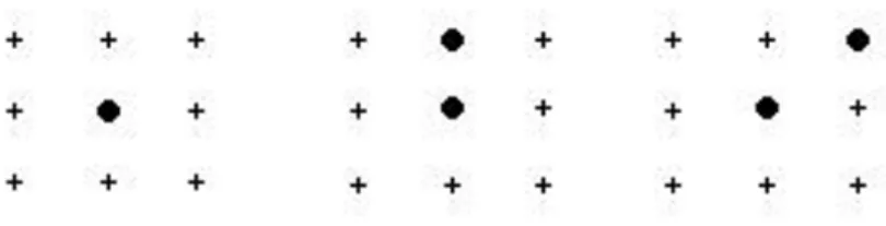
These parallel rays are designed to have any orientation. However, if continuous line model is adopted, then those continuous rays will pass through intervoxel space (see Figure 11). Detection of those lines running into points during their travel in the intervoxel space is experimented to be error-prone. For this reason, discrete line model is adopted in place of continuous line model for those parallel rays. Discrete parallel rays do not pass through intervoxel space unlike continuous ones. They pass through lattice elements along their paths. In other words, discrete rays travel in a direction by visiting nearest lattice elements as can be seen in Figure 9. In Figure 9, there are three discrete parallel rays shown by gray color on a screen composed of pixels. There are two more identical white-colored rays in between those three rays. It can be seen from Figure 9 that discrete parallel rays span the discrete 2D lattice and they do not intersect. We can generalize this conclusion and claim that discrete 3D parallel rays also span discrete 3D lattice and they do not intersect as well. Furthermore, notice that, each pixel on digital rays in Figure 9 is connected to another pixel in its 8-neighborhood. 8-neighborhood scheme is used in generating those rays so that parallel rays do not intersect with each

(31)

other whereas they do intersect if 4-neighborhood scheme is adopted. Neighborhood schemes in the plane are illustrated in Figure 10. The crosses are in the 4-neighborhood, the dots and crosses together are in the 8-neighborhood of the large point at the center.

Figure 9 Parallel discrete lines

Figure 10 Figure illustrating 4-Neighborhood and 8-Neighborhood

(32)

3.2 How to Extract Depth Information from

Orthographic Projections

There are numerous works in the literature that are dedicated to finding the lost information from projections in many ways and for various purposes [4, 5, 6, 15, 17]. In this thesis, finding the depth information of points forming point clouds inside a 3D lattice is one of the goals. One of the ways to do this is to devise search algorithms to find point correspondences between projection images. After finding point correspondences, rays emanating from those locations at different images are intersected using triangularization. The resulting intersection gives the coordinates of the reconstructed point. If point correspondences are not found correctly, then the reconstruction will not be the same as the original point clouds.

Figure 12 and 13 are orthographic projection images of point clouds taken from different viewpoints. The point clouds are generated as described in Chapter 2 and their orthographic projection is taken as explained in Chapter 3 Section a. In this Section, experiments that were carried out to find the depth information of point clouds are explained.

(33)

Figure 13 Orthographic projection of point clouds from different viewpoint

We are going to investigate projection images to devise methods for reconstruction. The white regions in Figures 12 and 13 indicate regions having a value of binary 1 and the black regions indicate regions having a value of binary 0. Those binary images are scaled for illustrative purposes. The two clusters at top left in Figure 13 are overlapped in Figure 12 as a result of projections from different viewpoints. The remaining clusters in Figure 13 have minor differences when compared to corresponding clusters in Figure 12 if observed carefully. Distinctive pixels in both figures are those that have different value than surrounding pixels. White pixels surrounded by black ones and black pixels surrounded by white pixels form those distinctive pixels.

The first approach was to apply block matching algorithm to find point correspondences. However, this algorithm did not yield satisfactory results due to merged clusters and some of the blocks could not be matched. Hierarchical block matching algorithm was applied to improve results of block matching algorithm and to allow matching algorithm to have smaller blocks when necessary. This also did not result in satisfactory results. The last experiment was to apply Lowe’s scale invariant feature transform [30] into those images. Only a small number of feature points could be extracted. The number of those feature points was not enough to calculate the angle between normal vectors of the projection planes. Although the experimented algorithms yield satisfactory results with grayscale images, they failed to function properly in binary projection images. One of the reasons is that amplitude information is not present in binary images.

(34)

If correspondences were found correctly, then rays emanating from matched points would be intersected. The coordinates of the intersection of those rays would be claimed to belong to the original point. However, when the correspondences are not found correctly, then reconstructed object will be different from the original one. Therefore, if correct point correspondences cannot be found, then algorithms involving point correspondences should be given up. An alternative method is to intersect all the rays emanating from white pixels of all projection images instead of intersecting them one at a time. It is experienced from the previous method that there will be intersection points that do not belong to the original point clouds. These points will be handled by further processing. Figures 20 and 21 illustrate intersection of rays. These rays travel in the direction of normal vectors of their planes. This method is called volumetric intersection and explained in Chapter 4. The intersection points form clouds of points called visual hull of point clouds. Visual hull is also explained in Chapter 4. Obviously, the resulting reconstruction has more points than the original point clouds. Therefore, this thesis continues with methods devised to improve reconstructions of point clouds.

(35)

Chapter 4 Visual Hull

4.1 Convex Hull

Suppose we have a set S in multi-dimensional space. S is defined to be convex if any line segment joining any two points, m∈S and n∈S, is inside the set. In Figure 14, the second set is not convex whereas the first is because the line joining m and n contains points outside the set S [8, 9, 10, 11].

Figure 14 Convex and non-convex sets

Figure 15 A line segment, a triangle and a tetrahedron

A line segment is an example of one-dimensional convex set. A triangle is the example of two-dimensional convex set with minimum number of vertices. Likewise, an example of three-dimensional convex set is a tetrahedron (Figure 15). Notice that, the points on a line segment can be computed using linear combination of its endpoints. Moreover, the points inside a triangle can be computed from the linear combination of its

(36)

vertices. Likewise, the linear combination of corners of a tetrahedron gives the points inside it. These linear combinations should be such that the coefficients must be nonnegative and they must add up to 1. This is called the convex combination [8, 9, 10, 11]. Suppose there are k points that form a convex set namely x1, x2,…, xk. Then, convex combination is formulized as:

α₁x₁+α₂x₂ +...+αkxk with αi ≥0 ∀i and α₁+α₂ +...+αk =1 (12)

Convex hull is also a convex set. Convex hull of S is the smallest convex set that contains S. In other words, it is the intersection of all convex sets containing S. All the points contained in the convex hull of S can be calculated using convex combinations of points of S. The proof is trivial.

Before going into the convex hull in a plane, I need to define the extreme points. A point in S is not an extreme point if it lies on the open line segment formed by any two points in S. Moreover, a point is not an extreme point if it lies inside the triangle formed by three points that are element of S, not on the triangle. Those points that are not one of the above are extreme points. Therefore, the convex hull of extreme points is the same as the convex hull of the point set. So, in order to find the convex hull of S, all I need to do is to find the extreme points and connect them in some order. There are numerous algorithms to compute the convex hull in plane. A few of them are “quickhull” [8, 10], “Graham scan” [8, 10, 11] and “incremental algorithm” [10, 11]. An illustration of a convex hull in a plane is given in Figure 16 where extreme points are the ones connected with lines.

(37)

Convex hull is a polyhedron in space which looks like the one given in Figure 17. Convex hull in space can be treated in the same way convex hull in plane is treated. Some of the 3D convex hull computation algorithms are extensions of 2D algorithms into 3D. Convex hull in space may be computed using the “incremental algorithm” [8, 10], “gift wrapping” [10] or the “randomized incremental algorithm” [10].

Figure 17 Convex hull of a polyhedron in space

4.2 Visual Hull

Consider the traffic signs in Figure 18.

Figure 18 Traffic signs

There is a silhouette of a man walking: a pedestrian. From this silhouette, we understand that there is a regulation related to pedestrians. Similarly, the sign with a silhouette of falling rocks tells us that rocks may fall or have fallen. Those signs with silhouettes of a bus and a bike give us useful information as well. Indeed, our brains recognize objects from the silhouette information provided. The information provided by

(38)

silhouettes is not detailed and can be deceptive as well. However, there exist situations where detail or ambiguity is not critical. The concept of visual hull emerged from the idea of using silhouette information in 3D reconstruction.

The visual hull is a 3D concept. The aim is to recognize or to recover the shape of an object. Constructing visual hull of an object requires volumetric intersection method that is explained in Chapter 4, Subsection c. Briefly, volumetric intersection method intersects cones from all the silhouettes to get the visual hull. The tops of these cones are the optical centers of the images. In this thesis, orthogonally projected images are used, therefore, cones become cylinders. Visual hull that is constructed using the volumetric intersection method with respect to proper viewpoints approximates an object. The closeness of this approximation depends on the number of silhouettes, convexity of the object and the width of the viewing region. If the object is equal to its visual hull, then the volumetric reconstruction is perfect [12]. Convex hull contains the visual hull and together they contain the object. In mathematical notation: CH(Θ_)⊇VH(Θ_)⊇Θ_whereΘ_{denotes the}

object [12]. Taking projections of an object and its visual hull with respect to same viewing regions result in equivalent silhouettes. Moreover, two objects can be distinguished from their silhouettes according to the same viewpoint if and only if their visual hulls are different [12]. Otherwise, they yield the same silhouettes from the same viewpoints.

4.3 Volumetric Intersection Method

The volumetric intersection method is applied to build the visual hull of point clouds. Let Vi denote the cylindrical volume constructed by sweeping the ith silhouette; then the

volumetric intersection method provides the visual hull, VH, built from n silhouettes

according to n _i i n V VH 1 =

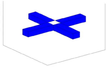
= I [13]. As n becomes infinitely large and all possible viewpoints are included, VHn converges to a shape called VH∞ of the object of interest. Figure 19 illustrates this method using two silhouettes.

There are two image planes in Figure 19 each with square silhouettes in them. Those square silhouettes are swept in the normal directions of their planes and the volume

(39)

emerged by their intersection is the visual hull. This volume is highlighted using white color in Figure 19. If the silhouettes were taken by perspective projection, then cones were to be intersected [12, 13].

The volumetric intersection algorithm developed in this thesis emanates parallel discrete lines from silhouettes in the normal direction of the projection planes. Considering those 3D lattice locations as bins, each line adds 1 to the bin as they pass through. Therefore, the intersections of all silhouettes are those bins that have a value equal to the number of silhouettes. The coordinates of those bins are gathered to construct the visual hull of point clouds.

(40)

4.4 Removal of Undesired Reconstructions

The visual hull of point clouds is not equal to the original point clouds for most cases. In order to always have perfect reconstruction; the number of projection planes has to be larger than the number of points. The reason for this is illustrated in Figures 20 and 21.

Figure 20 Reconstruction of 2 points using 2 image planes

Figure 21 Reconstruction of 2 points using 3 projection planes

Figure 20 illustrates volumetric reconstruction method using 2 image planes each consisting of 2 “white” pixels. The resulting reconstructed points are A, B, C, and D. Points A and D alone gives the same silhouettes on both projection planes. Likewise, C and B give the same silhouettes. Even A, B, C, and D all together do so. There is an ambiguity in this reconstruction. There are three candidates for original points. This ambiguity is eliminated by introducing a new projection plane as in Figure 21. Points B and C remain the only solution of this reconstruction. From the above discussion, we can conclude that total number of points should be less than the number of distinct projection

(41)

planes for perfect reconstruction from silhouettes of any arrangement of points. Although there are cases where less number of silhouettes than total number of points yield perfect reconstructions, this statement offers perfect reconstruction for majority of cases. Of course, there are exceptions to this statement. Any closed volume whose interior voxels are empty, i.e. 0, is an exception to this statement. No matter how many different projections are used, they always yield a reconstruction with occupied interior voxels.

When the total number of points exceeds the number of distinct projection planes, aliases or incorrect reconstructions are likely to occur as in Figure 20. Larger number of silhouettes than the total number of points in 3D discrete lattice has to be used to avoid this kind of error in reconstructions. However, this is not possible in reality. When total number of points gets reasonably large, it is not possible to design required number of distinct projections. Therefore, this kind of error is likely to occur in volumetric reconstruction. The approach adopted to deal with this error is to adjust number of projection planes and their orientation so that this kind of error is minimized.

Another source of undesired reconstructions is that digital lines having smaller angle between them do not intersect at a single voxel; instead they intersect over several consecutive voxels due to the discrete nature of those lines. See Figure 22 for an illustration.

(42)

Therefore, several consecutive voxels are reconstructed representing a single voxel. Projection planes whose normals have dot product close to 0 should be used in taking projections to avoid multiple voxels representing a single voxel. This is illustrated in Figure 23.

(43)

Chapter 5 Experiments, Performance Assessment

and Comparison

Simulation software is developed that takes orthographic projections of point clouds as input and generates a video file as output. The video file is created to display both original and reconstructed point clouds side by side. Original point clouds lies on left of the frame whereas reconstructed point clouds on the right. The time axis of the generated video is the same as the z axis of discrete 3D lattice. Another software is also developed to generate point clouds and their orthographic projections. This software is pipelined into the simulation software.

The reconstructed point clouds that are yielded by simulation software contain erroneous reconstructions in most of the cases. The reasons for these erroneous reconstructions are mentioned in Subsection 4.4 along with the ways to avoid them. Since those ways are unrealizable in most practical cases, a performance measure is designed to determine the best reconstruction within the limitations. The designed performance measure is chosen to be a linear combination. It is based on penalizing erroneous reconstructed points according to their types. The penalties are in the form of weights. Heavy penalty corresponds to a large weight. If a point that appears in the original data is not reconstructed, then this error is heavily penalized. This kind of error is labeled as ‘type 3’ and it is denoted by subscript 3. If multiple consecutive voxels are reconstructed for a single voxel as illustrated in Figure 22, then this kind of error is labeled as ‘type 1’ and denoted by subscript 1. Type 1 error is lightly penalized. Rest of the errors are labeled as ‘type 2’ and denoted by subscript 2. Type 2 error is moderately penalized. The proposed measure is given as: M = N₁×W₁+N₂×W₂ +N₃×W₃ where M denotes performance measure, N1 and W1 denote number and weight of type 1 error, N2 and W2 denote those of type 2 error, N3 and W3 do those of type 3 error. The weights are fixed for

3D reconstruction of point clouds using multi-view orthographic projections