Analysis of Erlang transfer lines

^ İ’i*· '^4. i» W * ^ < -r:^ y-., fi .Jf, »rJÎ f Ê ■..'·■* ,■/.} ;л Ï·'! ',* ^ '· îf , J.^ J * Л^*І '*•4 ¥ «'βί < ,- JÍ '^· и. ^ ;,Я а-і « й ’β W■j .'■. ■■.•‘· # é Ϊ ·ν<ί^ ,-ί* ;Ц А '*'''■ o ' ^_{>i ¿ t'ir'.^'İ^İ^U^} £г""3 :^‘ '£HReM3 £^LKe-n· uNîi/; : '■?■ Ϊ 'Ι i ; i чіЛГ w іГ, fO ft ΤΗΞ DSSnSH

^ s r m о?

ANALYSIS OF ERLANG TRANSFER LINES

A THESIS

SUBMITTED TO THE DEPARTMENT OF INDUSTRIAL ENGINEERING

AND THE INSTITUTE OF ENGINEERING AND SCIENCES OF BILKENT UNIVERSITY

IN PARTIAL FULFILLMENT OF THE REQUIREMENTS FOR THE DEGREE OF

MASTER OF SCIENCE

N&hal^ai·

By

Nebahat Dönrnez

Febmarv, 1997

f r.· ■■'Í r»·

Ъ 4 {;) /О

Ä О

■ ЬЬ4

11

I ( ertify that I have read this thesis and that in my opinion it is fully adequate, in scope and in quality, as a thesis for the degree of Master of Science.

Assoc . PW ; CCema^d3in?er( Principal Advisor)

I certify that I have read this thesis and that in my opinion it is fully adequate, in scope and in quality, as a thesis for the degree of Master of Science.

Profi^Halim Doğfûsöz

I certify that 1 have read this thesis and that in my opinion it is fully adequate, in scope and in quality, as a thesis for the degree of Master of Science.

.\ssoc. Prof! Erdal Erel

.\pproved for the Institute of Engineering and Sciences:

Prof. Mehmet Bg^y

ABSTR.\CT

ANALYSIS OF ERLANG TRANSFER LINES

Nebahat Dönmez

M.S. in Industrial Engineering

Supervisor: Assoc. Prof. Cernal Dinçer

Februarv, 1997

Transfer lines are widely used in the modeling and analysis of complex pro­ duction systems. The literature is mostly devoted to the analysis of transfer lines with exponential processing times. However, most of the time a part is |)rocessed through stages(phases) of exponential processing times. It is pos- sil)le to model such systems by means of processing times that are A,·—Erlang distributed. In the modeling and solution of these systems, significant dif­ ficulties arise due to the nature of the problem. In this thesis, we propose a -Markov model for transfer lines consisting of n reliable machines with A—Erlang processing times and finite buffers. The arrivals to the system is Poisson dis­ tributed. A program coded in C which is capable of solving the Markov model of a three machine transfer line is also developed. Besides the commonly used performance measures, such as utilization of the machines, mean throughput, mean WIP level, we calculate the variance of VVIP so that it is possible to construct confidence intervals.

Key words: Transfer Lines, Markov Models, Erlang Distribution, Variance

of WTP Level.

ÖZET

K-ERLANG

ZAMANLI SERİ AKIŞLI İMALAT

SİSTEMLERİNİN ANALİZİ

Nebahat Dönmez

Endüstri Mühendisliği Bölümü Yüksek Lisans

Tez Yöneticisi: Doç. Dr. Cemal Dinçer

Şubat, 1997

Seri akışlı imalat sistemleri karmaşık imalat sistemlerinin modellenınesinde yaygınca kullanılan alt modellerdendir. Bugüne kadar büyük çoğunlukla üssel işlem zamanlı makinelerden oluşan seri akışlı sistemler incelenmiştir. .Ancak, bir çok durumda işlem zamanları üssel evrelerden oluşmaktadır. Bu tür sis­ temleri A--Erlang dağılımı ile modellemek mümkündür. En genel haliyle bu tür sistemlerin modellenmesi oldukça büyük zorluklar içermektedir. Bu tez çalışmasında n tane A--Erlang işlem zamanlı makineden oluşan, seri akışlı ve sonlu ara stoklu. üssel talep geliş zamanlı bir sistemin Markov modellenmesi önerilmektedir. 3 makineden oluşan sistemin Markov model çözümü için C dilinde bir program kodlanmıştır. Ayrıca, geleneksel performans ölçütlerinden: makine kullanımları, ortalama üretim miktarı, ve ortalama ara stok seviyelerinin yanı sıra, ara stok seviyesinin varyansı da hesaplanmakta, böylelikle güven aralığı hesaplamalarının yapılması mümkün kılınmaktadır.

Anahtar sözcükler: Seri Akışlı Sistemler, Markov Modeller, Erlang Dağılımı,

Ara Stok Seviyesinin Varyansı

ACKNOWLEDGEMENT

I am mostly grateful to Associate Professor Cemal Dinçer for suggesting a research topic full of enthusiasm, and for his invaluable guidance, encourage­ ment and the enthusiasm he inspired on me during this study.

I am indebted to Professor Halim Dogrusoz and .\ssociate Professor Erdal Erel for showing keen interest to the subject m atter and accepting to read and nn iew this thesis. Their remarks and recommendations have been invaluable.

1 would like to express my deepest gratitude and thanks to my office mates. 1 am especially thankful to Bahar Yetiş Kara and .Muhittin Hakan Demir for their encouragement, suggestions, help, friendship, patience, understanding and moral support especially during my illness. I would also like to thank .Meltem Karasu Demir and Kadri \'etiş for everything.

Finally. I have to express my sincere gratitude to my family, and to all my dear friends for sharing everything.

C ontents

1 IN T R O D U C T IO N

1.1 Related Literature

1.1.1 Flow Lines with No Intermediate S torage... 3 1.1.2 Flow Lines with Finite Buffers

2 AN ALYSIS O F T R A N S F E R LIN ES

2.1 Solution Techniques

2. 1.1 Exact Solution T echniques... 9 2. 1.2 .Approximate Solution Techniques... IS

2.2 Problem Definition and Solution Procedure 20

3 E X P E R IM E N T A L R E SU LTS 28

4 C O N C L U S IO N 62

List o f Figures

1.1 Schematic diagram of a queueing process ... ^

1.2 Representation of a ¿-machine transfer line with k - 1 interme­ diate buffer storages ... .y

2.1 Coxian distribution with s p h a s e s ...

2.2 Phase-type distribution with s phases pj

2..'1 Flow line d eco m p o sitio n ...

2.4 .J-rnachine saturated k-Erlang transfer line with Poisson (A) ar­ rivals ... .y.y

2.0 Use of the Erlang for phased service... .>-j 4.1 Utilization of machines for K =2, A = l, and varying buffer sizes

and machine processing rates ...

•1.2 Expected WIP for K = 2, A=l, and varying buffer sizes and ma­ chine processing r a te s ...

i.-i \'ariance of WIP for K=2, A = l, and varying buffer sizes and

machine processing r a t e s ...

•4.4 Utilization of machines for K=4, A=l. and varying buffer sizes and machine processing rates ... 34

•3.0 Expected \\ IP for K=3, and varying buffer sizes and ma­

chine processing r a te s ...

-j-4.6 Variance of WIP for K=3, A=l, and varying buffer sizes and

machine processing r a t e s ...

LIST OF FIGURES ix

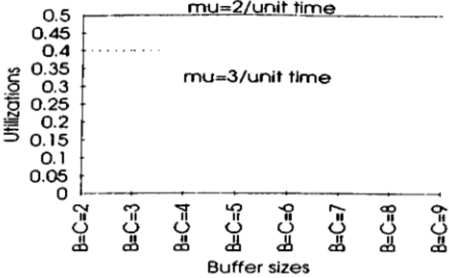
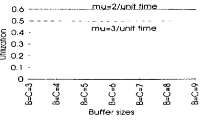
3.7 Utilization of machines for fi.xed processing rate 2/unit time, A=l, and varying buffer sizes ... З6 3.8 E.xpected VVIP for fixed processing rate 2/unit time, A=l, and

varying buffer s i z e s ... З6 3.9 Variance of VVIP for fixed processing rate 2/unit time, A=l, and

varying buffer s i z e s ... 37 3.10 Utilization of machines for K=3. A=l, ^i=2/unit time, and

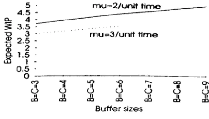
varv-ing buffer sizes ... 37 3.11 Expected WIP for K=3, A=l, //= 2/unit time, and varying buffer

s i z e s ... 33 3.12 Variance of VVIP for K=3, A=l, /i=2/unit time, and varying

buffer sizes... 33 3.13 Utilization of machines for K=3. A=l. /i=2/unit time, and vary­

ing buffer sizes ... 39 3.14 Expected VVIP for K=3, A=l, /j= 2/unit time, and varying buffer

s i z e s ... 39 3.15 V'ariance of VVIP for K=3, A=l, /i=2/unit time, and varying

buffer sizes... 49 3.16 Utilization of machines for K=3. A=l. /i=2/unit time, and

varv-ing buffer sizes ... 40 3.17 Expected VVIP for K=3, A=l. /¿=2/unit time, and varying buffer

s i z e s ... 41 3.18 Variance of VVIP for K=3, A=l. fi='2/unit time, and varying

buffer sizes... 41 3.19 Expected VVIP for K=3, A=l. /zi = 2/unit time, /<2 = 3/unit

time. /¿3 = 4/unit time, and varying buffer s i z e s ... 42 3.20 Variance of WIP for K=3, A=l. /zi = 2/unit time, /¿2 = 3/unit

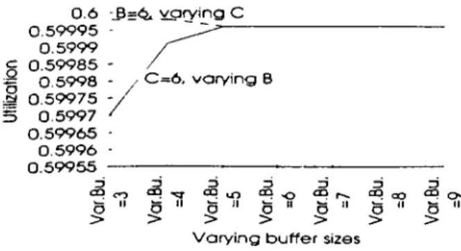
time, /¿3 = 4/unit time, and varying buffer s i z e s ... 42 3.21 Mean throughput for K=3, C = 6. A=l. and varying buffer sizes

LIST OF FIGURES

3.22 Expected VVIP for K=3, C =6, A=l, and varying buffer sizes and

machine processing r a t e s ... 3.23 Variance of WIP for K=3, C =6, A=l, and varying buffer sizes

and machine processing rates ...

43

List o f Tables

2.1 Classification of Maikov Processes...

■kl Performance measures for A'=2. f.i = 2 /unit time, varving but identical buffer sizes ... ■{.2 Performance measures for A'= 2. /i = 3 /unit time, varying but

identical buffer sizes ... ^ 3.3 Performance measures for A'=3. /i = 2 /unit time, varying but

identical buffer sizes ... 3.1 rVrformance measures for A'=3. ¡.i = 3 /unit time, varying but

identical buffer sizes ... 3.·') Performance measures for A'=3. ¡.i = 2 /unit time, varying buffer

s i z e s ... 47 3.6 Performance measures for A'=3, A = 10/unit time./i = 2 /unit

time, varying buffer s iz e s ... 3.7 Performance measures for A'=3. // = 2 /unit time, varying buffer

s i z e s ... 49 3.8 Performance measures for A'=3. ¡.i = 2 /unit time, varying buffer

s i z e s ... 49

3.9 Performance measures for A'=3. = 2 /unit time, varying buffer

s i z e s ... .50

3.10 Performance measures for A'=3, f.i = 2 /unit time, varying buffer s i z e s ... oO

3. 11 Performance measures for A'=3, = 2 /un it time, varying buffer

s i z e s ... oO 3.12 Performance measures for A'=3, A = 1 /unit time,/¿i < /.¿2 < /¿3.

and varying buffer sizes... ol

3.13 Performance measures for A'=3, A = 1 /unit time, /¿i > > ^¿3, and varying buffer sizes... .52 3.14 Performance measures for A'=3. A = 1 /unit time, /¿i > ¡.12 < //3,

and varying buffer sizes... .33 3.I0 Performance measures for A' = 3, A = 1 /unit time, /¿i < fi2 >

/Сз . and varying buffer s i z e s ... .54 3.16 Performance measures for A'=2. /i = 2 /unit time, varying buffer

s i z e s ... ~)o .3.17 Performance measures for A’=2. /г = 2 / unit time, varying buffer

s i z e s ... 06

3.18 Performance measures for A'=4. /i = 2 /unit time, varying buffer

s i z e s ... .)6 •3.19 Performance measures for A’=4. fi = 3 /unit time, varying buffer

s iz e ... oT 3.20 Performance measures for A'=2/unit time. A = l/unit time, and

varying processing rates ... .>8 3.21 Performance measures for A’=3/unit time, A=l/unit tinte. and

varying processing rates ... .59 3.22 Performance measures for A'=4/unit time. A =l/unit time, and

varying processing rates ... 60 3.23 Performance measures for A'=4/unit time, A =l/unit time, and

Chapter 1

IN T R O D U C T IO N

In this thesis, vve investigate the performance measures of a tandem queueing system with three machines with k-stage Erlang processing times, and two finite storage buffers.

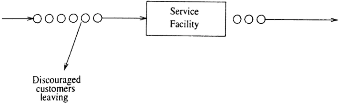
.A. queueing system can be described as customers arriving for service, waiting for service if it is not immediately available and leaving the system after being served. Such a basic system can be schematically depicted as in f igure l.l.

- ^

000,0

0

-Discouraged

customers

leaving

Figure 1.1: Schematic diagram of a queueing process

A transfer line is a manufacturing system with a very special structure.

It consists of material, work stations, and storage areas. Actually, it is a linear network of service stations/machines (A/i, 1M2___ A/jt) separated by buffer stor­ ages (Bi, B2. .., Bk-i)· Material flows from outside the system to machine Mi ,

then to buffer storage B \, then to M2, and so forth until it reaches machine Mk

after which it leaves the system. Material visits each work station and storage area exactly once in a fixed sequence. Figure 1.2. depicts a transfer line. The sc|uares represent machines and the triangles represent buffers.

In the language of queueing theory a transfer line can be represented as a finite buffer tandem queueing system. In that case, machines are called •serrers, storage areas are called buffers, and discrete parts are called customers or jobs.

CHAPTER 1. INTRODUCTION 2

M , M- M,

Figure 1.2: Representation of a /.--machine transfer line with k — 1 intermediate buffer storages

1.1

Related Literature

Transfer fines are studied due to their economic importance. They are used in high volume manufacturing, particularly in automobile production. In automobile production, the capital costs range from S 100.000 to ^30.000.000. Furthermore, transfer lines represent the simplest form of interactions of man­ ufacturing stages, and their decoupling by means of buffers. The study of coupling and decoupling leads to application to more complex systems.

The earliest theoretical papers were published in 1950's in Russia. \ ladzievskii [49] is the first author to use probability theory to explain the behaviour of automatic transfer lines. There are three major problems in the de’sign and operation of production lines. These are the number of stages in the line, the location of buffers and the buffer sizes. Tools for the solution of these problems did not appear until the 19S0’s. Buzacott and Hanifin [9] describe physical and mechanical issues , such as the transfer mechanism, shunt versus series banks which determine the movement of material according to LIFO or FIFO, and the design of the line in order to reduce the cycle time. Smunt and

Perkins [46] focus on asynchronous flow lines with reliable machines. They are interested in line design, the problem of sizing and locating the buffers, and task allocations to work stations.

Transfer line systems can be clcissified into three categories. Syn­ chronous systems are the systems in which operation times of the machines are assumed to be deterministic and equal, and when machines are not under repair, they start and stop at the same instant. In asynchronous systems, ma­ chines are not constrained to start or stop their operations at the same instant.

synchronous systems are usually modeled with random operation times. Fi­ nally. continuous models treat material flow as continuous rather than discrete. The literature reviewed here and this study considers cisynchronous transfer lines.

CHAPTER 1. INTRODUCTION 3

1.1.1

Flow Lines w ith N o In term ed ia te Storage

For transfer lines with reliable machines, Rao [43] and Lau [29] pro­ vide e.x'plicit expressions for calculating the production rate for exponentially. Erlang, uniform, and normally distributed processing times.

Hunt [25]. Hillier and Boling [23], Hildebrand [22] investigated the threee machine transfer lines with no buffer. Muth [33], Rao [44, 45] obtained numerical solutions for specific distributions of the processing times. Muth and AlkalF [35] provided a unifying solution under the assumptions that machines ,\/i and Mi have special phase-type distributions and machine M2 has a Laplace t ransformable distribution.

Papadopoulos and O’Kelly [38] develop an exact procedure for the analysis of a transfer line with reliable machines where the processing times are exponentially distributed. The exact algorithm gives the marginal probability distribution of the number of units in each machine, mean queue length, and the throughput. Papadopoulos [37] also provides an algorithm for the efficient

computation of the throughput rate of multistation reliable production lines with no intermediate buffers by extending the work of Muth [33].

For the Ccise of transfer lines with no intermediate buffer and unreli­ able machines, Buzacott [7] obtained a formula for the production rate under deterministic processing times and general up and downtime distributions as­ sumptions. Commault and Dallery [12] propose a method for calculating the production rate when uptimes are exponentially distributed.

1.1.2

Flow L ines w ith F in ite Buffers

CHAPTER 1. INTRODUCTION 4

For transfer lines with reliable machines, Rao [44] analyzed two-machine transfer lines with exponential and general processing time distributions. When the processing time of the first machine is exponentially distributed and the distribution of the processing time of the second machine is general, the line is equivalent to an M / G / i / L queue. This equiv^alance also holds for the case of a two-machine transfer line with general and exponential processing time distri­ butions for the first and second machine, respectively [14]. If the distribution of the processing times of both machines is exponential, the analysis of the line reduces to that of an M / M / l / L queue which has a simple geometric form.

For a two-machine flow line with reliable machines where the process­ ing time distribution of each machine follows a continuous phase-type distribu­ tion. the behaviour is characterized by a discrete state, continuous time Markov |)iocess.

.\ltiok and Ranjan [2], Buzacott and Kostelski [10]. Gun and Makowski [20] analvzed such systems using recursive and matrix geometric techniques which will be discussed later in Chapter 2.

Buzacott [8] analyzes a two-station model with identical unreliable machines and a finite buffer. He assumes that operation times and repair

CHAPTER 1. INTRODUCTION

times are exponentially distributed whereas the probability of failure during each operation is constant. He provides an e.xact solution of the model using r-transforms and demonstrates that production rate is a saturating function of storage space.

Gershwin and Berman [16] study the same model except that they represent failure by an exponential distribution in time rather than a geometric distribution in the number of parts produced.

Berman [4] generalizes the work of Gershwin and Berman [16] by al­ lowing Erlang distributed processing times.

Berg, Posner, and Zhao [3] investigate the effect of machine break­ downs on service and inventory levels and obtain the stationary distribution of the inventory process for different assumptions.

Di Mascolo, Frein, and Dallery [31] develop a general purpose an­ alytical method for performance evaluation of multistage kanban controlled production system. Their approximation method can be extended to complex manufacturing systems with different assumptions.

Besides studies on computing the commonly used performance mea­ sures of transfer lines, recently much work is devoted to the optimal location and sizing of buffer inventories. Jensen, Pakath. and Wilson [26] develop a dvnamic programming model and an efficient solution procedure to solve this problem. Lau [28] studies how an unpaced transfer line's utilization is affected b\· different patterns of allocating processing time variances among the sta­ tions. He shows that the results in the literature on variance allocation are ambiguous and often contradictory. He provides extensive results to demon­ strate three desirable variance allocation characteristics he identifies: bowl; which indicates that the interior stations should be allocated less work than the end stations, symmetry, and spike; which suggests that the only variability can be concentrated into only one station and all the other stations have zero variability. Later, Pike and Martin [41] show that bowl phenomenon exists and determine optimal bowl configurations. Park [39] provides a two-phase

CHAPTER 1. INTRODUCTION

lieuiistic algorithm for determining bulFer sizes of production lines.

For the e.xact analysis of transfer lines with more than two machines, the literature is sparse. For cisynchronous lines, Gershwin and Schick [17] ex­ tended their analytic solution of two-machine, finite buffer model with the assumptions that all machines are unreliable and they all have equal and con­ stant service times.

.Although exact solutions of two-rnachine transfer lines are avilable for a wide range of models, the work done up to now indicates that it seems hope­ less to expect to obtain exact solutions of transfer lines with more machines except for some limited cases of three-machine transfer lines even when more [)owerful computers become available. Therefore, the use of approximate solu­ tions are necessary to study longer lines.

Most approximate methods rely on decomposition where the idea is to partition the original system into a set of smaller subsystems which are eeisier to analvze. Decomposition methods will be presented in Chapter 2.

.Altiok [1]. Hillier and Boling [23], Perros and Altiok [40], Pollock. Birge and .\lden [42]. and Takahashi. Miyahara and Hasegawa [48] analyze flow lines with exponential processing times. In all these papers the subsystems are finite single server queues with lost arrivals and exponential processing times. Consequently, they are equivalent to a two-machine line decomposition with exponential characterization of the upstream machines.

Pollock. Birge and .Alden [42], and Takahashi. .Miyahara and Hasegawa [48] also consider an exponential characterization of the downstream machine.

Perros and .Altiok [40] analyze transfer lines using decomposition where the downstream machines are characterized by phase-type distributions. Later, .\ltiok [1] extended this method to the case of transfer lines with phase-type processing time distributions.

Altiok and Ranjan [2],and Gun and Makowski [21] study decomposi­ tion methods for transfer lines where both the upstream and the downstream

CHAPTER 1. INTRODUCTION

macliines of each decomposed line is characterized by phase-type distributions. Besides these, several authors derived simple approximation formulas for estimating the production rate of a flow line with reliable machines in which all stations are identical. Knott [27] provides an approximation formula for the case of two-machine flow lines with identical Erlang distribution. Muth [34] obtained a formula in the case of flow lines with any number of machines but no intermediate storage. Later, Blumenfeld [5] extends M uth’s formula to flow lines with intermediate buffers.

Decomposition methods for flow lines with unreliable machines and reliable machines are based on the similar principles.

Gershwin [15] developed a decomposition method for synchronous trans­ fer lines. .Afterwards, Dallery, David and Xie [13] developed an algorithm, called the DDX algorithm^ for Gershwin's decomposition technique.

For asynchronous transfer lines, Choong and Gershwin [11] extended Gershwin's decomposition technique for lines in which all machines could have different speeds, failure rates, and repair rates and all the distributions of processing times, uptimes and downtimes are assumed to be exponential.

Glcissey and Hong [18] extend the work of Gershwin [15] and develop a decomposition method for an unreliable n —stage transfer line with (n — 1) interstage storage buffers. Their method is beised on the examination of the

n —stage line and the decomposed lines, and the relationship between the failure

and repair rates of the individual stages and the aggregate stages, they show that their method performs better.

Springer [47] proposes a decomposition method for approximating the throughput rate and the WIP level of finite-buffered exponential queues in se­ ries. The approximation decomposes the network into individual finite-buffered ciueues which are linked together through a set of nonlinear equations.

All the literature review up to here concentrated on the methods to analyze the steady-state average production rates and steady-state average

CHAPTER 1. INTRODUCTION

l)uffer levels of transfer lines. Yet, the variance of the throughput and of the buffer levels during a time period is also important.

This issue hcis been neglected so far. Only a few papers deal with the calculation of the variance of the behaviour of a transfer line over a limited tim e period. Miltenburg [.32], and Lavenberg [.30] treat two-machine transfer lines. They obtained results that are difficult to use and extend.

Variability issue is very important because of the fact that the standard

deviation of production can be high. This variability is an inherent character­

istic of production systems. Prediction of this variability is cis important as the prediction of the mean since if both the mean and the variance are calculated, t hen an interval estimate for the actual throughput and the buffer levels during a period of time can be calculated.

Basically, this is the motivation for the work done in this thesis. Fur­ thermore. as the literature review emphasizes, there are few and limited a t­ tem pts to analyze the exact analytic solution techniques of transfer lines with more than two machines and finite buffers. Second chapter is devoted to the analvsis and solution techniques of transfer lines with different characteristics. In the third chapter experimental results are discussed. Finally, last chapter covers the conclusion and future research.

Chapter 2

A N A L Y SIS OF T R A N S F E R

LINES

2.1

Solution Techniques

2.1.1

E x a ct S o lu tio n T ech n iq u es

Exact analytic solutions are important because they are better than simulations or approximations when the models constructed fit real systems closely and they provide useful ciualitative insight into the behaviour of the sy stems. Furthermore, they are the vital parts of the decomposition and ag­ gregation methods that are described later in this chapter.

.Most of the results pertaining to the exact analysis of the transfer line models are based on Markovian analysis. In order to be able to analyze the beha\'iour of the transfer line by a Markov process, the distributions have to be of special form, such as exponential or, more generally, continuous phase- type distributions in the case of continuous time models; geometric or.niore precisely discrete phase-type distributions in the case of discrete time models. .\e\ertheless, there are some exceptions most often encountered in transfer

CHAPTER 2. ANALYSIS OF TRANSFER LINES 10

lines with no intermediate storage [14].

In order to be able to fully understand the discussion related to Markov processes, we are providing some information about the definitions and classi­ fications.

A stochastic process is the mathematical abstraction of an empirical

process governed by probabilistic laws. A stochcistic process can be best defined as a set of random variables, { X{ t ) , t 6 T }, defined over some index set or I)arameter space T. X{t ) represents the state of the process at time t and T is sometimes also called the time range of the process. The process is classified as a discrete-parameter or continuous-parameter process as follows:

(i.) If r is a countable secjuerice, for e.xample,

T = { 0 ,+ l,+ 2 .···}

or

T = {0. 1, 2....} .

then the stochastic process { X( t ) , t € T } is said to be a discrete-parameter process defined on the index set T;

(ii.) If T is an interval or an algebraic combination of intervals, for example,

T = {t : —oc < t < -|-oo}

or

T — {i : 0 < i <C -|-oo}.

then the stochastic process { X{ t ) , t G T ) is called a continuous-parameter [)iocess defined on the index set T.

A discrete-parameter stochastic process { X{t),t = 0 , 1, 2 . . . . } or a

CHAPTER 2. ANALYSIS OF TRANSFER LINES ₁₁

process if, for any set of n time points ti < < ■ · · < in the index set or time range of the process, the conditional distribution of -Y(<„) . given the values of -V(/i)..Y(i2).A"(i3),...,.V (< „_,) , depends only on .Y(i„_i), the immediately preceding value; for any real numbers Ji. j:2___

Pr { .Y(<„) < Xn I .Y(<i) = Xu ■. = x„_, } = Pr { X{tn) < Xn I A'(i„_i) = X„_i }

Markov processes are clcissified according to the nature of the index set of the process and the nature of the state space of the process.

A real number x is said to be a state of a stochastic process { X{t), t G T } if there is a time point t in T such that the P{x — h < ,Y(i) < x + /i} is

positive for every h > 0 . The state space is composed of the set of all possible states. If the state space is discrete, the Markov process is generally called a

Markov chain . Table 2.1. summarizes our classification scheme for Markov

processes.

Continuous time Markov processes are naturally obtained when all the distributions in the original model are exponential distributions due to the famous lack-of-mernory property oi the exponential distribution. Hence, exponential distribution has been widely used in the literature. Yet. it is not always an appropriate candidate for representing actual distributions of real life systems especially when the distributions encountered in real systems have coefficients of variation far from one which is the coefficient of variation for exponential distribution. In order to overcome this difficulty, non-exponential distributions are represented as a mixture of exponential distributions.

The simplest distribution of this form is the Erlang distribution. A

Hypo-Exponential distribution of order k consists of a series of k exponen­

tial distributions with rates pi, p2· ■ ■ ■ · Pk- Special case of Hypo-Exponential

distribution is called A:—Erlang distribution which consists of k exponential distributions with common rate pi = p2 = ■ ■ ■ = pk = p. The random vari­

able associated with the Erlang distribution is the sum of k independent and identical exponential random variables.

CHAPTER 2. ANALYSIS OF TRANSFER LINES 12

Type of Parameter

State Space Discrete Continuous

Discrete Discrete-parameter Continuous-parameter

Markov chain Markov chain

Continuous Discrete-parameter Continuous-parameter

Markov process Markov process

Table 2.1: Classification of Markov Processes

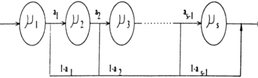
Another distribution used in the modeling of the stocheistic systems is the Coxian distribution. The Coxian distribution is more general than the Hypo-Exponential distribution since it also allows branching probabilities as shown in figure 2. 1.

Figure 2.1: Coxian distribution with s phases

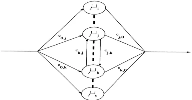
The most general form of distributions that are mixtures of exponential distributions is phase-type distribution . .\ continuous phase-type distribution with ■>' phases(stages) is represented in Figure 2.2.

If we want to give a physical interpretation of this distribution in terms of an overall task that consists of a set of s exponential subtasks. The processing time of subtask j is exponentially distributed with rate pj.

The first subtask to be completed is subtask j with probability co.j. Fpon completion of subtask j , either subtask k is performed, with probability Cj.t . or the overall task is completed, with probability Cj,o· The branching and t ransition probabilities satisfy cq.i H— - + 00.5 = 1. and cyi-f-· · · + cy, d-cyo = 1· Phase-type distributions give rise to Markovian processes by extending the original state space to incorporate the detailed information of which stage each distribution is currently in. The increcise in the size of the state space

CHAPTER 2. ANALYSIS OF TRANSFER LINES ₁₃

Figure 2.2: Phase-type distribution with s phases

is the price to pay to handle more realistic models having non-exponential distributions.

Similarly, discrete phase-type distributions can be defined. In that ca.se. the geometric distribution plays the same role as the exponential distri­ bution of continuous case.

D efinition: A probability distribution F( ) on [0, oc) is a distribution

of phase type (PH distribution) if and only if it is the distribution of the time

until absorption in a finite Markov process having the states -f 1}

with infinitesimal generator

Q =

>p rpo

0 0

where the non-singular rn x m matrix T satisfies T,, < 0, fo r I < i <

ni, and Tij > 0, fo r i j. Moreover, Te-f-T® = 0 , and the initial probability

vector of Q is given by (« ,0 ^+1) with ae-|-Q,„+i = 1 and states l , . . . , m are all transient, so that absorption into the state m -|-1 , from any initial state, is certain. The pair ( a ,T ) is called a representation of F{·).

CHAPTER 2. ANALYSIS OF TRANSFER LINES 14

The generalized Erlang distribution of order k with parameters A j,. . . , Ayt has the representation a = ( 1, 0, . . . , 0) and

T =

—Ai Ai

—A2 A2

—Xk-i Ajt_i

-A*

Discrete PH-distributions are defined by considering an rn + 1 state Markov chain P of the form

'P P'0 P =

0 1

where T is a substochastic matrix, such that I — T is nonsingular. The initial I)iobability vector is ( « ,0 ^+1)· The probability density {p^} of phase type is given by

Pq — ^m + l '

Pfc = a T ^-iT « , for k > 1.

In the analysis of two-machine flow lines with reliable machines having continuous phase-type distribution, any numerical technique for discrete space Markov processes can in principle be used. However, it is important to recog­ nize that the Markov process has a very special structure and one must take advantage of it. Let PHi refer to the phase-type distribution of machine 4/, for i = 1.2, and let .s, be the number of phases of PHi. We can characterize the behaviour of such a system by a discrete state, continuous time Markov chain and then analyze this system to calculate the steady-state probabilities of the Markov chain and derive all the performance measures.

The state of the Markov process can be expressed cis (n ,71,^2), where

CHAPTER 2. ANALYSIS OF TRANSFER LINES 15

phase of service of machine A/,, i = 1,2. n can take on integer values from 0 fo N. ji can take on integer values from 0 to Si, where j i — 0 represents the

case of blocking of machine Mi. Similarly, /2 can take on integer values from 0 to .S2, but in that case j>2 = 0 represents starvation of machine M2.

If the state space is partitioned according to the values of n, and p denotes the steady-state probability vector and p„ denotes the portion of that vector that corresponds to a buffer content of n, we can write

P = Pi

P.v J

Note that pn, n = 1. . . . , A — 1 , is of size .Si.S2 while po and p\· are of size •si and .'>2 respectively.

Let Q denote the infinitesimal generator of the Markov chain. The steady-state probability vector p of the Markov chain is the solution of the e(|uation

QTp = 0.

In addition, p also satisfies the normalization equation

l ^ p = 1.

Matrix is a block tridiagonal matrix with the following special

CHAPTER 2. ANALYSIS OF TRANSFER LINES 16 Bo Ao 0 • 0 Co B A 0 . 0

c

c

where ,4, B, C are square matrices of size (5iS2, 5152) : Bq and B ^ are square matrices of size (si, Si) and (¿2, -52): ^ 0, Cq, A y , and Cy are of size (5iS2. ). (.s,. S1.S2). {s-2, S1S2), {siS2, S2) respectively.

has this special structure because the Markov chain associated with a two-machine transfer line is a generalized birth-death process. Transitions occur only between states that are neigbours of each other with respect to the value of n . That is, the only possible transitions from a state i n . j1. j2) are to

state ( n . j [ , j2) such that n = n, n — 1, n -f 1. Moreover, transition rates are

independent of n , for 1 < n < N — 1. Because of the special block tridiagonal

structure of . ecpiation Q ^p = 0 can be decomposed into the following set of equations, which we call transition equations,

^oPo + '"foPi = 0.

T'oPo + B p i -|- /4p2 = 0.

f^'oPn-i + Bpn + -4p„4.i = 0. 1 < n < ;V — 1. Cp.v_2 + B p y - i -t- /4,\-p.v = 0,

C.vp.v-l + B y p y = 0.

The special structure of the matri.x led to two solution techniques

that make use of this special structure. These are the recursive technique and the matrix geometric technique.

For matrix geometric technique the reader is referred to Neuts [36]. The principle of the matrix geometric solution can be briefly described as

CHAPTER 2. ANALYSIS OF TRANSFER LINES 17

follows. The first step is to show that the set of transition equations can be transformed into an equation of the form

Npn + A /p„-i = 0,

where the matrices N and M are of size(siS2, S1S2) and N is invertible. If we

define a matrix R as R = —N ~^M , we have

Pn = Rpn-i^ I < n < N.

For the boundary states, if we also define matrices 5 cuid U such that = ip o and p.v = t^p,v-i- Po can be determined by solving an equation of the form Zpo = X which is obtained from the basic set of transition equations. Then, the remaining probabilities can be obtained. For more details, see Gun [19] and Gun and Makowski [20].

The recursive technique can be applied to Markov processes that sat­ isfy the condition that there exists a subset of states, boundary states, such that the probabilities of all other states can be obtained recursively from the prob­ abilities of the boundary states. The recursive technique can be implemented using the following algorithm [10].

(1) Reduction step-determine .M boundaries and derive a recursive scheme, to calculate all other state probabilities from the boundary state prob- abilities. Then, express all state probabilities as linear combinations of the i)oundary values. In order to find the coefficient of a particular boundary value in the linear expression, set that boundary value to 1 and all other boundary values to 0, and then follow through the recursive scheme. This is done M times, corresponding to the M boundaries. There will be M equations not used in the calculation of the state probabilities in terms of the boundary val­ ues. M — I of these equations together with the normalizing equation give, after substituting expressions in terms of boundary state probabilities for non­ boundary probabilities. A/ equations for the M boundary state probabilities.

(2) Solution step -determine the A/ boundary state probabilities by solving the set of A/ equations.

(3) Evaluation step -from the recursive scheme, determine the re­ maining state probabilities. Key to the use of this recursive algorithm is the

CHAPTER 2. ANALYSIS OF TRANSFER LINES 18

determination of how many boundaries to use and which specific states to be chosen as the boundary states.

2 .1 .2

A p p ro x im a te S olution T ech n iq u es

Most approximate methods are based on decomposition. Each decom­ position method involves three steps. First step is the characterization of the subsystems, then a set of equations is derived to determine the unknown pa­ rameters of each subsystem. Finally, an algorithm is developed to solve these equations.

The aim of the first step is to define how the original line is decomposed into subsystems and to characterize each subsystem. The subsystems must liave exact solutions. The second step aims to establish relationships between quantities pertaining to different subsystems so as to derive the parameters of each subsystem from the parameters and performance measures of other subsystems.

Most decomposition methods in the literature decompose a A —machine flow line into a set of A — I subsystems where each subsystem is associated with a buffer of the original line. In some methods, the subsystem is a two-machine line while in others it consists of a single server queue with a finite buffer. Since the subsystems are always simpler than the whole line, they cannot ex­ hibit the same behaviour. Moreover, some of the equations used to determine the parameters may be approximate, even within their assumptions. Thus, de­ composition methods are approximations. For the principles of decomposition methods for flow lines with reliable machines, the reader is referred to Hillier and Boling [2.3].

The decomposition approach decomposes the original A^—machine line into a set of K — 1 two-machine lines. Each two-machine line is associated with a buffer of the original line. Let L denote the original line and A(i, i -f-1) denote

CHAPTER 2. ANALYSIS OF TRANSFER LINES 19

the two-machine line cissociated with buffer Let subscripts u and d refer

to objects and parameters of the upstream and downstream machines. Machine

Mu{i. i + 1) is the upstream machine, and f+ l) is the downstream machine of line L{i, i A 1). The decomposition approach is depicted in Figure 2.3.

1 ,2 ) cIC 1 , 2 )

d C 2 , 3 )

^uC3,4.) cl(3,^)

Figure 2.3: Flow line decomposition

The basic idea in decomposition is the definition of upstream and downstream machines for each two-machine line L{i.i + 1) such that the be­ haviour of material through its buffer is close to the behaviour of material in

buffer in line L.

L’pstream and downstream machines of each two-machine line sum­ marize the effects of the entire up and downstream portions of the line, respec-

tivelv. on the buffer. For example, machine + 1) represents the portion

of the line L upstream of buffer that is, machine .\/t to machine

Likewise, machine Md{L <· + f) represents the portion of line L downstream of

buffer that is. machine A/,+i to machine Mk- In the literature, these

machines are usually called equivalent machines, pseudo-machines, or virtual

CHAPTER 2. ANALYSIS OF TRANSFER LINES 20

Furthermore, there are alternative decomposition methods which de­ compose a A'—machine line into a set of A' — 2 three-machine lines. This approach may result in more accurate results. Nevertheless, it requires repet­ itive solutions of three-machine subsystems which are too complex to solve in general as discussed before.

2.2

Problem Definition and Solution Proce­

dure

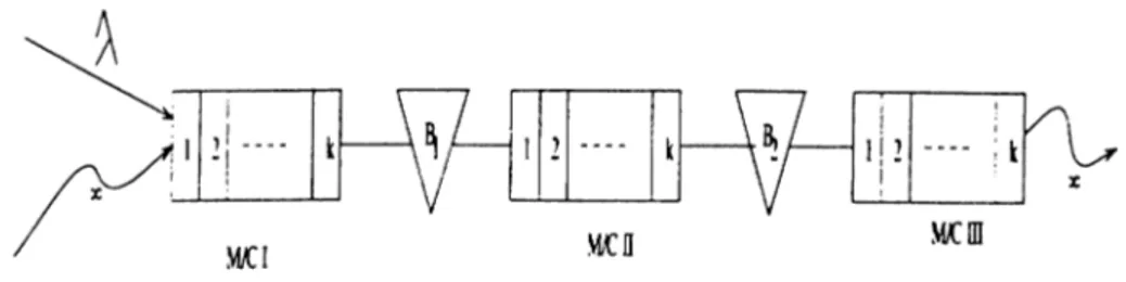
We investigate the behaviour of a transfer line with three machines and two finite buffers. Since, the machines are assumed to be reliable, the only source of randomness in the system is the random machine processing times which are assumed ^’-stag e Erlang distributed.

There are mainly four factors to be considered in choosing a distri- biitiou function. These are, factor 1, its ease of mathematical manipulation; factor 2. its ease of fitting, that is, of determining its parameters from standard

sum m ary statistics (such as mean, variance, range, etc.) of empirical data: fac­ tor 3. its resemblance to empirical distribution from actual data; and factor 4, its consistency with the '"principle of entropy maximization " .

Regarding the last factor, information theory recommends that, for a given set of statistical conditions, a distribution function that maximizes the entropy' should be adopted, subjected to the satisfaction of the given conditions. .A non-technical interpretation of entropy maximization is that the selected distribution function fully reflect the information given on the random \ariable but should not impose on it any additional assumptions.

Exponential distribution scores very well on factors 1, 2 and 4. Re­ garding factor 4, if only the mean of a non-negative random variable is known, the exponential distribution maximizes the entropy.

CHAPTER 2. ANALYSIS OF TRANSFER LINES ₂₁

The Erlang distribution is often used to represent processing times in unpaced line models since it can assume a wide range of different skewness and; therefore, be suitable for fitting real-life empirical distributions of pro­ cessing times [29]. Moreover, since the sum of k independently and identically distributed e.xponential random variables with mean l/kfi yields a it—Erlang distribution w'ith parameter /x. Erlang allows us to describe queueing models where the service may be a series of identical phcises. Hence, the most impor­ tant reason w'hy the Erlang distribution is useful in queueing analyses is its relation to the exponential distribution which is the only continuous distribu­ tion with Markovian property.

The underlying assumptions of our model are as follows. Considering the material, it consists of discrete parts and there is only a single kind of material in the system. Each piece of material visits the machines and buffers in exactly the same sequence.

The machines are not constrained to start or stop their operations at the same instant: therefore, it is an asynchronous transfer line. Machine processing times are A·—stage Erlang distributed and the time between part arrivals to the system is exponentially distributed with parameter A.

.Some models of flow lines have machines that can fail. When a fail­ ure occurs, machine cannot process any material, so the buffer upstream can­ not lose material and the buffer downstream cannot gain material. Systems in which machines cannot fail are called Flow Lines with Reliable Machines I FLR.M)'s. Our research assumes that the system is FLR.M’s.

VV henever machine A/, processes material, it reduces the le\el of buffer

and it increases the level of buffer On the other hand, when

machine A/, takes an especially long time to process a part, and its neighbour

machines work normally, the level of buffer increases and the level of

buffer decre<ises.

If this situation persists, buffer may become full or buffer

CHAPTER 2. ANALYSIS OF TRANSFER LINES 99

able to operate; either machine A/,+i is starved or machine A/,_i is blocked. In real life systems, it is possible that raw material is absent, or the means of removal of finished goods fail. We asume that the calling population is infinite and the last machine is never blocked.

Considering the operating policy, in our system, machines are not al­ lowed to be idle if they can be operated. That is, whenever a machine is neither blocked nor starved, it is used for an operation Buzacott...[30]...(1982) demon­ strates that this is the optimal operating policy for a two-machine line when the performance measure is the system production rate.

Quality is not treated in the model presented here. All parts are assumed perfect. There is no inspection procedure, no rework, and no rejects. Furthermore, the material in the storage buffers is assumed to be nonperishable.

The transfer line system we investigate is depicted in Figure 2.4. where DC S indicate that the system is saturated.

Figure 2.4: 3-machine saturated k-Erlang transfer line with Poisson (A) arrivals This system is modeled as a discrete state space continuous time -Markov chain.

Markov chain models of transfer lines are difficult to treat due to their large state spaces and their indecomposability. When the system is modeled as a discrete state Markov chain, the number of distinct states is the product of the number of different machine states, and the number of distinct buffer levels.

Many models of queueing networks are decomposable; that is, portions of the system can be treated as if they are isolated from other portions. The

CHAPTER 2. ANALYSIS OF TRANSFER LINES 23

mathematical models break up into smaller models, with simple relationships among them. Yet. the Markov chain models of transfer lines do not have this property. No exact decomposition exists.

Before presenting the states of Markov chain model of this transfer line, it is worth addressing the following fact again. A A:—Erlang distribution with parameter fi/k is represented as the sum of k independently and identicallv distributed exponential random variables with mean l/fi. Hence, this relation allows us to describe the service system cis a series of identical phases that have exponential processing times with parameter n . This is shown in Figure 2.5.

k - E r l a n g Vi )

Figure 2.5: Use of the Erlang for phased service

By the help of this observation, even though the service may not actu­ ally consist of phases, in the state representation of the Markov chain, we also denote the phases of the services so that we can e.xploit the Markovian propertv of exponential distribution by means of this phased service idea. Therefore, tlie state representation is cis follows:

{tIi\ ¿1, «2; ¿2^ B2. n.3: ¿3)

where ri\. 112, and denote the states of the machines respectively, ¡¡i. and 112

can take on values 1. 0, and b where 1 denotes that machine is up and working. 0 denotes that machine is idle, and b denotes that machine is blocked. Yet. /13 can take on values 1 and 0, but not b because of the fact that it is a saturated transfer line. ¿1, 12, and ¿3 represent the stages of the services for the machines

respectively. Bi is the size of the finite buffer in front of the second machine, and B2 is the size of the finite buffer in front of the third machine.

CHAPTER 2. ANALYSIS OF TRANSFER LINES 24

The following is the all possible states of the Markov chain model of the transfer line.

1. (0;0.0,0;0,0,0;0) 2. ( i a - , 0, 0; 0, 0, 0; 0) k = 1, 2, . . . , A' 3. _{k j = 1, 2, . . . , A' , By = 0, 1,. .. , B} 4. (0 :0 ,iB i,l;/,0 ,0 ;0 ) _{/ = 1. 2, . . . , A , By = 0, 1, . . . , 5} o. (0; 0, 0, 0; 0, ^ 2, l;j ) j = 1 ,2 ,..., A , B2 = 0 ,1 ,.. .,c 6. (l.a-.0. 0; 0. F 2, l ; j ) k . j = 1 ,2 ,..., A , B2 = 0 ,1 ,.

...c

In order to calculate the performance measures of the system. steady-state probabilities of the Markov chain are calculated. The Markov chain has a steady-state distribution because it is an ergodic Markov chain. -Miltenburg [32] proves that for finite-size buffer inventories, the states of a K station transfer line constitute an ergodic Markov chain. Our state represen­ tation differs from the others in the literature that we also keep track of the phases. However, this representation of phases do not violate the ergodicity

CHAPTER 2. ANALYSIS OF TRANSFER LINES 25

and there is also an embedded pure birth process if we just consider the process of passing from one pha^e to the other.

To obtain the steady-state distribution, instead of studying the system by means of the transition equations, we use the balance equations, which equate the rate of leaving a state with the rate of entering it.

For a discrete state, continuous time Markov chain, the balance equa­ tion is in the from

dt —

(0

where A,j > 0. j ^ i, and

A.. = - E

In steady state dpi/dt — 0. and the negative term of the balance equa­ tion can be moved to the left side, so it becomes

Pi X ] Aj, = X ] ^^jiiP;

The left side is the rate of the system leaving state and the right side is the rate of entering it.

While writing the balance equations, one has to consider two events. These are the arrival process, and the service process.

For the arrival process, we identify the following probabilities:

P{An arrival occurs in At} = e - '^ ‘(AAt)

1!

P{ No arrivals occur in A t) = e - '^ ‘(AA<)«

CHAPTER 2. ANALYSIS OF TRANSFER LINES ₂₆

In the above equations, for the term e we can make the following approximation by using Taylor’s series expansion:

g ^ i _ a a( + +

I___n

k=0

~ 1 - XAt

Hence, if we approximate e by 1 - XAt, we get the following

probabilities.

P{An arrival occurs in A t } = AA/(1 — AAt)

P{No arrivals occur in Af} = 1 — AAi

For the service process, for each phase of the service we identifv the following probabilities:

P{Servict completion in At} = P{. \o service completion in At} =

where p is the rate of exponential distribution.

e-^^'(/iAt)*

1!

r _{[ p A t f}

0!

For these equations, an approximation similar to that of the arrival process is made. Thus, if we appro.ximate by 1 — /¿At, we get the fol­ lowing probabilities:

P{Service completion in At} = //A t(l — p A t)

P{. \o service completion in At} = 1 — p A t

The balance equations are generated by an algorithm coded in the programming language C. This system of linear equations is solved by the op­ timization software CPLEX because of its speed. Then, performance meeisures

CHAPTER 2. ANALYSIS OF TRANSFER LINES

are calculated by another program again coded in C. The codes of these pro­ grams are not provided with the thesis work and they can be obtained directly horn the author.

C hapter 3

E X PE R IM E N T A L RESULTS

This chapter covers the experimental results of our study. VVe solve different problems so as to observe the effect of A"; the number of phases in the Erlang service, the effect of buffer sizes B\ the size of the first buffer and

C\ the size of the second buffer, and the effect of the machine processing rates:

/'!· /‘2· /U3, on the performance measures. The size of the balance equations generated for several problems varies between 200 and 6000.

We are interested in mainly four performance measures. These are the utilization of the machines, mean throughput, mean Work-in-Process inventorv (VVTP). variance of Work-In-Process inventory.

-Machine utilization is calculated as the percentage of time that a ma­ chine is working: that is neither blocked nor idle. High machine utilization is assumed to be good because it amortizes the cost of the machinery faster. Nev­ ertheless. by forcing a machine to run so eis to amortize its cost and increcise its utilization, one is simply transferring a machine asset into an inventory asset. Hence, it is important to differentiate the most beneficial policy, whether to increase utilization or decrease inventory.

CHAPTER 3. EXPERIMENTAL RESULTS 29

Work-In-Process is the amount of semi-finished product currently resi­ dent on the factory floor. A semi-finished product is either being processed or is waiting for the next processing operation. We investigate both the mean value and the variance of Work-In-Process inventory so that confidence intervals for WIP can be constructed.

The throughput is the number of parts produced per unit time. The reciprocal of the throughput is the production tim e per unit of the product. For transfer lines, the throughput approximates the reciprocal of the cycle time. Mean value of the throughput is the expected number of parts produced per unit time in the system. In the long run, when the system achieves a steady state, the mean throughput is equal to the effective arrival rate which is the product of arrival rate, A. and the percent idle time of the first machine. It is also equal to the product of the processing rate and the utilization of the last machine of the line.

First of all. the effect of machine processing rates is investigated for

l\ =2 and A'=3. The graphs of the performance measures are shown in figures

d. I. to 3.6. For both A'=2 and A'=3 ca^es. if the rates of the machines are iiicrea.sed simultaneously, utilization of the machines decreases as expected. It is also important to note that utilization of the three machines are almost equal since their processing times are independent and identically distributed with the same rate. Furthermore, utilizations of the machines stay almost constant with respect to changing buffer sizes. This can be explained as that for these ease's, rather than the buffer sizes, machine processing rates play significant role in determining the utilizations. Later, we observe the same thing for different K values as well. For mean throughput, the graph is not given. However, the tables that summarize the results of all experiments are provided at the end of this chapter. For both cases, mean throughput increases when the processing rate increases for all machines. For the expected value of WIP. as the processing rate increases, the expected value of WIP decreases. This is intuitive because when machines are faster, the part travels through the transfer line faster. .Moreover, it can be observed that expected value of WIP is a linear function of the buffer size. Although variance of WIP is the same for processing rates

CHAPTER 3. EXPERIMENTAL RESULTS 30

fii = /¿2 = /¿3 = 2/u n it time and fii = fi2 = P3 = 3/unit time for A'=2, the

variance is larger when fii = fi2 = = 3/u n it time for the transfer line where

the machine processing rates are 3—Erlang distributed. Variance of WIP tends to increase as processing rate of the machines increases. Another important ol)servation is that variance of VVIP is an exponential function of the buffer sizes. Keeping these observations in mind, although high processing rate gives smaller mean VVIP values, one should try to balance the effect of increasing |)rocessing rate on the variance of W IP and the mean value of it when the concern is to keep the interval that the value of WIP lies small.

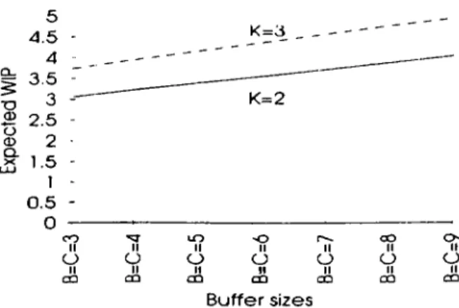
.As a next step, to observe the effect of K, performance measures for

f\='2 and A'=3 are compared. These are illustrated in figures 3.7 to 3.9. For

rhe case of A'=3. utilization of the machines is higher than that of A'= 2 case. This is expected because as the number of phases is increased, the part spends more time on each machine keeping it busy. Furthermore, utilizations of all machines are almost equal again for both cases. Mean throughput drops when we increase A' since the time it takes for a part to be processed through the t ransfer line increases, causing the number of parts produced per time to fall. Expected value of WIP is greater when K increases. On the other hand, variance of WIP decreases as the number of stages of the Erlang distribution is incn'ased. That is. when K is increased, more WIP is carried, but the deviation froiu this value is less. Hence, if the aim is to keep a stable WIP level, although it may be a little bit high, smaller K values should be chosen.

In order to see the effect of buffer sizes, we investigate the performance nu'asures for the case when the size of one of the buffers is fixed and the other is varied. The results of different problems are represented in tables 3.1. to 3.22. Whereas, we only provide the graphs for the cases B= I, and C is varied, ("= 1, and B is varied; 5 = 5 , and C is varied, C =o, and B is varied: 5 = 6 . and

C is varied, C = 6. and 5 is varied. These graphs are given in figures 3.10. to

3.18. For all cases, utilization is almost equal for the case where C is fi.xed, 5 is varying and the case where 5 is fixed, C is varying. For all performance measures, the following is observed. When the size of one of the buffers is set to a. constant value, c, and the size of the other buffer is varied, the performance

CHAPTER 3. EXPERIMENTAL RESULTS 31

measure is better until the point where B = C = c for the case where B is fixed and C is changing, and after that point performance measures are better for the case where C is constant and B varies. Another observation is that for the case where C is constant, and B is varied, performance measures are always around a stationary value. Whereas, for the opposite case, although the utilization and mean throughput are almost constant, expected WIP increases linearly while variance of W IP exhibits an exponentially increasing behaviour as dis­ cussed previously. Moreover, although buffer sizes are increased, throughput stays almost the same for both cases. Hillier and So [24] prove that percent­ age increases in throughput decrease as buffer capacities increase. Hence, our finding also supports this observation.

The.se observations lead to the following observation. If the processing rates of the machines are equal and if there is restricted available space for buffers, i.e. when a total amount must be allocated between the two buffers, the first buffer always should get more if we want to reduce the expected value of WIP and the variance of it. For example, if the total available space is 12 parts for A'=3, A = l/unit time, /q = ^2 = /íз=2/l·ınit time case, 5 = 9 . C=3 coml)ination gives an expected WIP value of 3.73741 and a variance value of 0.2')'>79. However, 5 = 8 , C=4 gives 3.95295 and 1.35911 respectively. Finally, 5 = 7 . C'=5 gives 4.16362 and 2.79884 respectively.

Finally, we try 0 processing rate combinations, such as /¿1 < /¿2 < /¿3? //i > /ii > /¿3, > p2 < /¿3, and /¿1 < Hi > /¿3 . Obviously, the utilization

of the machines are higher for smaller processing rates. For /¿i < /¿2 < /«3, we performed experiments to see the effect of changing buffer sizes. .Again until the intersection point, performance measures are better for the case where C is constant and 5 is varying. .All the previous discussion related to changes in buffer sizes for constant processing rates are also valid for < /¿2 < /ts and others. It is worth in noting that expected value of WIP is again a linear function of buffer size while the variance of WIP is increasing exponentially with the increasing buffer size. The plots of these experiments are given in figures 3.19. to 3.20.