Wide-area damping of power system oscillations using model predictive control

YAŞAR UNIVERSITY

GRADUATE SCHOOL OF NATURAL AND APPLIED SCIENCES MASTER THESIS

WIDE-AREA DAMPING OF POWER SYSTEM

OSCILLATIONS USING MODEL PREDICTIVE

CONTROL

Munir Aminu HUSEIN

Thesis Advisor: Assist. Prof. Emrah BIYIK

Department of Electrical and Electronic Engineering

İZMİR, TURKEY 2014

i

I certify that I have read this thesis and that in my opinion it is fully adequate, in scope and in quality, as a dissertation for the degree of master of science.

Assist. Prof. Dr. Emrah BIYIK (Supervisor)

I certify that I have read this thesis and that in my opinion it is fully adequate, in scope and in quality, as a dissertation for the degree of master of science.

Assist. Prof. Dr. Hacer SEKERCI

I certify that I have read this thesis and that in my opinion it is fully adequate, in scope and in quality, as a dissertation for the degree of master of science.

Assist. Prof. Dr. Erginer UNGAN

___________________________________ Prof. Dr. Behzat GÜRKAN Director of the Graduate School

ii

ABSTRACT

Electromechanical oscillations in power systems have been observed ever since synchronous generators were interconnected to provide reliability and higher generation capacity, and have become a severe threat for the safe and economic operation of modern interconnected power grids. With the development of wide-area measurement system (WAMS) and deployment of synchronized Phasor Measurement Units (PMU), Wide-Area Damping Controller (WADC) is designed to enhance the damping of these oscillations.

This thesis develops a systematic procedure of designing Wide-Area Damping Controller (WADC) using Model Predictive Control (MPC) technique to damp electromechanical oscillations in power system. The proposed technique is based on a linearized discrete-time state space model of a power system. The MPC controller computes the optimal input sequence over a chosen time horizon by solving a quadratic programming problem and sends these signals to the excitation system of a remote generator where it will supplement the local damping controllers. Power System Stabilizers were used as local damping controllers in this thesis.

The effectiveness and robustness of the proposed Model Predictive Controller for wide-area damping control scheme have been verified by two study systems. The first test system is the IEEE 4-Generator 2-Area test system. The second one is the IEEE 16-Generator 5-Area test system.

Simulation results of these test systems reveal that the proposed MPC wide-area damping controller damps the inter-area oscillations effectively under varying operation conditions and different disturbances.

Keywords: Power System, Model Predictive Control, Inter-area Oscillations, Wide-area

iii

ÖZET

Güç sistemlerinde güvenli ve yüksek kapasitede güç üretimi sağlayan senkron jeneratörler elektromekanik salınımlara sebep olmaktadırlar. Bu salınımlar kimi durumlarda modern elektrik şebekelerinin güvenli ve ekonomik işletilmesini tehdit eder boyuta gelmektedirler. Geniş Alan Ölçüm Üniteleri (WAMS) ve Senkronize Faz Ölçüm Uniteleri’nin (PMU) yaygınlaşması ile birlikte bu salınımları sönümlemek için Geniş Alan Baskılama Denetleyicilerinin (WADC) tasarımları mümkün olmaya başlamıştır. Bu tezde, güç sistemlerinde alanlar arası salınımları sönümlemek için Model Öngörümlü Denetleç (MPC) yöntemini kullanan bir Geniş-Alan Baskılama Denetleyicisi tasarlanmıştır. Önerilen yöntem, güç sistemlerinin lineer kesikli zamanlı durum uzayı modelini temel almaktadır. MPC denetleyici belirli bir tahmin ufku içerisinde en iyi kontrol sinyalini Karesel Programlama problemini çözerek hesaplamakta ve sonrasında bu sinyalleri uzaktaki jeneratörlerde bulunan yerel salınımları sönümleyici denetleyicilere ek kontrol sinyali olarak göndermektedir. Bu tezde yerel salınımları sönümlemek için Güç Sistemi Kararlı Kılıcısı (PSS) kullanılmaktadır.

Tasarlanan MPC denetleyici önce ideal durumda test edilmiş (bütün durum değişkenleri gözlenebilir ve kontrol edilebilir, haberleşme ve hesaplama gecikmeleri ihmal edilebilir Kabul edilerek), sonrasında, önerilen metodun durum değişkeni tahmin hataları ve hesaplama ve haberleşme gecikmelerinin olduğu durumlardaki etkinliği değerlendirilmiştir.

Önerilen denetleyicinin etkinliği ve gürbüzlüğü iki ayrı test sistemi üzerinde teyit edilmiştir. Ele alınan ilk system IEEE 4-jeneratör, 2-Alan test sistemi, ikincisi ise IEEE 16 Jeneratör, 68 Baralı test sistemidir. Bu test sistemleri üzerinde yapılan benzetim çalışmaları sonucunda MPC denetleyicinin değişken çalışma koşullarında ve farklı bozucu etkilere karşı geniş alan salınımlarını başarıyla sönümlediği, ve ayrıca geniş-alan sinyallerindeki gecikmelere karşı gürbüz olduğu gözlemlenmiştir.

Anahtar kelimeler: Güç sistemleri, Model öngörümlü denetleç, Alanlar-arası

iv

ACKNOWLEDGEMENTS

I would like to express my deepest gratitude to my research advisor, Assist. Prof. Dr. Emrah Biyik, for his patience, support and guidance throughout my MSc research. It has been a privilege for me to work under his supervision and I am his student forever. I thank the members of my thesis committee, Assist. Prof. Dr. Hacer SEKERCI and Assist. Prof. Dr. Erginer UNGAN, for devoting their time to read this manuscript and providing useful feedback.

I also wish to extend my sincerest appreciation to the entire staff of Electrical and Electronic Engineering of Yasar University, for their support throughout my studies. Many thanks to Prof. Mustafa Gunduzalp and Assoc. Prof. Mustafa Secmen for their invaluable guidance.

I acknowledged the help and support I received from Smart Grid Lab of Kookmin University, South Korea. Special thanks go to Prof. Il Yop Chung, his enthusiasm is a strong source of inspiration.

I thank my brother and classmate, Habibu Aminu Husein, and the rest of my family and friends, who have sustained and supported me in my endeavors for so many years. I feel so lucky to have been blessed with them.

Munir HUSEIN İzmir, 2014

v

TEXT OF OATH

I hereby declare that this thesis is my own work and that, to the best of my knowledge and belief, it reproduces no material previously published or written or material which has been accepted for the award of any other degree or diploma, except where due acknowledgement has been made in the text.

_________________

vi TABLE OF CONTENT Page ABSTRACT ii ÖZET iii ACKNOWLEDGEMENTS iv TEXT OF OATH v TABLE OF CONTENTS vi INDEX OF FIGURES ix INDEX OF ABBREVIATIONS x INDEX OF SYMBOLS xi CHAPTER 1. INTRODUCTION 1

1.1 Background and Motivation 1

1.2 Literature Review on Wide Area Damping Control 3

1.3 Thesis Organization 5

CHAPTER 2. OVERVIEW OF MODEL PREDICTIVE CONTROL 7

2.1 What is Model Predictive Control? 7

2.2 Model Predictive Control Strategy 7

2.3 Components of Model Predictive Control 9

2.3.1 Predictive Model 10

2.3.2 Objective Function 10

2.3.3 Obtaining the Control Law 11

2.4 Mathematical Formulation of MPC 11

2.5 Advantages and Disadvantages of MPC 16

vii

TABLE OF CONTENT (CONT.)

2.7 Review of MPC Applications in Power System 18

CHAPTER 3. MPC WIDE-AREA DAMPING CONTROL DESIGN 21

3.1 Outline of the Design Procedure 21

3.2 MPC Wide-area Damping Controller Architecture 22

3.3 Power System Modeling 23

3.4 Linearized State Space Model of Power System 29 3.5 Modal Analysis and Small Signal Stability 33

3.6 Controller Synthesis 35

CHAPTER 4. CASE STUDIES 39

4.1 Introduction 39

4.2 IEEE 4-Generator 2-Area Test System 39

4.2.1 Test System Description 40

4.2.2 Full-order Model and Small Signal Analysis 40 4.2.3 Structure of the Proposed MPC Wide-area Damping 43

4.2.4 Control objectives and constraints 44

4.2.5 Controller Synthesis 45

4.2.6 Simulation and Results 46

4.3 IEEE 16-Generator 5-Area Test System 49

4.3.1 Test System Description 49

4.3.2 Full-order Model and Small Signal Analysis 50

4.3.3 Control Objectives and Constraints 53

4.3.4 Controller Synthesis 54

viii

TABLE OF CONTENT (CONT.)

CHAPTER 5. CONCLUSION AND FUTURE WORK 62

5.1 Conclusion 62

5.2 Future Work 63

BIBLIOGRAPHY 64

APPENDIX

Appendix A IEEE 4-Generator 2-Area Test System Parameters 73 Appendix B IEEE 16-Generator 5-Area Test System Parameters 77

ix

INDEX OF FIGURES

Page Fig. 2.1 Basic Model Predictive Control Strategy 8

Fig. 2.2 Basic Structure of MPC 10

Fig. 3.1 Architecture of MPC Wide-area Damping Control 23 Fig. 3.2 Synchronous Generator Schematic Diagram 24

Fig. 3.3 IEEE DC1A Exciter Block Diagram 26

Fig. 3.4 Govornor Model Block Diagram 28

Fig. 3.5 Power System Stabilizer Block Diagram 28

Fig. 4.1 IEEE 4-Generator 2-Area Test System 39

Fig. 4.2 Calculated Modes of IEEE 4-Generator 2-Area Test System 42 Fig. 4.3 Compass Plot of Rotor Angle Terms of Inter-area Mode 43

Eigenvector

Fig. 4.4 Configuration of Generator Participating in MPC Wide-area 44 Damping

Fig. 4.5 Speeds of all 4 Generators with PSS (No MPC) 46 Fig. 4.6 Speed of all Generators with the proposed MPC Wide-area 47

Damping

Fig. 4.7 MPC Wide-area Control Signals for 4 Generators 48 Fig. 4.8 IEEE 16-Generators 5-Area Test System 49 Fig. 4.9 Calculated Modes of IEEE 16-Generator 5-Area Test System 51 Fig. 4.10 Compass Plot of Rotor Angle Terms of Inter-area Mode 53

Eigenvector

Fig. 4.11 Speeds of 16 Generators with only PSS (No MPC) 56 Fig. 4.12 Speeds 16 Generators with both PSS and MPC Controller 57 Fig. 4.13 MPC Wide-area Signals to Generators 1, 2, 11 and 12 58

Fig. 4.14 Speed of Generator 1 59

Fig. 4.15 Speeds of all Generators with PSS (No MPC) 60 Fig. 4.16 Speeds of all Generators with both PSS and MPC 61

x

INDEX OF ABBREVIATIONS

MIMO Multi-Input Multi-Output MPC Model Predictive Control

SCADA Supervisory Control And Data Acquisition EMS Energy Management System

WAMS Wide Area Measurement System PMU Phasor Measurement Unit

GPS Global Positioning System WADC Wide Area Damping Controller SISO Single-Input Single-Output PSS Power System Stabilizer

FACTS Flexible AC Transmission Systems LMI Linear Matrix Inequality

WACS Wide Area Control System

WECC Western Electric Coordinating Council LPSS Local Power System Stabilizer

xi

INDEX OF SYMBOLS

Symbols Explanations

A State matrix of state-space model

B Input-to-state matrix of state-space model C State-to-output matrix of state-space model Sampling time

MPC control time step

Cost function for optimization Control horizon

Prediction horizon

Weighting factor for control increments

Weight on manipulated variable Weighting factor for predicted error Generator speed

Generator rotor angle

Generator field voltage

Direct and quadrature axis components of stator voltage _{Direct axis synchronous, transient and subtransient reactances Quadrature axis synchronous, transient and subtransient reactances Direct and quadrature axis air gap flux linkage}

Direct and quadrature axis amortisseur circuit flux linkage

Power system states and estimated states Measured and estimated output

Exciter reference voltage Output reference

1

CHAPTER 1

INTRODUCTION

1.1 Background and Motivation

Electric power systems are among the largest structural achievements of man. Electro-mechanical oscillations between interconnected synchronous generators are phenomena inherent in these systems [1]. The stability of these oscillations is of immense importance, and is a prerequisite for stable and secure system operation. If not damped out quickly, these oscillations may lead to generator outages, line tripping, network splitting and even blackouts [2]. In terms of oscillation ranges and frequencies, electromechanical oscillations can be divided into two categories, local mode oscillations and inter-area mode oscillations.

Local mode oscillations, also called plant mode, occur when a generator (or group of generators) at a station is swinging against the rest of the system. These oscillations have frequencies in the range 0.7 to 2.0 Hz [3]. The characteristics of these oscillations were understood, they were studied adequately, and satisfactory solutions to their stability problems were well developed.

Inter-area modes are associated with the swinging of many generators in one part of the system against generators in other parts. Their frequencies are in the range 0.1 to 0.7 Hz [3]. The characteristics of these modes of oscillations, and the factors influencing them, are far more complex to study, and to control. A detail representation of the entire interconnected system is required to study inter-area mode [4]. This thesis deals with inter-area oscillations.

Heavy power transfer across weak tie-lines or high-gain exciters are the main cause of Inter-area oscillations [3]. Large power systems typically exhibit multiple dominant inter-area swing modes, which are associated with the dynamics of power transfers and involve groups of machines oscillating relative to each other. When present in a power

2

system, these oscillations limit the amount of power transfer on the regions containing the groups of coherent generators [4].

In recent times, many instances of unstable oscillations, involving inter-area modes in large power systems have been observed, both in studies and in practice: at 0.6 Hz in the Hydro-Quebec system [5], at 0.2Hz in the western North-American interconnection [6], at 0.15-0.25 Hz in Brazil [7] and at 0.19-0.36 Hz in the UCTE/CENTREL interconnection in Europe [8]. The recent 2003 blackout in eastern Canada and US was accompanied by severe 0.4 Hz oscillations in several post-contingency stages [9]. In China, within the year 2008, two system-wide low-frequency oscillations incidences occur respectively in the South China and Central China grids [10].

Many other incidents of system outage resulting from these oscillations have been reported over the years, and as such, they are increasingly becoming a cause of concern. This has led to a renewed effort in understand the nature of these oscillations, methods for systematically studying them, and control techniques by which they can be stabilized.

The traditional control approach in use today to damp these oscillations is to employ conventional Local Power System Stabilizers (LPSS) that provide supplementary control action through the generator excitation systems. In recent times, Supplementary Modulation Controllers (SMC) are added to Flexible AC Transmission Systems (FACTS) devices to damp inter-area oscillations. These controllers are effective in damping local modes, and if carefully tuned [11] may also damp inter-area modes up to a certain transmission loading. Their effectiveness in damping inter-area mode is limited because these controllers are single-input single-output non-coordinated controllers that usually use local inputs and cannot always be effective in solving the problem due to two main shortcomings.

First, these local controllers are designed to have fixed parameters derived from linearized model around a certain nominal operating point. Therefore conventional local

3

controllers designed by classical control techniques have their validity restricted to a neighborhood of this point. But power systems constantly experience changes in operating conditions due to variations in generation and load patterns. Furthermore, some uncertainty is inevitably introduced into a power system model due to inaccurate approximation of the power system parameters, neglected high frequency dynamics and invalid assumptions made in the modeling process.

Second, it has been proven that under certain operating conditions, an inter-area mode may be controllable from one area and be observable from another [12]. In such cases, local controllers lack global observation of inter-area modes and hence are not effective for the damping of that mode.

The recently developed Wide-Area Control System (WACS) technologies offer a great potential to overcome the shortcomings of conventional local controllers in damping inter-area oscillations. With the fast development of global positioning system (GPS) based Phasor Measurement Units (PMU), dynamic data of power systems, such as voltage, current, angle, and frequency are reliable available and can be accurately measured, synchronized and transferred in the range of the whole power system by Wide-Area Measurement Systems (WAMS) [13, 14].

This advancement makes possible the construction of wide-area damping control systems. In contrast to conventional local controls, wide-area damping controls have many benefits. Reference [15] shows that wide-area damping controls are more efficient than local controls in preventing loss of synchronism and local controls need large gain (from 4 to 20 times more) than wide-area damping controls [16] to achieve a similar damping effect.

1.2 Literature Review on Wide Area Damping Control for Power System

Wide-area control refers to any control that requires some communication link to either gather the input or to send out control signals [17]. Although control using signals obtained remotely requires additional communication equipments, it is likely that the

4

cost of such equipment would be offset by additional operating flexibility gained by the control.

Many researchers achieved good results by applying wide area measurement to the design of wide-area control system for power system oscillation damping. One promising approach is to design wide-area measurement based controllers that provide control actions through generator excitation systems supplemental to the action of local PSS.

Wide-area damping controllers were perhaps first designed by Magdy et. al. [12]. They found that if wide-area signals are applied to the local controllers, the system dynamic performance can be enhanced with respect to inter-area oscillations.

Kamwa, Grondin and Hebert [18] propose a decentralized/hierarchical structure for a wide-area control system. Wide-area signals based PSS is used to provide additional damping to local ones. A sequential optimization procedure is used to tune the global and local loop of the proposed controller.

In [19], a systematic procedure of designing a wide-area controller is presented. The synthesis of the controller is defined as a problem of mixed H2/ H∞ output-feedback control with regional pole placement and is resolved by the linear matrix inequality (LMI) approach.

Reference [20] uses multi-agent concepts to coordinate several supervisory PSSs (SPSS) based on remote signals and exchanging information with local PSSs to improve power systems stability. The SPPs is designed by H∞ optimization methods. Rule based

fuzzy-logic and robust control techniques are used to deal with uncertainties introduced by nonlinear terms and operating conditions.

Defining the differences between post-fault transmission power and its steady state value as a cost function, paper [21] optimizes TCSC parameters based on sensitivity analysis to provide the maximum damping for various operation conditions. Paper [22] introduces angular speeds of remote generators to a PSS to improve its damping to inter-area oscillations.

5

As can be seen from the above works, various control techniques were used in designing these controllers. In recent years, Model Predictive Control (MPC) was found to be an attractive control algorithm for designing wide-area damping controllers. At a control instant, the MPC algorithm computes an open-loop sequence of inputs in order to optimize future plant behavior. The first input in the optimal sequence is injected into the plant, and the entire optimization is repeated at subsequent control steps [23].

This powerful control technique will be employed in this thesis to design wide-area damping controller to damp out inter-area oscillations in power systems.

1.3 Thesis Organization

The thesis is organized in five chapters. A brief summary of the chapters are as follows: Chapter 1 starts with the background and motivation of the thesis. A literature review that summarizes the research in wide-area damping control is presented. Finally, the organization of the thesis is presented.

Chapter 2 introduces Model Predictive Control, its strategy, algorithms, and applications. Its advantages and disadvantages are outline. Finally, review of MPC applications in power system is discussed.

Chapter 3 presents the procedure for designing wide-area MPC controller to damp inter-area oscillations in power system. A complete power system, including synchronous generator, excitation system, governor and power system stabilizer are then modeled. The proposed MPC scheme is outline, with detail state space representation, prediction formulation, and cost function optimization.

Chapter 4 provides two case studies to illustrate the effectiveness of wide-area MPC controller in damping power system oscillations. The first case study uses IEEE 4-Generator 2-area Test System, and the second uses IEEE 16-4-Generator 5-Area Test System.

6

Chapter 5 concludes the work, summarizing the findings as well as contribution related to the procedures in this thesis. Furthermore, possible future research topics were suggested.

Additionally, this thesis includes three appendices. Appendix A and B provide the dynamic data of IEEE 4-Generator 2-area Test System and IEEE 16-Generator 5-Area Test System respectively. Appendix C is a brief introduction of Power System Toolbox (PST).

7

CHAPTER 2

OVERVIEW OF MODEL PREDICTIVE CONTROL

2.1 What is Model Predictive Control?

Model Predictive Control (MPC), also referred to as ‘Receding Horizon Control’ and ‘Moving Horizon Optimal Control’, is a form of control in which a performance index is optimized with respect to some future control sequence, using predictions of the output signal based on the system model, while satisfying constraints on inputs and output/states.

The name ‘Model Predictive Control’ is from an idea of employing an explicit model of the plant to be controlled which is used to predict the future output behavior.

2.2 Model Predictive Control Strategy

Model Predictive Control, MPC, usually contains the following three ideas [24]:

(i) Explicit use of a model to predict the system output along a future time horizon

(ii) Calculation of a control sequence to optimize a performance index

(iii) A receding horizon strategy, so that at each instant the horizon is moved towards the future, which involves the application of the first control signal of the sequence calculated at each step

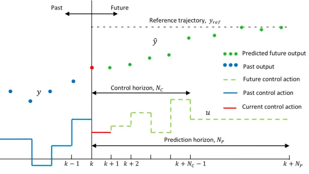
The methodology of all the controllers belonging to the MPC family is characterized by the following strategy illustrated as shown in Fig. 2.1.

8

Fig. 2.1 Basic Model Predictive Control Strategy

The strategy is described as follows:

 At each instant , the model is used to predict the future outputs, were (a finite integer ) is called the prediction horizon. These depend upon the known values up to instance (past inputs and outputs), including the current output (initial condition) and on the future control signals to be calculated. (Note – the notation indicates the value of at time instant calculated at instant ).

 At the current sampling instant, k, the MPC strategy computes a set of control moves . The number of these control moves,

is called control horizon. These moves were held constant after . The

objective of the MPC control computations is to determine a sequence of control moves so that the predicted outputs, , reaches the set point , in an optimal manner. These control moves are obtained by

Control horizon, Prediction horizon, Past Future Reference trajectory, Past output

Future control action Past control action Predicted future output

9

optimizing an objective function. The objective function usually takes the form of a quadratic function of the errors between the predicted output signal and the predicted reference trajectory. If the criterion is quadratic, the model is linear, and there are no constraints, an explicit solution can be obtained; otherwise an iterative optimization method has to be employed.

 Only the current control signal is transmitted to the plant. At the next sampling instant is measured and step 1 is repeated and all sequences brought up to date. Thus is then calculated using the receding horizon approach. The receding horizon concept is a distinguishing feature of the MPC. Although a sequence of control moves is calculated at each sampling instant, only the first move is actually implemented while ignoring the rest of the sequence. Then a new sequence is computed at the next sampling instant, after new measurements become available; again only the first input move is implemented. This process is repeated at each sampling instant.

2.3 Components of Model Predictive Control

Three components are common to all Model Predictive Controllers [24], and there are several options of representing each components resulting in different MPC algorithms. These components are:

 Prediction Model  Objective Function

 Obtaining the Control Law

In order to explain the function of each component, a basic MPC structure is shown in Fig. 2.2.

10

Fig. 2.2 Basic Structure of MPC (Modified from [24])

2.2.1 Prediction Model

The model is the cornerstone of MPC; model selection is the most important part of MPC design [25]. A model of the system is used to predict the future plant outputs, based on past and current values and on the proposed optimal future control actions. These actions are calculated by the optimizer taking into account the cost function as well as the constraints.

The model must be able to capture the system’s dynamics to accurately predict the future outputs and at the same time be intuitive and simple to implement and analyzed.

2.2.1 Objective Function

The optimizer is another crucial part of the MPC strategy as it provides the control actions. Various MPC algorithms use different cost function for obtaining the control law. Selection of the cost function is an area of both engineering and theoretical judgment. The main aim is for the future output (y) on the considered horizon follow a determined reference trajectory and at the same time the control effort ( )

necessary for doing so should be penalized.

Predicted outputs, - + Reference trajectory, Future errors Future inputs Past (inputs and outputs)

Cost function Constraints MODEL

11

2.2.3 Obtaining the Control Law

To obtain the values of it is necessary to minimize an objective function, . To obtain this the value of predicted outputs are calculated as a function of past values of inputs and outputs and future control signals, making use of the model chosen and substituted in the cost function, obtaining an expression whose minimization leads to the looked-for values. An analytical solution can be obtained for the quadratic criterion if the model is linear and there are no constraints, otherwise an iterative method of optimization should be used.

2.4 Mathematical Formulation of MPC

There are many different types of models used in MPC formulation, the choice depend on which algorithm is employed. Recent years have seen the growing popularity of predictive control design using state-space design methods [26], therefore a linearized, discrete-time, state-space model will be used in this section to derive MPC prediction equations, objective functions and constraints.

Consider the linearized, discrete-time, state-space model of the plant, in the form:

(2.1)

where is a -dimensional state vector, is a -dimensional input vector, is a -dimensional measured output vector, and is a -dimensional vector of output which are to be controlled, either to particular set-points, or to satisfy some constraints, or both. The index counts ‘time steps’. The variables in and usually overlap, and frequently are the same; meaning all the controlled outputs will frequently be measured. Often, it will be assumed that , and C will be used to denote both and .The index counts ‘time steps’. Equation 2.1 can then be simplified to:

12

(2.2)

(2.3)

In practice, it should not be assumed that all states variables can be measured directly and exactly, so an estimated will be used to replace the real state, . Correspondingly, and denote the predictions of variables x and y at time k + 1, on the assumption that one input is applied at time k. So, Equation (2.2) and (2.3) can be further changed to:

(2.4)

(2.5)

The predictions can now be made of a future states over a given prediction horizon, , by iterating Equation (2.4) and (2.5)

(2.6) . . .

13

The above equations can be expressed in the matrix-vector form: (2.7)

The input vector changes only at the first steps, namely at the times and will remain constant thereafter. That is to say, for . The items in the input matrix corresponding to the same in Equation (2.7) to obtain:

(2.8)

In the predictive control, the input change is often computed rather than Defining that (2.9)

14 (2.10)

Finally, the predictions of y over the whole prediction horizon are given by: (2.11)

Equation (2.10) and (2.11) can be written as

(2.12) (2.13) where:

15

Based on the above prediction equations, the MPC seeks for an optimal sequence of which minimizes a given cost function. A typical cost function is given in Equation (2.14). It penalizes the deviation of the predicted controlled output from a reference trajectory and the input change

The reference trajectory may be some predetermined trajectories.

The prediction horizon has length but is not necessary to start penalizing deviation of from immediately because there may be some delay between applying an input and seeing any effect. and are weight matrices. The solution minimizing Equation (2.14) should be subject to the following constraints:

(2.15) (2.16) (2.17) The constraints were assumed to hold over the control and prediction horizons. E, F and G are matrices of suitable dimensions. denotes a column vector, each of which is zero. These constraints can be used, for example, to represent possible actuator slew

16

rates (2.15), actuator ranges (2.16), and constraints on the controlled variables (2.17). When solving MPC optimization problem, all the above inequalities must be translated into the inequality concerning namely

Here, E is a coefficient matrix of proper dimensions.

2.5 Advantages and Disadvantages of MPC

MPC has the following main advantages [24]:

 Concepts are intuitive and attractive to industry

 Can be used to control a great variety of processes, including those with non-minimum phase, long time delay or open-loop unstable characteristics

 Can deal with multivariable, multi-input multi-output as well as single-input single-output process

 Constraints on inputs and outputs are considered in a systematic manner

 Readily applicable to batch processes where the future reference signals are known

 An open technology which allows for future extensions

 Accurate model predictions can provide early warning of potential problems Significant disadvantages are:

 Requirement of an appropriate model of the process, which may be difficult to obtain for some complex systems

 Computationally demanding if the optimization problem is not formulated properly

17 2.7 MPC History and State of the Art

The MPC concept has a long history. Its current industrial and academic interest can be traced back to a set of papers which appeared in the late 1970s. In 1978 Richalet et al. [27] describes successful applications of “Model Predictive and Heuristic Control” and in 1979 engineers from Shell (Cutler and Ramaker [28]; Prett and Gillette [29]) outlined “Dynamic Matrix Control” and reported applications to a fluid catalytic cracker. In both algorithms an explicit dynamic model of the plant is used to predict the effect of future actions of the manipulated variables on the output (thus the name Model Predictive Control). The future moves of the manipulated variables are determined by optimization with the objective of minimizing the predicted error subject to operating constraints. The optimization is repeated at each sampling time based on updated information (measurements) from the plant.

Even though the above two works sparked the current interest in MPC, what have since become recognized as the central MPC concepts actually predates these first reports of application by some twenty years [30]. Zadeh and Whalen [31] first recognize the connection between the closely related minimum time optimal control problem and linear programming. The first publication to explicitly introduce the now standard MPC concept seems to be Propoi [32], who proposed in 1963 the moving horizon approach which is an essential part of all MPC algorithms. It became known as “Open Loop Optimal Feedback”. During the 1970s, Gutman [33] reviewed much of the extensive work in this area. The connection between this work and MPC was discovered by Chang and Seborg [34].

Garcia and Morari [35] were perhaps the first to attempt placing the MPC within the same framework as the so-called “classical Control”, in which the Internal Model Control (IMC) paradigm was proposed. They showed that the IMC structure – in which an internal model of the plant operates in parallel with the plant, and in which the controller is some appropriate inverse of this plant model – is inherent in all MPC scheme. This and subsequent publications by Morari and coworkers provided insight into the stability, robustness and performance of MPC scheme [36, 37].

18

Keyser et al. [38] presented a comparative study of self-adaptive long range predictive control (LRPC) technique while keeping focus on robustness with respect to unmodeled dynamics, parameter variations, process noise and varying dead-time. Scattolini and Bittanti [39] produce some simple criteria stated in terms of the plant step or impulse response for the selection of prediction horizon. This selection is important as it guarantees the closed-loop stability.

In 1991, Scattolini and Clarke [40] found that constrained receding horizon predictive control optimizes a quadratic function over a costing horizon to stabilize general linear plants. The computation is more complex, however. An alternative is to employ finite-horizon techniques, which are numerically very sensitive.

In 1999, Morari and Bemporad [41] investigate robustness in MPC and proposed techniques for stability, performance and constraint handling. Joe Qin and Badgwell [42] came up with an overview of commercially available MPC technology. They reported wide application of MPC in industrial applications.

Nonlinear MPC based on state space models and the receding horizon concept has also been developed, for example by Mayne and Michalska [43], who perform a stability analysis, and Balchen, Ljungquist and Strand [44]. Becerra, Roberts and Griffiths [45] integrate an economic objective within the performance function.

In 2007, Dubay and Ayyad [46] provided real time comparison of a number of predictive controllers.

2.8 Review of MPC Applications in Power Systems

MPC presents a dramatic advancement in the theory of modern automatic control [47]. It was originally studied and applied in the process industry, where it has been in use for decades [48]. An MPC survey by Qin and Badgwell [42] reported that there were over 4,500 applications worldwide by the end of 1999, primarily in oil refineries and petrochemical plants. In these industries, MPC has become the method of choice for difficult multivariable control problems that include inequality constraints.

19

In view of its remarkable success, a question to be answered is, why is MPC, hitherto, not extensively applied to control other systems, such as electrical power systems? This is as a result of two short comings. First, MPC needs an accurate model of the system, and this is not usually a simple task. Secondly, computational burden of MPC increases exponentially. These shortcomings were, however, solved as a result of availability of very good mathematical models and powerful microprocessors that can perform the large amount of computations needed in MPC at a high speed and reduced cost.

These advancements lead to a growing application of MPC in other areas. In the field of power systems, for example, it finds applications in power electronics [49, 50, 51], frequency control [52, 53], voltage control [54, 55], power system transient stability [56, 57], power system protection [58, 59], and smart-grids [60, 61], among others.

In recent years, MPC is extensively employed by researchers to design wide-area damping controller to damp out inter-area oscillations in power system.

Paper [62] introduces a new MPC scheme to damp wide-area electromechanical oscillations in power system. The proposed MPC controller, based on a linearized discrete-time state space model, calculates the optimal input sequence for local damping controllers over a chosen time horizon by solving a quadratic programming problem. Distributed Model Predictive Control was investigated in reference [63] to damp wide-area electromechanical oscillations. This distributed MPC scheme is derived from and compared with a fully centralized MPC scheme proposed in [62].

An efficient adaptive stability control for multi-generator power system is presented in [64] based on step-ahead model prediction methodology. Method of Equivalent Circuit (MEC) is proposed to design the Model Predictive Adaptive Controller (MPAC) excitation for multi-generator power system by defining the deviation of predicted output from reference and control input increment as an objective function

In [65], a wide-area damping supplementary inter-area controller, using the reduced order state space model with dominant low frequency oscillations modes obtained by

20

system identification, based on model prediction and sliding mode variable structure control, was designed to damp the inter-area low frequency oscillations in power system.

21

CHAPTER 3

MPC WIDE-AREA DAMPING CONTROL DESIGN

3.1 Introduction

This chapter presents the design methodology of wide-area MPC damping controller. The following are the steps taken in the design proposed in this thesis:

Step 1. Full-order nonlinear model of the test system: The multi-machine dynamic model of the test system is calculated using Power System Toolbox [66]. All generators are represented by the detail model, i.e. two-axis model with exciter, governor and conventional power system stabilizers.

Step 2. Model linearization: The full-order nonlinear model is linearized at a chosen operating point. This is necessary since the proposed MPC controller requires a linear model for its predictions.

Step 3. Modal analysis and small signal stability: Once the linearized model of the system is obtained, the small signal stability analysis can be computed and analyzed. The eigenvalues and eigenvectors are determined to get the frequencies and damping ratios of local and inter-area modes.

Step 4. Controller Synthesis: An MPC technique is used to calculate the optimal input sequence and send these signals to each generator excitation system. MATLAB MPC Toolbox is used to design the controller. The designed controller should meet the requirement of stability and provide acceptable damping to inter-area oscillations.

Step 5. Simulation and results: The performance of the controller is evaluated in the closed-loop system with the full-order linear model using MATLAB.

22

3.2 MPC Wide-Area Damping Controller Architecture

The architecture of the proposed MPC wide-area damping controller is illustrated in Fig3.1. In most power systems, local oscillation modes are often well damped due to the installation of local PSS. Inter-area oscillation modes, on the other hand, are often lightly damped because the control inputs used by those PSS are local signals which often lack good observation of inter-area modes. This suggests that a wide-area controller, which uses wide-area measurements as its inputs to create control signals supplement to local PSSs, may help to improve the damping of inter-area oscillations. In real time, the wide-area MPC controller collects WAMS measurements measured by PMUs and sent to the MPC controller via dedicated communication link (WAMS). These measurements, of the system state (a state estimator would normally be needed) are collected at discrete measurement times (in this thesis . The MPC uses its model to compute an open loop sequence of the control variables u over a chosen control horizon . It sends these control signals computed for the first period of seconds to the excitation system of each generator. It then waits for the next measurements to be received in order to start this calculation again.

23

Fig. 3.1 Architecture of MPC Wide-area Damping Control Systems

3.3 Power System Modeling

In power systems, the primary sources of electrical energy are synchronous generators. The stability of the system depends on several other components such as excitation systems, speed governors, power system stabilizers, the loads etc. Therefore, an understanding of their characteristics and modeling of their performance are of fundamental importance for stability studies and control design. The general approach to modeling these components are quite standard. This section provides the detail of power system dynamic model used in this thesis.

+ + + + + + To other generators To other generators

Model Predictive Controller for Damping Wide-area Power Systems Oscillations

Exciter PSS Exciter PSS Phasor Data Concentrator PMU PMU

PMU Data Uploading PMU Data Uploading

One of the generators participating in inter-area oscillation mode, Area n

One of the generators participating in inter-area oscillation mode, Area m

MPC Wide-area Signals

24

3.3.1 Synchronous Generator Model

Synchronous generators form the principal source of electric energy in power system. The power system stability problem is largely one of keeping interconnected synchronous machines in synchronism. In this thesis, a sixth-order subtransient model, as described in [67] has been used.

Fig. 3.2 Synchronous Generator Schematic Diagram

The six dynamic equations that model the sixth-order subtransient synchronous generator in Fig. 3.2 can be stated as:

(3.1)

(3.2)

25 (3.3) (3.4) _(3.5) (3.6) where

δ generator rotor angle

ω generator rotor speed in per unit

J moment of inertia mechanical torque electromechanical torque damping coefficient

_{, direct and quadrature axis components of stator flux linkage} direct and quadrature axis transient stator voltage

direct and quadrature armortisseur circuit flux linkage

leakage reactance;

_{direct axis synchronous, transient and subtransient reactances; quadrature axis synchronous, transient and subtransient}

26

quadrature axis open circuit and subtansient time constants;

direct and quadrature axix stator current

excitation voltage and current

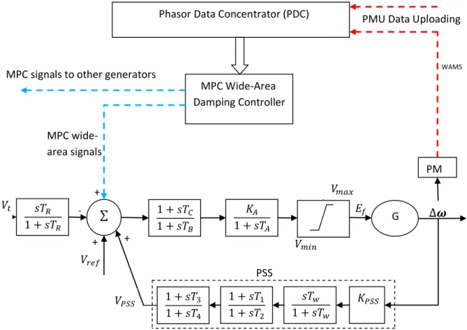
3.3.2 Exciter Model

When the behavior of synchronous machines is to be accurately simulated in power system stability studies, it is essential that their excitation systems be modeled in sufficient detail [68]. The basic function of an excitation system is to provide direct current to the synchronous machine field winding. In addition, the excitation system performs control and protective functions essential to the satisfactory performance of the power system by controlling the field voltage and thereby the field current. The desired models must be suitable for representing the actual excitation equipment performance for large, severe disturbances as well as for small perturbations.

IEEE Type DC1A Exciter [69] is used in this thesis. Its block diagram is shown in Fig. 3.3.

Fig. 3.3 IEEE DC1A Exciter Block Diagram [69]

+ - + - + -

27

The dynamics of this exciter can be represented by the following differential equations:

(3.7) (3.8) (3.9) where voltage deviation

exciter reference voltage regulator states

voltage regulator gain

voltage regulator time constant

transient gain reduction time constants

3.3.3 Governor Model

The prime mover governing systems provide a means of controlling the synchronous machine speed and hence voltage frequency. In order to automatically control speed and frequency, a device must sense either speed or frequency in such a way that comparison with a desired value can be used to create an error signal to take corrective action.

(3.10) _{(3.11) (3.12)} (3.13)

28

Fig. 3.4 Governor Model Block Diagram [67]

3.3.4 Power System Stabilizer Model

The basic function of Power System Stabilizer (PSS) is to add damping to the generator rotor oscillations by controlling its excitation using auxiliary stabilizing signal(s). To provide damping, the stabilizer must produce a component of electrical torque in phase with the rotor speed deviations. Fig. 3.5 illustrates the theoretical basis for a PSS with the help of block diagram. Since the purpose of a PSS is to introduce damping torque component, a logical signal to use for controlling generator excitation is the speed deviation. (3.14) (3.15) (3.16) (3.17)

Fig. 3.5 Power System Stabilizer Model Block Diagram [69]

+ _ _ + ω

29

3.3.5 Load Model

Modeling load in stability studies is complicated because a typical load bus is composed of a large number of devices such as fluorescent and incandescent lamps, refrigerators, heaters, compressors, motors, furnaces, etc. Therefore, load representation in system studies is based on a considerable amount of simplification.

Load can be either static or dynamic and can be modeled using constant impedance, constant current and constant power static load models. These loads can be described by the following polynomial equations [70]:

(3.18)

(3.19)

where and are the load real and reactive powers consumed under nominal conditions, i.e., at the reference voltage and the nominal frequency . and are the powers consumed by the load under current conditions of voltage and frequency . The value is a loading factor, which is an independent demand variable.

3.4 Linearized State Space Model of Power System

Although a real power system is a complex, nonlinear and high-order dynamic system, it can be represented by a relatively simple linear model with fixed structure but whose parameters vary with the operating conditions, which is accurate enough for the purpose of designing a damping controller.

The synchronous generator model along with the associated regulating devices thus becomes a fifteenth-order model (15 state variables for each synchronous machine). These dynamic states are:

30

3 Exciter states:

3 Governor states: 3 PSS states: The states vector is thus;

In the design proposed in this thesis, the control inputs to the power system are additional MPC wide-area signals added to each generator excitation system. The control inputs are:

where ng is the number of controlled generators.

The 15 differential equations describing each machine are:

31

The full dynamic behavior of the power system may be describe by a set of first order nonlinear differential equations as presented below

(3.20)

If the derivatives of the state variables are not explicit function of time, the system is said to be autonomous. In this case, Equation 3.20 simplifies to

(3.21)

Often, the variables of interest are output variables which can be observed on the system. These may be expressed in terms of the state variables and the output variables in the following form:

32

Let be the initial state vector and the input vector corresponding to the equilibrium point about which the small-signal performance is to be investigated. Since and satisfy Equation 3.21, then

(3.23)

Let’s perturb the system from the above state, by letting prefix denotes a small deviation.

The new state must satisfy Equation 3.21. Hence,

(3.24) As the perturbations are assumed to be small, the nonlinear function can be expressed in terms of Taylor’s series expansion. All the terms involving second and higher order powers of and are neglected, it can be written:

Since we obtain

With In a like manner, from Equation (3.22), it can be expressed:

33

With Therefore, the linearized forms of Equations (3.21) and (3.22) are (3.25) (3.26) where

The above partial derivatives are evaluated at the equilibrium point about which the small perturbation is being analyzed.

3.5 Modal Analysis and Small Signal Stability

Small signal stability of the power system can be calculated and analyzed once the power system is represented in general state space form as given in (3.25) and (3.26). Because each eigenvalues correspond to an oscillation mode of the system, small signal stability analysis is also referred to as modal analysis [67].

Small signal analysis establishes that the stability of a system equilibrium point under small disturbances can be studied by linearizing the nonlinear system equation around the system equilibrium point. Then, the system stability can be determined by inspecting the eigenvalues, of the system state matrix [71]. Eigenvalues are the non-trivial solutions of the equation:

34

where is an vector. Rearranging (3.25) to solve for yields

det (3.28)

The solution of (3.28) are the eigenvalues of the matrix of . These eigenvalues are of the form . The operating point is stable if all the eigenvalues are on the left-hand side of the imaginary axis of the complex plane; otherwise it is unstable. As a pair of complex eigenvalues crosses the imaginary axis, it is known as Hopf bifurcation [72].

The oscillation frequency in Hertz and damping ratio are given by:

(3.29)

(3.30)

In linear system, the dynamics can be described as a collection of modes. A mode is characterized by its frequency and damping and the activity pattern of the system states. The system matrix can be diagonalized by the square right modal matrix :

_(3.31)

The columns of are the right eigenvector to , while the diagonal elements of the diagonal matrix are the eigenvalues of . Similarly the left modal matrix holds the left eigenvector as rows and also diagonalizes .

_(3.32)

The right and left modal matrix are normalized so that:

(3.33)

The right eigenvector gives the mode shape, i.e., the relative activity of the state variables when a particular mode is excited. Its magnitude give the extent of the activities of the n state variables in the ith mode, and the angles of the elements give phase displacements of the state variables displays only the ith mode. The left

35

eigenvector identifies which combination of the original state variables displays only the ith mode.

3.6 Controller Synthesis

In this thesis, the real power system is replaced by nonlinear time domain simulation software, s_simu, from the MATLAB Power System Toolbox (PST) [66]. Next,

svm_mgen, which is a small signal stability analysis software also from PST, is used to

derive the linearized continuous time model

(3.34)

(3.35)

Where, is a vector of state variables, is vector of inputs, is a vector of outputs. The Equation (3.34) and (3.35) were then discretized using a transition for a small step of δ seconds to obtain a discrete-time dynamics

(3.36)

(3.37)

At time t, based on an estimation of the current system states (obtained from a state estimator), the predicted outputs over the next horizon are obtained by iterating Equation (3.36) and (3.37) times by using as the initial state. is the prediction horizon.

(3.38) (3.39)

36 where:

Based on the above prediction equations, the MPC seeks for an optimal sequence of which minimizes a given cost function. A typical cost function is given in Equation (3.40). It penalizes the deviation of the predicted controlled output from a reference trajectory and the input change The reference trajectory may be some predetermined trajectories:

The MATLAB MPC Toolbox is used to compute the solution of this quadratic programming problem. The first solution of this problem is sent to the excitation system of generators and the calculation is repeated at the next measurement step by using the measured state as input.

37

Controller Tuning

The following parameters need to be specified when designing MPC controller: : Prediction Horizon (number of predictions)

: Control Horizon (number of control moves) : Sampling period

: Weighting matrix for predicted errors

: Weighting matrix for manipulated variables rate

: Weighting matrix for manipulated variables

Although the values of these parameters are normally guided by heuristics, there are some general guidelines for their selection to ensure the optimization is well proposed.

1. Choice of Horizons Prediction horizon,

Predictive horizon should be selected to include all significant dynamics; otherwise performance may be poor and important events may be unobserved. The prediction horizon should be larger than control horizon plus the system settling time.

Control Horizon,

Increasing makes the controller more aggressive and increases computational effort, typically

The control horizon should be as large as the expected transient behavior.

Rossiter [25] summarizes the effects of varying these parameters:

 If is small, increasing causes the loop dynamics to slow down

 If is large, increasing improves performances

 If is large, then increasing improves performance

38

 As is increased, norminal closed-loop performance improves if is large enough

 As is increased nominal closed-loop performance improves if is large enough. However, for many models, there is no much change beyond

2. Weighting matrices , and

Choosing the weights is a critical step in MPC [73]. Usually, the controller weights needs to be tune in order to achieve the desired behavior. Diagonal matrices with largest elements correspond to most important variables

 Output weighting matrix : the most important variables having the largest weights

 Input weighing matrix (move suppression matrix) : increasing the values of weights tend to make the MPC controller more conservative by reducing the magnitudes of the input moves. Increasing slows

39

CHAPTER 4

CASE STUDIES

4.1 Introduction

Inter-area oscillations in large interconnected systems are complex. There are generally many such modes, each involving a large number of generators. The complexity of the system models necessary to determine the stability of specific power obscures the fundamental nature of inter-area modes. Therefore, in order to be able to concentrate on those factors which affect inter-area modes, a simple hypothetical test system, IEEE 4-Generator 2-Area Test System, is constructed in [3]. The system is shown in Figure 4.1 and has both inter-area and local modes. Although small, the system parameters, and structure, are realistic.

Next, a larger and more complex system, IEEE 16-Generator 5-Area test system is constructed in [2]. These two test systems were selected as the benchmark systems for evaluating the performance of the proposed MPC wide-area damping controller.

4.2 IEEE 4-Generator 2-Area Test System

40

4.2.1 Test System Description

This system, shown in Fig. 4.1, was created to exhibit the different types of oscillations that occur in both large and small interconnected power systems. The base system is symmetric; it consists of two identical areas connected through a relatively weak tie. Each area includes two generating units, each having a rating of 900 MVA and 20 kV. The loads are at bus 7 in area 1, and at bus 9 in area 2. Bus 1 is assign as a swing bus. Each of the four generators is equipped with static exciter, turbine/governor, and local PSS. The system is operating with area 1 exporting 400 MW to area 2. Dynamic data for the generators and excitation systems used in this case study are given in Appendix A.

4.2.2 Full-order Model and Small Signal Analysis

The non linear model is linearized around an operating point by svm_mgen. The MATLAB script file, svm_mgen, is a Power System Toolbox (PST) driver for small signal stability analysis which calls the models of the PST to

 Select a data file  Perform a load flow

 Form a linearized model by perturbing each in turn  Do a modal analysis of the system

The number of dynamic states in this model is 64; 60 for the generators and their controls (each generator has 15 states) and 4 for the active and reactive load modulation. After running svm_mgen, the small signal analysis shows that this system is stable since all the eigenvalues are in the left-hand side of the imaginary axis (except the theoretically zero eigenvalue). The eigenvalues, damping ratios and frequencies of the modes of all the 64 states are:

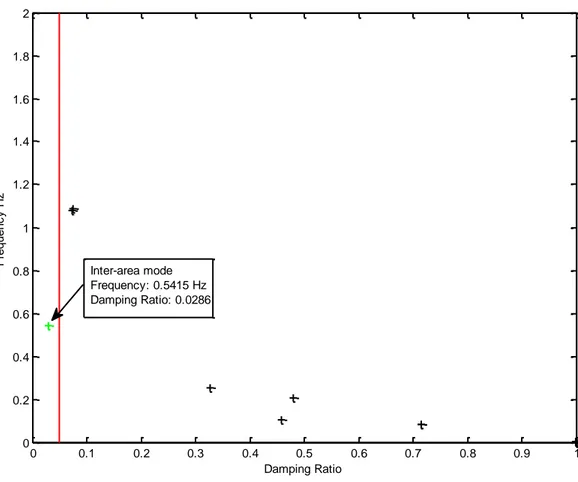
41

Mode Right eigenvalues Damping Frequency Comment

1 0.0000 1.0000 0 Theoritically zero eigenvalues 2 -0.0922 1.0000 0 3 -0.1002 - 0.0000i 1.0000 0.0000 4 -0.1002 + 0.0000i 1.0000 0.0000 5 -0.1003 1.0000 0 6 -0.1844 1.0000 0 7 -0.1845 - 0.0001i 1.0000 0.0000 8 -0.1845 + 0.0001i 1.0000 0.0000 9 -0.1866 1.0000 0 10 -0.1954 1.0000 0 11 -0.1978 1.0000 0 12 -0.1978 1.0000 0 13 -0.5211 - 0.5082i 0.7159 0.0809 14 -0.5211 + 0.5082i 0.7159 0.0809 15 -0.3404 - 0.6595i 0.4587 0.1050 16 -0.3404 + 0.6595i 0.4587 0.1050 17 -0.5320 - 0.5189i 0.7159 0.0826 18 -0.5320 + 0.5189i 0.7159 0.0826 19 -1.1579 1.0000 0 20 -0.7035 - 1.2838i 0.4806 0.2043 21 -0.7035 + 1.2838i 0.4806 0.2043 22 -1.4663 1.0000 0 23 -1.5579 1.0000 0 24 -0.5540 - 1.5977i 0.3276 0.2543 25 -0.5540 + 1.5977i 0.3276 0.2543 26 -1.9050 1.0000 0 27 -1.9894 1.0000 0 28 -1.9906 1.0000 0 29 -2.3663 1.0000 0 30 -2.3837 1.0000 0 31 -3.1146 1.0000 0 32 -3.3944 1.0000 0

33 -0.0974 - 3.4026i 0.0286 0.5415 Lightly-damped inter-area Mode 34 -0.0974 + 3.4026i 0.0286 0.5415 Lightly-damped inter-area Mode 35 -4.6443 1.0000 0 36 -4.6648 1.0000 0 37 -0.4941 - 6.7788i 0.0727 1.0789 38 -0.4941 + 6.7788i 0.0727 1.0789 39 -0.5078 - 6.8357i 0.0741 1.0879 40 -0.5078 + 6.8357i 0.0741 1.0879 41 -10.0712 1.0000 0 42 -10.0718 1.0000 0 43 -10.0992 1.0000 0 44 -10.1102 1.0000 0 45 -19.1942 1.0000 0 46 -19.1961 1.0000 0 47 -19.3047 1.0000 0 48 -19.3924 1.0000 0 49 -20.0000 1.0000 0 50 -20.0000 1.0000 0 51 -20.0000 1.0000 0 52 -20.0000 1.0000 0 53 -28.9774 1.0000 0 54 -30.2323 1.0000 0 55 -33.6969 1.0000 0 56 -34.8376 1.0000 0 57 -36.0189 1.0000 0 58 -36.2034 1.0000 0 59 -37.1492 1.0000 0 60 -37.2206 1.0000 0 61 -50.0001 - 0.0000i 1.0000 0.0000 62 -50.0001 + 0.0000i 1.0000 0.0000 63 -50.0001 1.0000 0 64 -50.0001 1.0000 0

42

There is a lightly damped inter-area mode of with frequency of and damping ratio of . Fig. 4.2 shows the plot of frequency against damping ratio of the system’s modes.

Fig. 4.2 Calculated Modes of IEEE 4-Generator 2-Area Test System

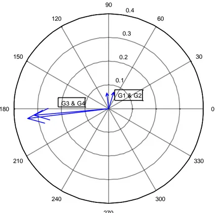
Mode shape and eigenvectors

The eigenvector associated with a mode indicates the relative change in the states which would be observed when the mode of oscillation is excited. Fig. 4.3 shows the compass plot of rotor angle terms of inter-area mode eigenvector. It enables us to confirm that mode 20 is an inter-area mode, since generators 1 and 2 are oscillating against generators 3 and 4. 0 0.1 0.2 0.3 0.4 0.5 0.6 0.7 0.8 0.9 1 0 0.2 0.4 0.6 0.8 1 1.2 1.4 1.6 1.8 2 Damping Ratio F re q u e n c y H z Inter-area mode Frequency: 0.5415 Hz Damping Ratio: 0.0286