Analyzing the persistence of currency substitution using a ratchet variable: the Turkish case

https://www.researchgate.net/publication/5171127

Analyzing the Persistence of

Currency Substitution Using a

Ratchet Variable : The Turkish

Case

14

26

All content following this page was uploaded by Vuslat Us on 05 January 2017. The user has requested enhancement of the downloaded file.

58

Emerging Markets Finance and Trade, vol. 39, no. 4,

July–August 2003, pp. 58–81.

© 2003 M.E. Sharpe, Inc. All rights reserved. ISSN 1540–496X/2003 $9.50 + 0.00.

V

U

Analyzing the Persistence of Currency

Substitution Using a Ratchet Variable

The Turkish Case

Abstract: Although previous studies on currency substitution in Turkey confirm the exist-ence of currency substitution, these works ignore whether this process reached an irrevers-ible stage or not. This paper analyzes the persistence of currency substitution in Turkey through inclusion of a ratchet variable, the past peak value of the currency substitution. Results using an autoregressive distributed lag (ARDL) approach suggest that currency substitution during 1990–93 is not persistent enough to be irreversible. During 1995–99, even though currency substitution in the narrow sense is persistent, currency substitution in the broader sense is not irreversible. Therefore, there is still room for effective monetary policy.

Key words: ARDL approach, cointegration, dollarization, hysteresis, ratchet effect.

Turkish policymakers commonly acknowledged exchange rate as a key policy in-strument that played a crucial role in Turkish stabilization and adjustment pro-grams. Latin American experience also proves that exchange rate policy is the key to the success or failure of such programs. Yet exchange rate issues in Southern Cone countries have been the subject of many researches, but the experience of Turkey has not been sufficiently studied. The aim of this paper is therefore to fill this gap in the literature.

Vuslat Us ([email protected]) is a researcher at the Central Bank of the Republic of Turkey, Research Department, Ankara, and a lecturer at Bilkent University, Department of Economics, Ankara.

Currency substitution, also known as “dollarization,” is when a more stable foreign currency circulates (perhaps illegally) along with the local currency. Al-though, most countries have a domestic currency of their own, without a legal restriction, many governments cannot persuade their citizens to hold only domes-tic currency. Even in the presence of such restrictions, however, foreign currency may substitute domestic currency, because, in today’s global economy, it is im-plausible to assume that no foreign currency is held in the domestic country. Com-panies have strong incentives to diversify their currency holdings in order to facilitate international business. People who make purchases from foreign countries de-mand foreign currency for transactions or people may simply hold currency to diversify their portfolios.

The class of currencies that generally substitutes domestic currencies is restricted to only a few. For example, it would be odd to see international transactions de-nominated in Turkish lira (TL). Yet it is very common to see U.S. dollar-denomi-nated contracts in Turkey or in other countries. Actually, it is estimated that $180

billion or so may be circulating outside the United States.1 _{Sprenkle (1993) notes}

that the Federal Reserve is unable to account for as much as 80 percent of the U.S. dollars held in currency. Why is the U.S. dollar so popular? A currency functions as a medium of exchange, unit of account, and a store of value. The U.S. dollar is popular as a store of value, especially in countries where inflation erodes the value of domestic currency. Due to the same reason, it is commonly used as a unit of account, and so it becomes convenient to use it globally as a medium of exchange. Therefore, today, the U.S. dollar is the most popular vehicle currency—a currency

used by nonresidents in international transactions.2

The earlier works on currency substitution in Turkey provide enough evidence on the existence of currency substitution in Turkey (Akçay et al. 1997; Selçuk 1994, 1997, 2001). Yet we do not have information on whether currency substitu-tion has reached an irreversible stage or not. Then, the quessubstitu-tion is to see whether there is hysteresis in currency substitution in Turkey and model this hysteresis through the inclusion of a ratchet variable. By using alternative measures of cur-rency substitution, the aim of this paper is to find out whether the economy at large has reached a point where currency substitution is costly to be reversed and to decide whether monetary policy may still be effective in altering this trend.

In doing so, this paper will benefit from earlier models that studied hysteresis with the inclusion of a ratchet variable. In economic models that include a ratchet variable, it is assumed that the dependent variable reacts asymmetrically to changes in one of the key explanatory variables. The common practice is to model this ratchet effect through the inclusion of the past peak value of an independent vari-able in addition to the current value of that varivari-able or of the past peak value of one

of the dependent variables.3 _{The existence of an asymmetry in currency}

substitu-tion is attributed to the fixed costs of developing, learning, and applying new money management techniques to beat inflation. Once these fixed costs are paid for, there are a few incentives to switch back to domestic currency, thus causing a ratchet

effect on the demand for domestic and foreign currency, even if macroeconomic

stabilization is achieved.4

The credibility of the policymakers in these stabilization programs may shorten or prolong the duration of the ratchet effect as well as its influence. Only a signifi-cant decline in inflation or a considerable appreciation of the currency can over-come the sunk cost of finding strategies to beat inflation and provide enough incentives to revert back to traditional domestic money balances. Information about the degree at which the currency substitution is irreversible is very crucial in order to implement an effective monetary policy.

Some Stylized Facts About the Turkish Economy

This section gives a brief account of the Turkish economy with particular empha-sis on the recent decade. Over the past few years, large financing requirement of the government, including not only the central government but also the extra-budgetary funds, the local authorities, the social security institutions, and the fi-nancial and nonfifi-nancial state economic enterprises, would have resulted in an exploding ratio of debt to gross domestic product (GDP) were it not for the mon-etization of these deficits through increasingly higher inflation rates. Large budget deficits are in turn the result of both substantially negative budget balances and high and rising real interest rates. In a chronic inflationary environment deprived of a monetary anchor, high real interest rates become, in fact, both the cause and the consequence of high inflation. That is, they feed into high inflation and in turn are fed by high inflation and the associated risks. Yet chronic and high inflation has not degenerated into hyperinflation as it did in most other countries. This is to be credited to the very slow pace at which inflation has eroded the demand for base money—a trait unique to Turkey.

The Turkish economy has experienced economic crises since the 1990s. Exter-nal factors have played important roles in these crises. Yet the main reasons for the crises are the unsustainable domestic debt dynamics and the lack of structural reforms, especially in the financial sector. More specifically, the ratio of public sector debt to gross national product (GNP) has increased from 29 percent in 1990 to 61 percent at the end of 1999. The ratio of domestic borrowing to GNP rose up to 42 percent by the end of 1999, from 6 percent in 1990. In addition to high public deficits, in the post-1994 period, public sector has been net external debt payer, and this put pressure on the real interest rates due to insufficient financial sector deepening.

The instability in the financial sector combined with high and variable inflation rate caused the credibility of the TL to drop. During 1990–99, the substitution of the TL by foreign exchange accelerated. The share of foreign exchange deposits and reverse repo accounts in the overall deposits increased from 25 percent in 1990 to 42 percent in 1999. Moreover, the foreign exchange-denominated liabili-ties of the banks have increased disproportionately due to attractiveness of returns

on TL-denominated securities; this put even more pressure on the open position of the banks, causing banks to expose more risk and vulnerability to exchange rate changes. Under these circumstances, therefore, it is critical to know the degree of persistence of the currency substitution in order to find an efficient monetary policy rule in order to reverse it.

Econometric Methodology

After these stylized facts on the Turkish economy, this section outlines the empiri-cal currency substitution model that captures the ratchet effect. The econometric model adopted in this study lies on a simple structural model based on a standard money demand function that incorporates interest rate differential and deprecia-tion. Following Mongardini and Mueller (1999, 2000), the currency substitution model is

t t L t L t L t t

CS = α +CS− −1 + β1IntDiff− + β2Exch− + β3Ratchet +u, (1)

where CS is a measure of currency substitution; IntDiff is the interest rate differen-tial between domestic and foreign assets; Exch is the depreciation of the TL; Ratchet is the variable that denotes the persistence effect in the currency substitution; and

ut is the error term. Description of the Data

After the introduction on the empirical model in the previous part, this section will provide detailed information about the data set and the next section will present the results of the empirical analysis of this paper. The data that are used are pub-licly available from the data set of the Central Bank of the Republic of Turkey

(CBRT).5 _{The data set covers the periods from 1990 to 1993 and from 1995 to}

1999. The frequency of the data is monthly.

The notation that is adopted is as follows: CS is a measure of currency substitu-tion; IntDiff is the interest rate differential between TL-denominated time deposits

and foreign exchange-denominated time deposits.6 _{Exch is the differenced logged}

nominal depreciation of the TL against the basket exchange rate, which is

com-posed of $1 + 1.5 DM.7 _{IntDiff1 measures the differential between TL-denominated}

one-month time deposits and foreign exchange-denominated one-month time de-posits. The returns on one-month foreign exchange deposits is a weighted average of the return on U.S. dollar-denominated deposits and German mark-denominated deposits, where weights are assigned in proportion to the weights of the U.S. dollar and German mark in the basket exchange rate. The interest rates are nominal.

In order to see whether the ratchet effect becomes more significant or not as one goes from narrow to broader definitions of currency substitution, CS has alterna-tive sets of definitions. More specifically, CS is defined as the logarithm of foreign exchange-denominated deposits/M1 in the narrow sense, or foreign

exchange-de-nominated deposits/total deposits in the broad sense. Then, apparently, CS1 is for-eign exchange-denominated deposits/M1 and CSd is forfor-eign

exchange-denomi-nated deposits/total deposits.8 _{The ratchet variable is denoted by R1, the past peak}

value of the CS1, or, correspondingly, Rd, the past peak value of the CSd. All the

series are seasonally adjusted.9

The period of analysis starts from 1990 and ends in 1999. However, the crisis year of 1994 is commented out in order to be able to compare the precrisis and postcrisis periods in terms of the degree of persistence of currency substitution, and in order to find out at which level of monetary aggregation this persistence is more apparent. Also, the year 2000 and onward is excluded because the CBRT started to implement the disinflation program as of the beginning of the year 2000. However, the program was halted as result of the financial crises in November 2000 and in February 2001. So, adequate data for the analysis of currency substi-tution after the implementation of the disinflation program do not exist. Therefore, this paper analyzes two subperiods, where the first one covers the period from 1990 to 1993 and the second period is from 1995 to 1999.

The ARDL Approach to Cointegration

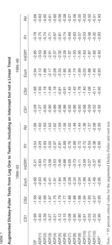
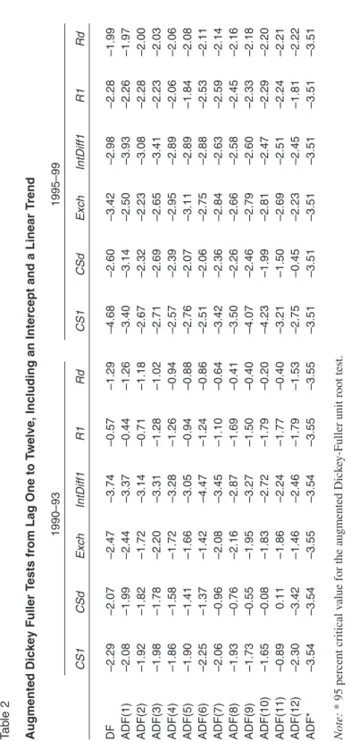
Before starting the econometric procedure, this section will proceed by testing the stationarity properties of the series. Tables 1 and 2 show the results of the aug-mented Dickey-Fuller unit root tests for each series described above. The tables indicate that all series are nonstationary. Following Mongardini and Mueller (1999, 2000), a good approach is to apply the autoregressive distributed lag procedure as outlined by Pesaran and Shin (1995). This approach analyzes the long-run rela-tions when the underlying variables are integrated of order one.

According to Pesaran and Shin (1995), using this approach after appropriate augmentation of the order of the ARDL (autoregressive distributed lag) model, the ordinary least squares (OLS) estimators of the short-run parameters are consistent with the asymptotically singular covariance matrix. The ARDL-based estimators of the run coefficients are super-consistent, and valid inferences on the

long-run parameters can be made using standard normal asymptotic theory.10

The authors also analyze the relationship between the ARDL procedure and the fully modified OLS approach of Phillips and Hansen, for the estimation of cointegrating relations. They also compare the small sample performance of these two approaches via Monte Carlo experiments. These results provide strong evi-dence in favor of the traditional ARDL approach. This approach also has the addi-tional advantage of producing consistent estimates of the long-run coefficients that are asymptotically normal regardless of whether the underlying independent variables are integrated or order one or zero.

T

a

b

le 1

Augmented Dickey-Fuller T

ests from Lag One to T

welve, Including an Intercept but not a Linear T

rend 1990–93 1995–99 C S 1 C S d Exch IntDiff1 R 1 R d C S 1 C S d Exch IntDiff1 R 1 R d D F –2.99 –1.58 –2.66 –5.21 –3.54 –1.66 –2.09 –1.68 –2.94 –2.85 –0.78 –0.66 ADF(1) –3.40 –1.60 –2.63 –3.83 –3.25 –1.63 –1.27 –1.93 –2.12 –3.53 –0.75 –0.63 ADF(2) –3.39 –1.68 –1.95 –3.73 –2.93 –1.63 –0.93 –1.18 –1.88 –2.66 –0.74 –0.62 ADF(3) –3.27 –1.67 –2.41 –3.58 –3.02 –1.63 –0.90 –1.49 –2.17 –2.91 –0.71 –0.61 ADF(4) –3.21 –1.75 –1.91 –3.53 –2.97 –1.62 –0.89 –1.18 –2.28 –2.37 –0.67 –0.60 ADF(5) –3.12 –1.79 –1.84 –3.46 –2.81 –1.59 –0.88 –0.81 –2.33 –2.32 –0.61 –0.59 ADF(6) –3.15 –1.77 –1.58 –4.88 –2.89 –1.56 –0.86 –0.91 –1.95 –2.26 –0.74 –0.58 ADF(7) –3.08 –1.86 –2.28 –4.00 –2.76 –1.52 –0.92 –1.45 –1.94 –1.97 –0.69 –0.57 ADF(8) –2.95 –1.88 –2.34 –3.73 –2.98 –1.48 –0.86 –1.42 –1.74 –1.93 –0.63 –0.56 ADF(9) –2.80 –1.88 –2.04 –4.11 –2.72 –1.44 –0.83 –1.78 –1.99 –1.95 –0.57 –0.55 ADF(10) –2.61 –1.94 –1.89 –3.59 –2.72 –1.36 –0.68 –1.40 –2.03 –1.83 –0.53 –0.53 ADF(11) –2.03 –1.93 –1.94 –3.27 –2.53 –1.37 –0.59 –1.06 –1.88 –1.87 –0.48 –0.52 ADF(12) –2.52 –2.57 –1.46 –3.37 –2.38 –2.08 –0.52 –0.11 –1.40 –1.82 –0.32 –0.51 ADF* –2.95 –2.95 –2.95 –2.95 –2.95 –2.95 –2.92 –2.92 –2.93 –2.92 –2.93 –2.93 Note: * 95 percent critical v alue f

or the augmented Dick

T

a

b

le 2

Augmented Dickey Fuller T

ests from Lag One to T

welve, Including an Intercept and a Linear T

rend 1990–93 1995–99 C S 1 C S d Exch IntDiff1 R 1 R d C S 1 C S d Exch IntDiff1 R 1 R d D F –2.29 –2.07 –2.47 –3.74 –0.57 –1.29 –4.68 –2.60 –3.42 –2.98 –2.28 –1.99 ADF(1) –2.08 –1.99 –2.44 –3.37 –0.44 –1.26 –3.40 –3.14 –2.50 –3.93 –2.26 –1.97 ADF(2) –1.92 –1.82 –1.72 –3.14 –0.71 –1.18 –2.67 –2.32 –2.23 –3.08 –2.28 –2.00 ADF(3) –1.98 –1.78 –2.20 –3.31 –1.28 –1.02 –2.71 –2.69 –2.65 –3.41 –2.23 –2.03 ADF(4) –1.86 –1.58 –1.72 –3.28 –1.26 –0.94 –2.57 –2.39 –2.95 –2.89 –2.06 –2.06 ADF(5) –1.90 –1.41 –1.66 –3.05 –0.94 –0.88 –2.76 –2.07 –3.11 –2.89 –1.84 –2.08 ADF(6) –2.25 –1.37 –1.42 –4.47 –1.24 –0.86 –2.51 –2.06 –2.75 –2.88 –2.53 –2.11 ADF(7) –2.06 –0.96 –2.08 –3.45 –1.10 –0.64 –3.42 –2.36 –2.84 –2.63 –2.59 –2.14 ADF(8) –1.93 –0.76 –2.16 –2.87 –1.69 –0.41 –3.50 –2.26 –2.66 –2.58 –2.45 –2.16 ADF(9) –1.73 –0.55 –1.95 –3.27 –1.50 –0.40 –4.07 –2.46 –2.79 –2.60 –2.33 –2.18 ADF(10) –1.65 –0.08 –1.83 –2.72 –1.79 –0.20 –4.23 –1.99 –2.81 –2.47 –2.29 –2.20 ADF(11) –0.89 0.11 –1.86 –2.24 –1.77 –0.40 –3.21 –1.50 –2.69 –2.51 –2.24 –2.21 ADF(12) –2.30 –3.42 –1.46 –2.46 –1.79 –1.53 –2.75 –0.45 –2.23 –2.45 –1.81 –2.22 ADF* –3.54 –3.54 –3.55 –3.54 –3.55 –3.55 –3.51 –3.51 –3.51 –3.51 –3.51 –3.51 Note: * 95 percent critical v alue f

or the augmented Dick

The Estimation Results

After this brief overview on the ARDL approach in the previous part, this section will proceed by testing the persistence of currency substitution under alternative measures. Using the ARDL approach outlined above, the analysis starts by first including the ratchet variable and then, in the next step, this variable is excluded. For each definition of currency substitution, the error correction term (ecm) is found according to Equation (1). More specifically, the lagged error term from the regression of CS on the right-hand-side terms in Equation (1) is plugged into the Equation (2), and where L, the lag number, is set according to the Akaike Informa-tion Criterion (AIC), such that:

t t L t L t L t L t

CS CS− −1 1 intdiff− 2Exch− 3 Ratchet− ecm−1.

∆ = ∆α + ∆ + β ∆ + β + β ∆ + (2)

Again, the optimal lag length for each variable is determined according to the AIC. The estimation of the Equation (1) gives us the “static” foreign money de-mand, whereas, the estimation of Equation (2), when the variables are in differ-ences, and with the inclusion of the lagged error term, is a dynamic version of the static foreign money demand.

The parameter estimate of this lagged error term provides information about the adjustment speed of foreign money toward equilibrium. The reason to distin-guish between static and dynamic foreign money demand function is important since this method allows us to differentiate between the short-term and long-term behavior of foreign money demand. This distinction is crucial given that Turkey is

out of the equilibrium phase.11

The Results of the Analysis Using CS1 as the Ratchet Variable

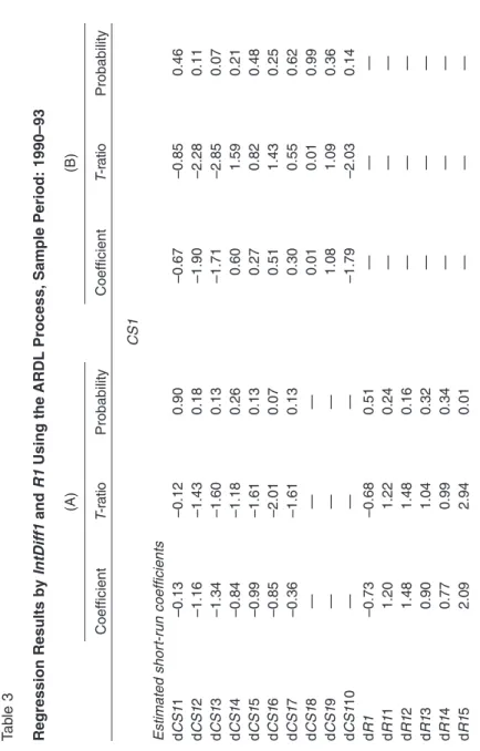
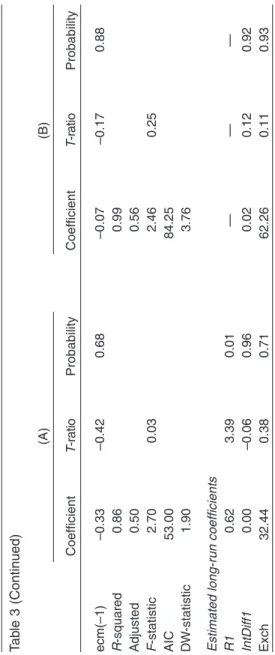
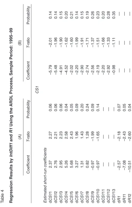
Using CS1 as the measure of the currency substitution, the regression produces mostly insignificant short-run coefficients with the inclusion of the ratchet vari-able. By the exclusion of the ratchet variable, most of the short-run coefficients are insignificant including the error correction term. With the inclusion of the ratchet variable, the only significant long-run coefficient turns out to be the ratchet vari-able with a positive sign. This indicates that as the past peak value of CS1 in-creases, the current CS1 increases in the long run. The exclusion of the ratchet variable on the other hand produces insignificant long-run coefficients (Table 3). In the second period, 1995–99, using CS1 as the dependent variable, the regres-sion results show that including the ratchet variable produces mostly significant short-run coefficients. However, the coefficient of the change in the depreciation rate of the TL against the basket is of the wrong sign. The short-run coefficient of the change in IntDiff1 is significant, however, mostly with a positive sign. This indicates that as the gap between the rates on TL-denominated one-month time deposits and the foreign exchange-denominated one-month time deposits increased, demand for foreign exchange increased. Normally, we would have expected this

T a b le 3 Regression Results by IntDiff1 and R1 Using the ARDL

Process, Sample Period: 1990–93

(A) (B) Coefficient T -r atio Probability Coefficient T -r atio Probability CS1 Estimated shor t-r un coefficients d CS1 1 –0.13 –0.12 0.90 –0.67 –0.85 0.46 d CS1 2 –1.16 –1.43 0.18 –1.90 –2.28 0.11 d CS1 3 –1.34 –1.60 0.13 –1.71 –2.85 0.07 d CS1 4 –0.84 –1.18 0.26 0.60 1.59 0.21 d CS1 5 –0.99 –1.61 0.13 0.27 0.82 0.48 d CS1 6 –0.85 –2.01 0.07 0.51 1.43 0.25 d CS1 7 –0.36 –1.61 0.13 0.30 0.55 0.62 d CS1 8 — — — 0.01 0.01 0.99 d CS1 9 — — — 1.08 1.09 0.36 d CS1 1 0 — — — –1.79 –2.03 0.14 d R1 –0.73 –0.68 0.51 — — — d R1 1 1.20 1.22 0.24 — — — d R1 2 1.48 1.48 0.16 — — — d R1 3 0.90 1.04 0.32 — — — d R1 4 0.77 0.99 0.34 — — — d R1 5 2.09 2.94 0.01 — — —

d IntDiff1 0.02 1.28 0.22 0.03 0.76 0.50 d IntDiff1 1 –0.01 –0.30 0.77 –0.05 –1.43 0.25 d IntDiff1 2 0.00 0.05 0.96 0.03 1.42 0.25 d IntDiff1 3 0.02 1.89 0.08 0.03 1.53 0.22 d IntDiff1 4 –0.01 –0.93 0.37 0.02 0.88 0.44 d IntDiff1 5 0.01 1.33 0.20 0.02 0.88 0.44 d IntDiff1 6 –0.01 –1.10 0.29 –0.01 –0.51 0.64 d IntDiff1 7 — — — –0.01 –0.39 0.72 d IntDiff1 8 — — — 0.06 1.42 0.25 d IntDiff1 9 — — — –0.06 –1.56 0.22 d IntDiff1 1 0 — — — 0.09 2.69 0.08 d Exch 2.59 0.78 0.45 2.92 0.85 0.46 d Exch 1 –9.52 –3.25 0.01 –3.72 –0.28 0.80 d Exch 2 0.85 0.33 0.75 6.31 0.58 0.60 d Exch 3 –6.45 –2.56 0.02 9.13 0.64 0.57 d Exch 4 — — — –4.97 –0.43 0.70 d Exch 5 — — — 9.14 0.62 0.58 d Exch 6 — — — –13.35 –1.25 0.30 d Exch 7 — — — 11.67 1.03 0.38 d Exch 8 — — — –11.13 –1.33 0.28 d Exch 9 — — — –5.45 –0.93 0.42 d Exch 1 0 — — — –11.92 –2.53 0.09 (continues)

T a b le 3 (Continued) (A) (B) Coefficient T -r atio Probability Coefficient T -r atio Probability ecm(–1) –0.33 –0.42 0.68 –0.07 –0.17 0.88 R -squared 0.86 0.99 Adjusted 0.50 0.56 F -statistic 2.70 0.03 2.46 0.25 AIC 53.00 84.25 D W -statistic 1.90 3.76 Estimated long-r un coefficients R1 0.62 3.39 0.01 — — — IntDiff1 0.00 –0.06 0.96 0.02 0.12 0.92 Exch 32.44 0.38 0.71 62.26 0.11 0.93

relationship to be negative. However, this positive relationship between interest rate differential and the demand for foreign exchange suggests that the high level-ing of the interest rate and its further increase shifted the domestic portfolio allo-cations toward foreign-denominated assets even more due to the increase in risk premium. Therefore, we see a positive relationship between the interest rate differ-ential and the demand for foreign exchange in the short run. However, in the long run, with or without the ratchet variable, we see a negative relationship between the interest rate differential and the demand for foreign exchange, that is, as the return on TL-denominated assets increase, people switch from foreign exchange-denominated assets to TL-exchange-denominated assets.

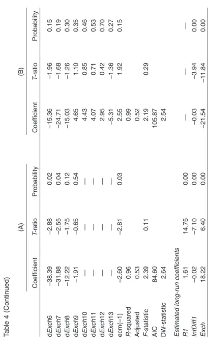
In the second period, with the inclusion of the ratchet variable, all the long-run coefficients turn out to be both significant and of the correct sign. The exclusion of the ratchet variable, on the other hand, produces significant long-run coefficients with the interest rate differential having a positive sign. The inclusion of the ratchet variable produces a higher semi-elasticity of the demand for foreign exchange with respect to interest rate. On the other hand, without the ratchet variable, the elasticity of the demand for foreign exchange with respect to the depreciation rate gets higher (Table 4).

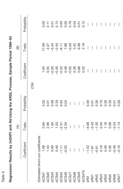
The Results of the Analysis Using CSd as the Ratchet Variable

CSd as the measure of currency substitution produces significant short-run

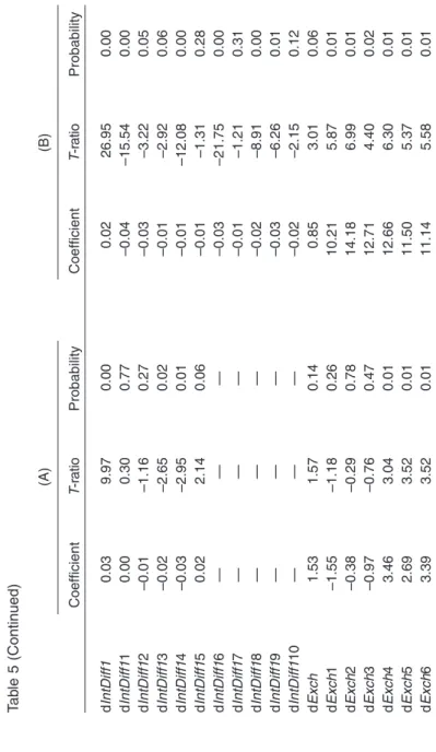
coeffi-cients with or without the ratchet variable in the first period, 1990–93. By exclud-ing the ratchet variable, the significance of the change in the depreciation rate and the interest rate differential increases. However, the long-run estimates of the coef-ficients with the exclusion of the ratchet variable are of the wrong sign, though they are significant. The long-run estimation of the coefficients with the inclusion of the ratchet variable produces an insignificant depreciation rate coefficient. How-ever, the long-run coefficient of the ratchet variable is significant (Table 5).

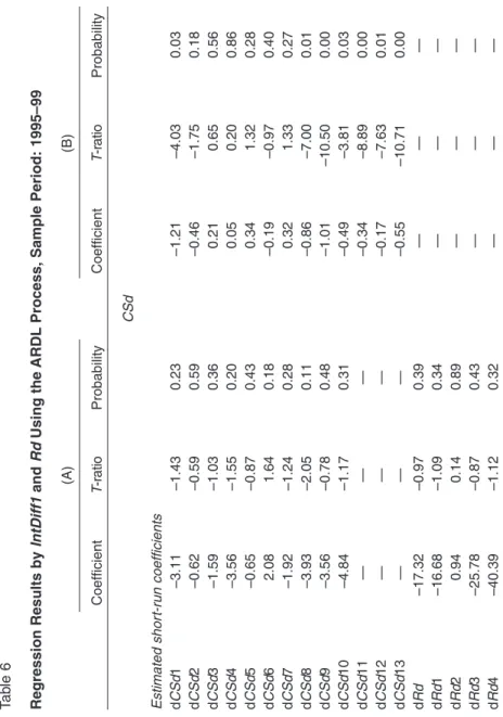
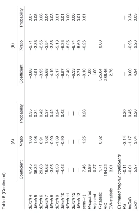
In the second period, from 1995 to 1999, CSd as the measure of currency substi-tution produces mostly insignificant coefficients in the short run with the inclusion of the ratchet variable. The exclusion of the ratchet variable, on the other hand, produces significant short-run coefficients of the correct sign. The long-run esti-mates of the coefficients, without the ratchet variable, produce only a significant coefficient for depreciation rate. Both the depreciation rate and the ratchet variable turn out to be significant with the inclusion of the ratchet variable (Table 6).

Concluding Remarks

This paper analyzes the persistence in currency substitution at different levels, in two subperiods: 1990–93 and 1995–99. In doing so, a ratchet variable—the past peak value of the currency substitution measure—is included into the analysis. The regression results show that, in the first period, for both levels of currency

T a b le 4 Regression Results by IntDiff1 and R1 Using the ARDL

Process, Sample Period: 1995–99

(A) (B) Coefficient T -r atio Probability Coefficient T -r atio Probability CS1 Estimated shor t-r un coefficients d CS1 1 2.37 2.27 0.06 –5.79 –2.01 0.14 d CS1 2 2.76 2.21 0.06 –5.48 –1.96 0.14 d CS1 3 2.95 2.23 0.06 –4.91 –1.90 0.15 d CS1 4 5.26 2.58 0.04 –4.52 –1.62 0.20 d CS1 5 5.68 2.43 0.05 –2.02 –1.60 0.21 d CS1 6 3.27 1.96 0.09 –2.20 –1.99 0.14 d CS1 7 1.31 1.43 0.20 –2.90 –1.91 0.15 d CS1 8 0.82 1.28 0.24 –2.74 –1.71 0.19 d CS1 9 –0.97 –1.99 0.09 –2.56 –1.37 0.26 d CS1 1 0 –0.97 –1.65 0.14 –2.19 –1.51 0.23 d CS1 1 1 — — — –2.20 –1.66 0.20 d CS1 1 2 — — — –2.92 –1.33 0.28 d CS1 1 3 — — — –0.98 –1.11 0.35 d R1 –2.57 –2.18 0.07 — — — d R1 1 –7.08 –2.43 0.05 — — — d R1 2 –10.51 –2.60 0.04 — — —

d R1 3 –15.99 –2.72 0.03 — — — d R1 4 –14.49 –2.51 0.04 — — — d R1 5 –6.37 –1.82 0.11 — — — d R1 6 –4.08 –1.79 0.12 — — — d R1 7 –9.10 –2.76 0.03 — — — d R1 8 –4.66 –2.11 0.07 — — — d IntDiff1 –0.01 –1.04 0.33 0.02 2.09 0.13 d IntDiff1 1 0.10 2.64 0.03 –0.05 –1.20 0.32 d IntDiff1 2 0.08 2.56 0.04 –0.04 –2.41 0.10 d IntDiff1 3 0.05 2.34 0.05 –0.08 –1.63 0.20 d IntDiff1 4 –0.01 –0.58 0.58 –0.04 –1.30 0.28 d IntDiff1 5 0.03 2.19 0.07 –0.02 –1.29 0.29 d IntDiff1 6 0.03 1.83 0.11 –0.02 –0.98 0.40 d IntDiff1 7 0.04 2.83 0.03 –0.02 –0.81 0.48 d IntDiff1 8 0.03 1.61 0.15 0.02 1.15 0.33 d IntDiff1 9 0.01 1.16 0.28 0.01 0.55 0.62 d IntDiff1 1 0 0.04 2.16 0.07 –0.01 –0.74 0.51 d IntDiff1 1 1 — — — 0.01 0.52 0.64 d IntDiff1 1 2 — — — 0.00 –0.26 0.81 d IntDiff1 1 3 — — — –0.02 –1.20 0.32 d Exch –23.20 –2.47 0.04 18.89 2.31 0.10 d Exch 1 –85.64 –2.73 0.03 –27.20 –1.93 0.15 d Exch 2 –64.41 –2.41 0.05 –27.54 –1.61 0.21 d Exch 3 –43.44 –2.26 0.06 –20.98 –1.21 0.31 d Exch 4 –49.35 –2.70 0.03 –12.79 –1.23 0.31 d Exch 5 –41.36 –2.56 0.04 –26.16 –1.63 0.20 (continues)

T a b le 4 (Continued) (A) (B) Coefficient T -r atio Probability Coefficient T -r atio Probability d Exch 6 –38.39 –2.88 0.02 –15.36 –1.96 0.15 d Exch 7 –31.88 –2.55 0.04 –24.71 –1.68 0.19 d Exch 8 –12.22 –1.75 0.12 –15.03 –1.26 0.30 d Exch 9 –1.91 –0.65 0.54 4.65 1.10 0.35 d Exch 1 0 — — — 4.43 0.85 0.46 d Exch 1 1 — — — 4.07 0.71 0.53 d Exch 1 2 — — — 2.95 0.42 0.70 d Exch 1 3 — — — –5.31 –1.36 0.27 ecm(–1) –2.60 –2.81 0.03 2.55 1.92 0.15 R -squared 0.96 0.99 Adjusted 0.53 0.52 F -statistic 2.39 0.11 2.19 0.29 AIC 84.60 105.87 D W -statistic 2.64 2.54 Estimated long-r un coefficients R1 1.61 14.75 0.00 — — — IntDiff1 –0.02 –7.10 0.00 –0.03 –3.94 0.00 Exch 18.22 6.40 0.00 –21.54 –11.84 0.00

T a b le 5 Regression Results by IntDiff1 and Rd Using the ARDL

Process, Sample Period 1990–93

(A) (B) Coefficient T -r atio Probability Coefficient T -r atio Probability CSd Estimated shor t-r un coefficients d CS d 1 1.08 2.84 0.02 1.04 17.06 0.00 d CS d 2 1.43 2.99 0.01 0.55 2.27 0.11 d CS d 3 0.99 1.94 0.08 –0.30 –5.44 0.01 d CS d 4 0.49 1.03 0.33 –0.30 –2.04 0.13 d CS d 5 –1.11 –2.31 0.04 –0.33 –8.11 0.00 d CS d 6 –0.55 –2.34 0.04 0.48 7.88 0.00 d CS d 7 — — — –0.05 –0.29 0.79 d CS d 8 — — — 0.28 3.42 0.04 d CS d 9 — — — 0.88 6.08 0.01 d CS d 1 0 — — — 0.52 2.18 0.12 d Rd –1.52 –4.08 0.00 — — — d Rd 1 –1.81 –3.43 0.01 — — — d Rd 2 –0.61 –1.20 0.26 — — — d Rd 3 0.16 0.40 0.70 — — — d Rd 4 0.46 1.18 0.26 — — — d Rd 5 0.30 0.99 0.35 — — — d Rd 6 –0.49 –3.24 0.01 — — — d Rd 7 –0.16 –1.14 0.28 — — — (continues)

T a b le 5 (Continued) (A) (B) Coefficient T -r atio Probability Coefficient T -r atio Probability d IntDiff1 0.03 9.97 0.00 0.02 26.95 0.00 d IntDiff1 1 0.00 0.30 0.77 –0.04 –15.54 0.00 d IntDiff1 2 –0.01 –1.16 0.27 –0.03 –3.22 0.05 d IntDiff1 3 –0.02 –2.65 0.02 –0.01 –2.92 0.06 d IntDiff1 4 –0.03 –2.95 0.01 –0.01 –12.08 0.00 d IntDiff1 5 0.02 2.14 0.06 –0.01 –1.31 0.28 d IntDiff1 6 — — — –0.03 –21.75 0.00 d IntDiff1 7 — — — –0.01 –1.21 0.31 d IntDiff1 8 — — — –0.02 –8.91 0.00 d IntDiff1 9 — — — –0.03 –6.26 0.01 d IntDiff1 1 0 — — — –0.02 –2.15 0.12 d Exch 1.53 1.57 0.14 0.85 3.01 0.06 d Exch 1 –1.55 –1.18 0.26 10.21 5.87 0.01 d Exch 2 –0.38 –0.29 0.78 14.18 6.99 0.01 d Exch 3 –0.97 –0.76 0.47 12.71 4.40 0.02 d Exch 4 3.46 3.04 0.01 12.66 6.30 0.01 d Exch 5 2.69 3.52 0.01 11.50 5.37 0.01 d Exch 6 3.39 3.52 0.01 11.14 5.58 0.01

d Exch 7 — — — 6.73 3.92 0.03 d Exch 8 — — — 6.10 7.37 0.01 d Exch 9 — — — 3.03 3.18 0.05 d Exch 1 0 — — — 1.46 4.75 0.02 ecm(-1) –0.65 –1.98 0.07 –1.82 –5.11 0.01 R -squared 0.96 1.00 Adjusted 0.80 1.00 F -statistic 6.76 0.00 208.98 0.00 AIC 96.20 182.65 D W -statistic 2.62 3.76 Estimated long-r un coefficients Rd 0.50 3.55 0.01 — — — IntDiff1 0.02 2.75 0.03 0.03 128.63 0.01 Exch –0.74 –0.35 0.74 –4.70 –15.33 0.04

T a b le 6 Regression Results by IntDiff1 and Rd Using the ARDL

Process, Sample Period: 1995–99

(A) (B) Coefficient T -r atio Probability Coefficient T -r atio Probability CSd Estimated shor t-r un coefficients d CSd 1 –3.11 –1.43 0.23 –1.21 –4.03 0.03 d CSd 2 –0.62 –0.59 0.59 –0.46 –1.75 0.18 d CSd 3 –1.59 –1.03 0.36 0.21 0.65 0.56 d CSd 4 –3.56 –1.55 0.20 0.05 0.20 0.86 d CSd 5 –0.65 –0.87 0.43 0.34 1.32 0.28 d CSd 6 2.08 1.64 0.18 –0.19 –0.97 0.40 d CSd 7 –1.92 –1.24 0.28 0.32 1.33 0.27 d CSd 8 –3.93 –2.05 0.11 –0.86 –7.00 0.01 d CSd 9 –3.56 –0.78 0.48 –1.01 –10.50 0.00 d CSd 1 0 –4.84 –1.17 0.31 –0.49 –3.81 0.03 d CSd 1 1 — — — –0.34 –8.89 0.00 d CSd 1 2 — — — –0.17 –7.63 0.01 d CSd 1 3 — — — –0.55 –10.71 0.00 d Rd –17.32 –0.97 0.39 — — — d Rd 1 –16.68 –1.09 0.34 — — — d Rd 2 0.94 0.14 0.89 — — — d Rd 3 –25.78 –0.87 0.43 — — — d Rd 4 –40.39 –1.12 0.32 — — —

d Rd 5 –42.85 –1.01 0.37 — — — d Rd 6 –22.78 –0.91 0.41 — — — d Rd 7 –25.80 –0.72 0.51 — — — d Rd 8 –39.24 –1.13 0.32 — — — d Rd 9 –6.18 –0.42 0.70 — — — d Rd 1 0 –10.92 –0.45 0.67 — — — d IntDiff1 0.01 0.49 0.65 0.00 3.92 0.03 d IntDiff1 1 –0.10 –0.86 0.44 0.02 34.66 0.00 d IntDiff1 2 –0.09 –1.01 0.37 0.01 21.45 0.00 d IntDiff1 3 –0.07 –0.72 0.51 0.01 13.33 0.00 d IntDiff1 4 –0.02 –0.76 0.49 0.02 19.92 0.00 d IntDiff1 5 0.00 –0.18 0.87 0.01 15.42 0.00 d IntDiff1 6 0.01 0.84 0.45 0.02 14.93 0.00 d IntDiff1 7 0.06 1.57 0.19 0.01 32.83 0.00 d IntDiff1 8 0.05 1.64 0.18 0.02 18.63 0.00 d IntDiff1 9 0.06 0.78 0.48 0.02 17.22 0.00 d IntDiff1 1 0 0.03 1.39 0.24 0.01 14.15 0.00 d IntDiff1 1 1 — — — 0.01 21.58 0.00 d IntDiff1 1 2 — — — 0.01 13.96 0.00 d IntDiff1 1 3 — — — 0.01 13.23 0.00 d Exch 17.94 0.96 0.39 2.95 28.76 0.00 d Exch 1 68.78 1.06 0.35 –7.79 –5.29 0.01 d Exch 2 61.70 1.01 0.37 –5.90 –4.74 0.02 d Exch 3 50.41 1.02 0.37 –5.69 –3.95 0.03 (continues)

T a b le 6 (Continued) (A) (B) Coefficient T -r atio Probability Coefficient T -r atio Probability d Exch 4 47.45 1.06 0.35 –3.88 –2.71 0.07 d Exch 5 36.32 1.08 0.34 –4.91 –3.33 0.05 d Exch 6 29.88 0.91 0.42 –3.95 –2.55 0.08 d Exch 7 16.62 1.02 0.37 –5.68 –3.54 0.04 d Exch 8 –3.05 –0.90 0.42 –4.19 –3.86 0.03 d Exch 9 –8.30 –1.39 0.24 –5.17 –5.13 0.01 d Exch 10 –4.42 –0.90 0.42 –6.57 –6.33 0.01 d Exch 11 — — — –7.40 –8.25 0.00 d Exch 12 — — — –6.33 –8.74 0.00 d Exch 13 — — — –2.71 –5.60 0.01 ecm(–1) 7.46 1.25 0.28 –0.10 –0.26 0.81 R -squared 0.99 1.00 Adjusted 0.37 1.00 F -statistic 1.71 0.32 525.64 0.00 AIC 164.22 286.46 D W -statistic 3.01 2.76 Estimated long-r un coefficients Rd –0.11 –3.14 0.20 — — — IntDiff1 –0.01 –1.17 0.45 0.00 –0.96 0.34 Exch 5.97 3.04 0.20 4.94 2.20 0.03

substitution, the inclusion of the ratchet variable into the model produces insig-nificant coefficients. Therefore, this result suggests that in the first period, cur-rency substitution is not persistent enough to be irreversible. However, in the second period, currency substitution in the narrow sense produces significant coefficients for the ratchet variable. Yet the same conclusion cannot be reached for the cur-rency substitution in the broader sense. Therefore, in the second period, the ratio of foreign-denominated deposits to M1 has become persistent. On the other hand, currency substitution in the broad sense is still not persistent, given the mostly insignificant coefficients produced with the inclusion of the ratchet variable into the model.

The empirical evidence and econometric results show that although there may be a ratchet effect in the narrow sense currency substitution, this effect is not de-tectable in the overall economy, that is, the portfolio allocation preferences of domestic residents are not persistent. The monetary authorities can therefore con-duct effective policies to induce reversal in the narrow sense of currency substitu-tion. Nevertheless, one should be careful about the implications of these results. The conclusion about currency substitution not being subject to a ratchet effect should not be misleading, as these results are based on figures of foreign currency deposits. Clearly, the currency substitution measure should also include foreign currency in circulation. However, such data are not available. Therefore, this study is incomplete. Yet the scope of this paper is not finding such data or a proxy. Therefore, for further research, one should find a more accurate measure of cur-rency substitution, and repeat this exercise using this new measure. Only then can one conclude whether there is room for monetary policy to be effective or not.

Notes

1. This figure is taken from Rivera-Batiz and Rivera-Batiz (1994, p. 71). 2. This definition is borrowed from Krugman (1980).

3. See the previous models that include the ratchet variable by Enzler et al. (1976), Quick and Paulus (1979), Simpson and Porter (1980), Piterman (1988), Kamin and Ericsson (1993), and Duesenbery (1952).

4. See Dornbusch and Reynoso (1989), Dornbusch et al. (1990), Sturzenegger (1992), and Guidotti and Rodriguez (1991).

5. CBRT provides general statistics through the electronic data delivery system (EDDS). For more information, visit tcmbf40.tcmb.gov.tr/cbt.html.

6. Mongardini and Mueller (1999, 2000) take the difference between the average monthly yield on three-month Kyrgyz T-bills and the average monthly yield on three-month U.S. T-bills. However, this differential, rather than measuring the degree of sensitivity of cur-rency substitution with respect to interest rate differential, measures the degree of sensitiv-ity of asset substitution with respect to the interest rate differential. Therefore, in this study, the difference between the domestic interest rate on TL-denominated time deposits and domestic interest rate on foreign exchange-denominated time deposits is taken as the inter-est rate differential.

7. Forty percent of Turkey’s international trade is U.S. dollar-denominated and the rest is German mark-denominated. Therefore, this basket exchange rate is a simplified trade-weighted exchange rate.

8. Different authors use different definitions to measure currency substitution. Yet there is a consensus on using foreign exchange-denominated deposits as a proxy to the demand for foreign money. Selçuk (1997) uses M2 in the denominator, whereas, van Aarle and Budina (1995) use M0 and M1. Mongardini and Mueller (1999, 2000) use total deposits in the denominator. The aim of using different definitions of currency substitution is to see at which level of monetary aggregation currency substitution is more significant. In its most strict sense, the circulation of foreign currency in the domestic economy should be used as a measure for the foreign money demand. However, this figure is not available for the Turkish economy. In its broadest sense, currency substitution should be measured by the ratio of the foreign exchange deposits to M2Y. However, then one should also be careful to distinguish between currency substitution and capital flight as M2Y also consists interest bearing monetary assets.

9. For seasonal adjustment, the series are regressed on twelve monthly dummies with-out including a constant term. All the monthly dummies are significant and the residuals from these regressions are used as the seasonally adjusted series.

10. More specifically, consider the following general ARDL (p,q) model:

p q t i t i t i t i t i i t t t s t s t y t y x x u x P x P x P x 1 * 0 1 1 0 1 1 2 2 ... , − ′ − − = = − − − = α + α + φ + β +′ β ∆ + ∆ = ∆ + ∆ + + ∆ + ε

¦

¦

where xts are the k-dimensional I(1) variables that are not cointegrated among themselves,

ut and εt are serially uncorrelated disturbances with zero means and constant variance–

covariances, and Pis are k × k coefficient matrices such that the vector autoregressive

pro-cess in ∆xt is stable.

11. The estimation of Equations (1) and (2) including a constant is subject to multicollinearity problem because of the ratchet variables. Therefore, none of the regres-sions include a constant.

References

Aarle, B., van, and N. Budina. 1995. “Currency Substitution in Eastern Europe.” Center for Economic Research Discussion Paper No. 2, Tilburg University, Netherlands. Akçay, C.; C.E. Alper; and M. Karasulu. 1997. “Currency Substitution and Exchange Rate

Instability: The Turkish Case.” European Economic Review 41, nos. 3–5: 827–835. Dornbusch, R., and A. Reynoso. 1989. “Financial Factors in Economic Development.” NBER

Working Paper No. 2889, Cambridge, MA.

Dornbusch, R.; F. Sturzenegger; and H. Wolf. 1990. “Extreme Inflation: Dynamics and Stabilization.” In Brookings Papers on Economic Activity, 2, ed. W.C. Brainard & G.L. Perry, pp. 1–64. Washington, DC: Brookings Institution.

Duesenberry, J. 1952. “Income, Savings and the Theory of Consumer Behavior.” Cam-bridge: Harvard University Press.

Enzler, J.; L. Johnson; and J. Paulus. 1976. “Some Problems of Money Demand.” Brookings Papers on Economic Activity 1, no. 76: 261–280.

Guidotti, P., and C.A. Rodriguez. 1991. “Dollarization in Latin America: Gresham Law in Reverse?” International Monetary Fund Working Paper 91/113, Washington, DC. Kamin, S.B., and N.R. Ericsson. 1993. “Dollarization in Argentina.” International Finance

Discussion Papers No. 460, Board of Governors of the Federal Reserve System, Wash-ington, DC.

McKinnon, R.I. 1982. “Currency Substitution and Instability in the World Dollar Stan-dard.” American Economic Review 72, no. 3: 320–333.

Mongardini, J., and J. Mueller. 1999. “Ratchet Effects in Currency Substitution: An Appli-cation to the Kyrgyz Republic.” International Monetary Fund Working Paper 99/102, Washington, DC.

———. 2000. “Ratchet Effects in Currency Substitution: An Application to the Kyrgyz Republic.” International Monetary Fund Staff Papers 47, no. 2: 218–237.

Pesaran, M.H., and Y. Shin. 1995. “An Autoregressive Distributed Lag Modeling Approach to Cointegration Analysis.” Working Paper 9514, Department of Applied Economics, University of Cambridge, UK.

Piterman, S. 1988. “The Irreversibility of the Relationship Between Inflation and Real Bal-ances.” Bank of Israel Economic Review 60, no. 1: 72–83.

Quick, P.D., and J. Paulus. 1979. “Financial Innovations and the Transactions Demand for Money.” Board of Governors of the Federal Reserve System, Division of Research and Statistics, Banking Section, Washington, DC.

Rivera-Batiz, F.L., and L.A. Rivera-Batiz. 1994. International Finance and Open Economy Macroeconomics. New York: Macmillan.

Selçuk, F. 1994. “Currency Substitution in Turkey.” Applied Economics 26, no. 5: 509– 518.

———. 1997. “GMM Estimation of Currency Substitution in a High-Inflation Economy: Evidence from Turkey.” Applied Economics Letters 4, no. 4: 225–227.

———. 2001. “Seigniorage, Currency Substitution and Inflation in Turkey.” Russian and East European Finance and Trade 37, no. 6 (November–December): 47–57.

Simpson, T.D., and R.D. Porter. 1980. “Some Issues Involving the Definition and Interpre-tation of the Monetary Aggregates.” Federal Reserve Bank of Boston, Controlling Mon-etary Aggregates III, Conference Series No. 23, pp. 161–234.

Sprenkle, C. 1993. “The Case of the Missing Money.” Journal of Economic Perspectives 7, no. 4: 175–184.

Sturzenegger, F. 1992. “Inflation and Social Welfare in a Model with Endogenous Finan-cial Adaptation.” NBER Working Paper No. 4103, Cambridge, MA.

Us, V. 2001. “Inflation as a Ratchet Variable in Modeling the Persistence of Currency Sub-stitution: The Turkish Case.” Central Bank of the Republic of Turkey, Ankara.