ESSAYS ON
ENDOGENOUS TIME PREFERENCE
AND
STRATEGIC INTERACTION
A Ph. D. Dissertation
by
AGAH REHA TURAN
Department of Economics
·
Ihsan Do¼
gramac¬Bilkent University
Ankara
ESSAYS ON
ENDOGENOUS TIME PREFERENCE
AND STRATEGIC INTERACTION
The Graduate School of Economics and Social Sciences of
·
Ihsan Do¼gramac¬Bilkent University
by
AGAH REHA TURAN
In Partial Ful…llment of the Requirements For the Degree of DOCTOR OF PHILOSOPHY
in
THE DEPARTMENT OF ECONOMICS ·
IHSAN DO ¼GRAMACI B·ILKENT UNIVERSITY
ANKARA
I certify that I have read this thesis and have found that it is fully adequate, in scope and in quality, as a thesis for the degree of Doctor of Philosophy in Economics. — — — — — — — — — — — — — — — — — —
Assist. Prof. Dr. Ça¼gr¬H. Sa¼glam Supervisor
I certify that I have read this thesis and have found that it is fully adequate, in scope and in quality, as a thesis for the degree of Doctor of Philosophy in Economics. — — — — — — — — — — — — — — — — — —
Assoc. Prof. Dr. Levent Akdeniz Examining Committee Member
I certify that I have read this thesis and have found that it is fully adequate, in scope and in quality, as a thesis for the degree of Doctor of Philosophy in Economics. — — — — — — — — — — — — — — — — — —
Assoc. Prof. Dr. Tar¬k Kara Examining Committee Member
I certify that I have read this thesis and have found that it is fully adequate, in scope and in quality, as a thesis for the degree of Doctor of Philosophy in Economics. — — — — — — — — — — — — — — — — — —
Assist. Prof. Dr. Emin Karagözo¼glu Examining Committee Member
I certify that I have read this thesis and have found that it is fully adequate, in scope and in quality, as a thesis for the degree of Doctor of Philosophy in Economics. — — — — — — — — — — — — — — — — — —
Assist. Prof. Dr. Ka¼gan Parmaks¬z Examining Committee Member
Approval of the Graduate School of Economics and Social Sciences — — — — — — — — — — — — — — — — — —
Prof. Dr. Erdal Erel Director
ABSTRACT
ESSAYS ON ENDOGENOUS TIME PREFERENCE and STRATEGIC INTERACTION
TURAN, Agah Reha P.D., Department of Economics Supervisor: Assis. Prof. Dr. Ça¼gr¬Sa¼glam
September 2013
This thesis includes three self contained essays on the existence and qualitative properties of equilibrium dynamics under endogenous time preference. In the …rst essay, we reconsider the optimal growth model proposed by Stern (2006). We prove the almost everywhere di¤erentiability of the value function and uniqueness of the optimal path, which were left as open questions and show how a small perturbation to the price of future oriented capital qualitatively changes the equilibrium dynamics. Almost none of the studies on endogenous time preference consider the strategic inter-action among the agents. In the second essay, by considering a strategic growth model with endogenous time preference, we provide the su¢ cient conditions of supermodu-larity for dynamic games with open-loop strategies and show that the stationary state
Nash equilibria tend to be symmetric. We numerically show that the initially rich can pull the poor out of poverty trap even when sustaining a higher level of steady state capital stock for itself. Lastly, in the third essay, we consider the socially determined time preference which depends on the level of …sh stock and characterize the basic …shery model under this setup. We provide existence of collusive and open-loop Nash equilibria and compare the e¢ ciency and qualitative properties of them.
Keywords: Endogenous Time Preference, Supermodular Games, Lattice Program-ming, Dynamic Resource Games
ÖZET
ENDOJEN ZAMAN TERC·IH·I ve STRATEJ·IK ETK·ILE¸S·IM ÜZER·INE MAKALELER
TURAN, Agah Reha Doktora, Ekonomi Bölümü
Tez Yöneticisi: Yrd. Doç. Dr. Ça¼gr¬Sa¼glam
September 2013
Bu tez endojen zaman tercihi modellerinde denge dinamiklerinin varl¬¼g¬ve özellik-lerinin çal¬¸s¬ld¬¼g¬üç ayr¬makale içermektedir. ·Ilk makalede, Stern (2006) taraf¬ndan ortaya konan optimal büyüme modeli yeniden ele al¬narak, bu makalede cevaplanmak üzere b¬rak¬lan de¼ger fonksiyonun hemen her yerde türevinin al¬nabilirli¼gi ve optimal yolun hemen her yerde tek olmas¬hususlar¬ispat edilmi¸stir. Ayr¬ca, gelece¼ge odakl¬ sermayenin …yat¬ndaki küçük de¼gi¸sikliklerin denge dinamikleri üzerindeki niteliksel etkisi gösterilmi¸stir.
Zaman tercihinin endojen oldu¼gu çal¬¸smalar¬n hemen hemen hiçbirinde aktörler aras¬ndaki stratejik etkile¸sim göz önüne al¬nmamaktad¬r. Ikinci makalede, endo-· jen zaman tercihli stratejik büyüme modeli alt¬nda, aktörlerin birbirlerinin strate-jilerine kendi stratejilerini art¬rarak cevap verdikleri Süpermoduler Oyunlar¬n aç¬k döngülü bilgi yap¬s¬ alt¬nda yeter ¸sartlar¬ ortaya konmu¸s, bu oyun yap¬s¬ alt¬nda ba¸slang¬ç ¸sartlar¬ndaki farkl¬l¬klar¬n uzun dönem içerisinde ortadan kayboldu¼gu is-patlanm¬¸st¬r. Ayr¬ca, say¬sal olarak, tek ba¸s¬na ele al¬nd¬klar¬nda yoksulluk kapan¬na tak¬lacak aktörlerin, ba¸slang¬ç ko¸sullar¬aç¬s¬ndan daha zengin bir aktörle stratejik etk-ile¸sime girdiklerinde bu kapandan kurtulabildikleri gösterilmi¸stir. Son olarak, üçüncü makalede mülkiyet haklar¬n¬n tan¬ml¬ olmad¬¼g¬ bir ortamda, aktörlerin zaman ter-cihlerinin ekonomideki kaynaklarla belirlendi¼gi durumda i¸sbirli¼gi dengesinin ve aç¬k döngülü bilgi yap¬s¬alt¬nda i¸sbirli¼ginin olmad¬¼g¬Nash dengesinin varl¬¼g¬gösterilmi¸s, bu Nash dengesinin etkinli¼gi ve i¸sbirli¼gi dengesinden niteliksel farkl¬l¬klar¬ incelen-mi¸stir.
Anahtar Kelimeler: Endojen Zaman Tercihi, Süpermoduler Oyunlar, Latis Pro-gramlama, Dinamik Kaynak Oyunlar¬
ACKNOWLEDGEMENT
Pursuing a Phd is a hard and tiring journey. Having two children makes this journey a little bit harder. There are lots of people I should thank for inspiring me, helping me and bearing this burden with me. But without the help of Assist. Prof. Ça¼gr¬ Sa¼glam, I would not complete this journey. I am deeply intebted to him for spending his almost all saturday afternoons with me for more than three years.
TABLE OF CONTENTS
ABSTRACT ... iii
ÖZET ... v
ACKNOWLEDGEMENT ... vii
TABLE OF CONTENTS ... viii
LIST OF TABLES ... xi
LIST OF FIGURES ... xii
CHAPTER 1: INTRODUCTION ... 1
CHAPTER 2: SADDLE NODE BIFURCATION IN OPTIMAL GROWTH MODELS A LA BECKER-MULLIGAN ... 7
2.1 The Model ... 9
2.2 Existence of Optimal Paths, Euler Equations ... 11
2.3 Value Function, Bellman Equation, Optimal Policy ... 16
2.4 Dynamic Properties of the Optimal Paths ... 23
CHAPTER 3: STRATEGIC INTERACTION AND DYNAMICS UNDER
ENDOGENOUS TIME PREFERENCE ... 31
3.1 The Model ... 34
3.2 Non-Cooperative Difference Game and Open-Loop Nash Equilibrium ... 37
3.3 Dynamic Properties of the Best Responce Correspondances ... 40
3.4 Supermodular games and the existence of Nash equilibrium ... 45
3.5 Dynamic Properties of the Open-Loop Nash Equilibrium and the Steady State ... 49
3.6 Characterization of the Long-Run Equilibria: Numerical Analysis ... 52
3.6.1 Strategic Interaction Removes Indeterminacy ... 54
3.6.2 Multiplicity of Equilibria ... 56
CHAPTER 4: GAMES OF COMMON PROPERTY RESOURCES UNDER ENDOGENOUS DISCOUNTING ... 60
4.1 The Model ... 62
4.2 The Collusive Equilibrium ... 64
4.3 The Open-Loop Equilibrium ... 68
4.4 Existence of OLNE ... 71
4.5 Numerical Analysis ... 76
4.5.1 Emergence of Threshold Dynamics under Collusive Equilibria ... 77
4.5.2 Equilibrium Dynamics under OLNE ... 77
CHAPTER 5: CONCLUDING REMARKS ... 81 SELECT BIBLIOGRAPHY ... 84 APPENDIX ... 87 Proof of Proposition 3.8 ... 87 Proof of Proposition 3.9 ... 91 Proof of Proposition 3.10 ... 91 Proof of Proposition 3.11 ... 93 Proof of Corollary 3.1 ... 94
LIST OF TABLES
LIST OF FIGURES
Figure 1: Bifurcation analysis for variations in π ... 30 Figure 2: Optimal policy after 300 iterations on the zero function ... 55 Figure 3: Low steady state (xl = 0.59) is optimal ... 57
Figure 4: Stationary sequence associated with (xi = 0.863991) is an open loop Nash
equilibrium ... 59 Figure 5: Stationary sequence associated with (xi = 10.8863) is an open loop Nash
CHAPTER 1
INTRODUCTION
Poverty trap is a self–perpetuating condition where poverty is its own cause. Many di¤erent feedback mechanisms from demography to the lack of …nancial development, from the non-convexities in technology caused by externalities and …xed costs to social norms are highlighted as the sources of the vicious cycle that an economy is trapped in. (For an recent survey, see Azariadis and Stachurski, 2005.)
The main message of the poverty trap literature is that a long term performance of an economy may depend on initial conditions, by suggesting that long run per-formance of an economy could be much better if its initial condition were better. (Matsuyama, 2008) Having said that initial conditions are not the only factor be-hind cross country income di¤erences, in this literature it is demonstrated that the initially underendowed economies may lag permanently behind the otherwise identi-cal economies. The dependence on initial conditions are shown by the emergence of threshold dynamics according to which the economies with low initial capital stock or income converge to a steady state with low per capita income, while economies with high initial capital stock or income converge to a steady state with high per capita income.
A general tendency in these studies is assuming that an agent’s period utility is discounted with a constant rate. In this thesis, we depart from this assumption and study the implications of endogenous time preference on threshold dynamics. Following the empirically supported assumption (see Lawrence, 1991, and Samwick, 1998) in recent theoretical studies we let the rate of time preference decrease with the level of wealth, i.e., the rich are more patient than the poor. We assume …rst that an economy admits a representative household (chapter 2) and study the implications of the endogenous time preference on equilibrium dynamics. Then we analyze how the results under representative agent framework would change, if we consider the con‡icting interests of the agents (chapter 3 and 4).
Imperfect ability of people to imagine the future can be ameliorated by spending resources. These resources range from time and e¤orts that increase the anticipation of future to goods that support or enforce considering future bene…ts. This idea has been formally introduced by Becker and Mulligan (1997) in a …nite horizon model where the discount function depends on allocated resources called "future oriented capital". Stern (2006) uses this idea under the classic optimal growth model and provides numerical examples in which multiple steady states and a conditionally sus-tained growth path may occur.
In chapter two, we extend the analysis provided by Stern (2006). Stern’s e¤ort to adapt the classical optimal growth framework to include endogenous discounting provides us a more ‡exible framework regarding the discounting of time, while main-taining time consistency. For that reason it is important to provide a comprehensive analysis of this model.
In a standard optimal growth model with geometric discounting and the usual concavity assumptions on preferences and technology, the optimal policy correspon-dence is single valued and the properties of the optimal path are easily found by using
the …rst order conditions together with envelope theorem by di¤erentiating the value function. However, in endogenous discounting models, the objective function includes multiplication of a discount function which generally destroys the concavity of value function. Under non-convex technology, Amir, Mirman, and Perkins (1991) were able to deal with this situation by employing lattice programming techniques. By …nding a partial order that will turn budget sets into lattice spaces, Stern (2006) utilizes this technique to show monotonicity and convergence result of any optimal path.
We prove the convergence of the optimal path of future oriented capital and con-sumption rather than just the optimal path of capital and provide conditions under which the system does not converge to zero. Moreover, we prove the almost every-where di¤erentiability of the value function, and the almost everyevery-where uniqueness of the optimal path, which were left as open questions in Stern (2006).
The price of the future oriented capital is assumed to be constant in Becker and Mulligan (1997) and Stern (2006) transferred it into the optimal growth model by de…ning a parameter, that merely act as a price that converts future oriented capital stock to the units of consumption and capital goods. Since the resources to increase appreciation of the future cannot be used in production, any factors related to either the cost of producing future oriented capital or e¢ ciency in it a¤ect this parameter. However, the implications of this parameter on the dynamic behavior of the system are left unexplored.
We show how a small perturbation to the price of future oriented capital qual-itatively changes the equilibrium dynamics. We demonstrate the occurrence of a saddle-node bifurcation with respect to the price of future oriented capital stock. By using the same functional forms and the parameter set as Stern (2006) did while giving an example to multiple steady states and divergence, we show that only by changing the value of cost of future oriented capital, one can also obtain global convergence.
There are cases such that more than one player can and does manipulate the system for his own bene…t, their interests don’t always coincide and no single player has an exclusive control over the turn of events (Clemhout & Wan, 1979). In such cases, one decision maker assumption as a …rst approximation to reality may not be applicable i.e. the analyses assuming that the agents are isolated may not be robust to the considerations of strategic interactions among agents in the economy.
In Chapter three, in line with the Erol et. al. (2011) we let the discount factor be increasing in the stock of wealth and analyze to what extent the strategic comple-mentarity inherent in agents’ strategies can alter the non-convergence results being found under a single agent optimal growth model.
We adopt the non-cooperative open loop Nash equilibrium concept, in which players choose their strategies as simple time functions and they are able to com-mit themselves to time paths as equilibrium strategies. In this setup, agents choose their strategies simultaneously and face with a single criterion optimization problem constrained by the strategies of the rival taken as given. We focus on the qualita-tive properties of the open-loop Nash equilibria and the dynamic implications of the strategic interaction.
Due to the potential lack of both concavity and the di¤erentiability of the value functions associated with each agent’s problem, topological arguments cannot be used while proving the existence of Nash equilibria and characterizing their properties. Instead, we employ the theory of monotone comparative statics and the supermodular games based on order and monotonicity properties on lattices (see Topkis, 1998).
In this chapter, we …rst provide the su¢ cient conditions of supermodularity for dynamic games with open-loop strategies based on two fundamental elements: the ability to order elements in the strategy space of the agents and the strategic
com-plementarity which implies upward sloping best responses. The supermodular game structure in our model enables us provide the existence and the monotonicity re-sults on the greatest and the least equilibria. We sharpen these rere-sults by showing the di¤erentiability of the value function and the uniqueness of the best response correspondences almost everywhere.
The supermodular games are characterized with a speci…c property: as one player selects higher strategies, the other players do as well. Hence interactions dominated by complementarities provide agents with an incentive to follow the behavior of the others. The key feature of our analysis is that under strategic complementarities, the initial di¤erences tend to vanish and the stationary state Nash equilibria tend to be symmetric under open-loop strategies. We show that the initially rich can pull the poor out of poverty trap even when sustaining a higher level of steady state capital stock for itself.
In chapter four, we consider the hypothesis that while the time preference is one of the major factors on allocation of the resources, these resources can also a¤ect the society’s time preference.
There is a new but growing literature considering the dependence of time prefer-ence to the aggregate variables while studying extinction and exploitation of renewable resources. However, none of these studies investigate the implications of endogenous discounting under strategic interaction.
The …shery model has been used as a metaphor for any kind of renewable resource on which the property rights are not well de…ned. (see Long, 2010, for a comprehensive survey) In these models, the set of feasible strategies available to the players are interdependent and in addition, the agents’ choices in the current period a¤ect the payo¤s and their choice sets in the future. We let the socially determined time
preference depend on the level of resource stock and characterize the basic …shery model.
By using a discrete time formulation, we study the existence and the e¢ ciency of the open loop Nash equilibrium (OLNE). We show …rst that unlike constant discount-ing, we cannot rely on symmetric social planner problem while showing the existence and the qualitative properties of Nash equilibrium. Instead, we use a topological …xed point theorem to show existence of OLNE.
We prove that OLNE may result in overexploitation or under exploitation of the resources relative to e¢ cient solution depending on the return is bounded or unbounded from below.
The OLNE di¤ers from the collusive equilibria in terms of not only e¢ ciency but also equilibrium dynamics. We show that open loop information structure can remove indeterminacy that we may face under collusive equilibrium and be a source of multiplicity despite the uniqueness we may face under collusive equilibrium.
CHAPTER 2
SADDLE-NODE BIFURCATION IN OPTIMAL GROWTH MODELS A LA BECKER-MULLIGAN
Based on the following observations, Becker & Mulligan (1997) formally intro-duced a …nite horizon model where the discount function depends on allocated re-sources which they called "future oriented capital".
People are not all equally patient.
Many of the di¤erences among people are explainable: Patience seems to be associated with income, development, and education.
Heavy discounting of the future is viewed by many people to be inappropriate, undesirable, or even "irrational".
People are often aware of their weaknesses and may spend resources to overcome them. These resources could be time and e¤orts that increase the anticipation of future or goods that support or enforce considering future bene…ts.
Stern (2006) use this idea under the classic optimal growth model by providing two interpretations:
(A dynasty) The discount factor is the degree of intergenerational altruism: The future oriented capital stock represents actions that the parent could take in order to strengthen the relationship with his child.
(Single individual with an in…nite lifetime) The discount factor represents the degree to which the individual appreciates future utility when making current decisions: Education, religion, self-discipline as well as time spent on imagining future utilities can e¤ect discount factor.
The price of the future oriented capital is assumed to be constant in Becker and Mulligan (1997). Stern (2006) transferred it into the optimal growth model by de…n-ing a parameter, that merely act as a price that converts future oriented capital stock to the units of consumption and capital goods. Since the resources to increase ap-preciation of the future cannot be used in production, any factors related to either the cost of producing future oriented capital or e¢ ciency in it a¤ect this parameter. However, the implications of this parameter on the dynamic behavior of the system are left unexplored.
We show how a small perturbation to the price of future oriented capital quali-tatively changes the equilibrium dynamics. In particular, we demonstrate the occur-rence of a saddle-node bifurcation with respect to the price of future oriented capital stock. We use the same functional forms and the parameter set as Stern (2006) did while giving an example for the multiple steady states and divergence and show that, with the same functional forms, only by changing the value of cost of future oriented capital, one can also obtain global convergence.
Stern’s e¤ort to adapt the classical optimal growth framework to include endoge-nous discounting provide us a more ‡exible framework in regards to the discounting of time, while maintaining time consistency. For that reason it is important to provide
a comprehensive analysis of this model. We contribute to this e¤ort by proving the almost everywhere di¤erentiability of the value function, and the almost everywhere uniqueness of the optimal path, which were left as open questions in Stern (2006). The monotonicity and convergence results of any optimal path of capital are avail-able in Stern (2006). We prove the convergence of the optimal path of future oriented capital and consumption rather than just the optimal path of capital and provide conditions under which the system does not converge to zero.
This chapter is organized as follows. The next section introduces the model and provides the dynamic properties of optimal paths. Section 3 discusses the relation between the relative cost of future oriented capital and the long run equilibrium.
2.1
The Model
The model di¤ers from the classic optimal growth model by the assumption on dis-counting. We assume that the discount rate depends on the future oriented capital stock. The amount of resources allocated to increase the appreciation of the future in period t will be denoted with the control variable st: The discount on the future in
period t will be a real valued function of st:We assume that st will cost the planner
an amount st in terms of current resources. The parameter merely acts as a price
that converts future oriented capital stock to the units of consumption and capital goods. Since the resources to increase appreciation of the future cannot be used in production, it is strictly positive. Any factors related to either the cost of producing future oriented capital or e¢ ciency in it a¤ect this parameter.
Formally, the model is stated as follows: max fct+1;st+1g1t=0 1 X t=1 t 1 Y r=1 (sr) ! u(ct); (1) subject to 8t; ct+1+ xt+1+ st+1 f (xt); (2) 8t; ct+1 0; xt+1 0; st+1 0; x0 0; given.
We make the following assumptions regarding the properties of the discount, utility and the production functions.
Assumption 2.1 u : R+ ! R+ is a continuously di¤erentiable, strictly concave,
strictly increasing function that satis…es u(0) = 0 and the Inada condition u0(0) =1.
Assumption 2.2 f : R+ ! R+is a continuously di¤erentiable, strictly increasing
function that satis…es f (0) = 0: Moreover there exists xm such that f (x) < x for any
x > xm.
Assumption 2.3 : R+ ! R++ is a continuously di¤erentiable, concave, strictly
increasing function satisfying (xm) < 1; (0) = 0 and 0(0) = + 1.
Assumption 2.4 2 R++.
Stern (2006) assumes the complete depreciation of the future oriented capital stock. This assumption allows us to represent future oriented capital stock with a
control variable instead of additional state variable and remove the additional com-plexity the latter would bring. This assumption is more in line with the dynastic fam-ily interpretation than with the in…nitely-lived single individual interpretation where st can be viewed as a parental investment in the relationship with child. Strictly
increasingness of the discount function assures that the more future oriented capital stock we allocate the greater current appreciation of the future we have and concavity of it promises a diminishing return to investment in st.
2.2
Existence of Optimal Paths, Euler Equations
For any level of total capital k;
(k) :=f(c; s; x) : c + s + x f (k); c 0; s 0; x 0g
For any initial level of total capital x0 0, we say that (c; s; x) = (x0; c1; s1; x1; :::) is
feasible from x0;if (ct+1; st+1; xt+1)2 (xt);for all t: We denote the set of all feasible
sequences from x0;by (x0) :For a feasible sequence (c; s; x) from x0; we denote the
total discounted utility by
U (c; s; x) := 1 X t=1 t 1 Y r=1 (sr) ! u(ct):
We say that (c; s; x) is an optimal path from x0, if (c; s; x) 2 (x0) and U (c; s; x)
U (c0; s0; x0) for any (c0; s0; x0) 2 (x
0) : Due to the existence of a maximum level of
sustainable capital stock, any feasible capital path x is bounded from above by a …nite number A(x0)depending on the initial capital x0. Therefore (x0)is compact
Let the maximum value of U on (x0) be called V (x0); where V indeed denotes
the value function. Formally
V (x0) := maxfU (c; s; x) : (c; s; x) 2 (x0)g :
The following proposition yields some important properties of the optimal paths.
Proposition 2.1 If (c; s; x) is an optimal path from x0; Then
(i) ct+1+ st+1+ xt+1= f (xt);8t: (3) Also, if x0 > 0; (ii) ct+1 > 0; st+1 > 0; xt+1 > 0; 8t: (4) and (iii) (Euler-1) u0(ct+1) = 0(st+1)V (xt+1);8t: (5) (iv) (Euler-2) u0(ct+1) = (st+1)f0(xt+1)u0(ct+2); 8t: (6)
Proof. (i) Easily follows from the fact that u is increasing.
(ii) First, we will prove that for any t, xt > 0: Assume the contrary. Take the
smallest t such that xt = 0 and call it n: Since x0 > 0; we have xn 1 > 0 for
any value of n. This implies that sn 1 > 0 along the optimal path. Moreover
x0 such that x0
n = "; c0n = fn 1(xn 1) 2"; s0n = "; for a su¢ ciently small "; and
xt= x0t; ct= c0t; st= s0t; 8t 6= n: We have, U (c0; s0; x0) U (c; s; x) = n 1Y r=1 (sr) ! (u(cn 2") + ( " )V (") u(cn)):
From Inada Condition on , for su¢ ciently small "; U (c0; s0; x0) U (c; s; x) > 0; which contradicts the optimality of x: Hence, xt> 0, 8t:
Since xt> 0 and (0) = 0, we have st> 0;8t:
Now, we will prove that ct > 0;8t: Assume the contrary. Clearly zero consumption
path after some period can never be optimal, because xt> 0; 8t: Hence, there exists
nsuch that cn= 0; cn+1 > 0:Consider s0such that s0n= sn ";for a su¢ ciently small
"; and st = s0t; 8t 6= n: Let c0n= "; ct = c0t; 8t 6= n; t 6= n + 1: Then, we have: U (c0; s0; x0) U (c; s; x) = n 1 Y r=1 (sr) !h u(") + (sn " )V (x) (sn)V (x) i :
From Inada condition on u, along with assumptions on u; f; ; for su¢ ciently small "; above expression becomes positive, leading to a contradiction.
(iii) Fix any n: For a su¢ ciently small " 2 R; construct (c"; s"; x")as follows:
c"
n+1 = cn+1 "; c"t+1 = ct+1 8t 6= n;
s"n+1= sn+1+ "; s"t+1= st+1 8t 6= n;
x"t+1 = xt+1 8t:
U (c; s; x) U (c"; s"; x") ; 8": U (c; s; x) = n X t=1 t 1 Y r=1 (sr) ! u(ct) + 1 X t=n+1 t 1 Y r=1 (sr) ! u(ct) = n X t=1 t 1 Y r=1 (sr) ! u(ct) + " n Y r=1 (sr) # " u(cn+1) + (sn+1) 1 X t=n+2 1 Y r=n+2 (sr) ! u(ct) # = n X t=1 t 1 Y r=1 (sr) ! u(ct) + " n Y r=1 (sr) # [u(cn+1) + (sn+1)V (xn+1)] U (c"; s"; x") = n X t=1 t 1 Y r=1 (sr) ! u(ct) + " n Y i=1 (sr) #h u(cn+1 ") + (sn+1+ " )V (xn+1) i
De…ne $1(") := u(cn+1 ") + (sn+1+ ")V (xn+1):Then,
$1(0) = u(cn+1) + (sn+1)V (xn+1) u(cn+1 ") + (sn+1+
"
)V (xn+1) = $1("); 8";
which implies that $01(0) = 0: Hence u0(cn+1) = 0(sn+1)V (xn+1):
(iv) Similarly, …x any n: For a su¢ ciently small " 2 R; construct (c"; s"; x") as
follows: c" n+1 = cn+1 "; c"n+2= cn+2+ f (xn+1+ ") f (xn+1); c"t+1 = ct+18t 6= n; n+1; s" t+1= st+1 8t; x"n+1 = xn+1+ "; x"t+1= xt+1 8t 6= n:
U (c; s; x) U (c"; s"; x") ; 8": U (c; s; x) = n X t=1 t 1 Y r=1 (sr) ! u(ct) + 1 X t=n+3 t 1 Y r=1 (sr) ! u(ct) + n Y r=1 (sir) ! [u(cn+1) + (sn+1)u(cn+2)] U (c"; s"; x") = n X t=1 t 1 Y r=1 (sr) ! u(ct) + 1 X t=n+3 t 1 Y r=1 (sr) ! u(ct) + n Y i=1 (s) ! [u(cn+1 ") + (sn+1)u(cn+2+ f (xn+1+ ") f (xn+1))]
De…ne $2(") := u(cn+1 ") + (sn+1)u(cn+2+ f (xn+1+ ") f (xn+1)):Then,
$2(0) = u(cn+1) + (sn+1)u(cn+2)
u(cn+1 ") + (sn+1)u(cn+2+ f (xn+1+ ") f (xn+1)) = $2("); 8";
which implies that $0
2(0) = 0: Hence u0(cn+1) = (sn+1)f0(xn+1)u0(cn+2):
Consider 5. Note that u0 and 0 are decreasing functions. By (3), c
t+1= f (xt)
xt+1 st+1: Given xt and xt+1; u0(f (xt) xt+1 st+1) increases as we invest more on
future-oriented capital st+1. On the other hand, 0(st+1)decreases as we do so. Thus,
5 precisely yields the unique st+1; given xt and xt+1. In other words, it allows us to
decide how much to share between today’s consumption ct+1and the future-oriented
capital st+1, given the path of the capital. Moreover, 6 gives the intertemporal ‡ow
2.3
Value Function, Bellman Equation, Optimal Policy
We have already de…ned the value function. It’s well de…ned, non-negative, con-tinuous and strictly increasing. As the recursive structure of the standard optimal growth models is preserved by our model, the satisfaction of Bellman’s equation is also straightforward (See Stokey and Lucas, 1989 and Le Van and Dana, 2003):
V (xt) = max fxt+1g1t=0
fu(f(xt) xt+1 st+1) + (st+1)V (xt+1)g
The optimal policy correspondance, : R+! R+; is de…ned as follows:
(k) := arg max (c;s;x) 8 > < > : u(c) + (s)V (x) j c + s + x 2 (k) 9 > = > ;: (7)
Note that, from (3), we can equivalently de…ne the optimal policy correspondence as (k) := arg max (c;s;x) 8 > < > : u(c) + (s)V (x) j c + s + x = f (k); c 0; s 0; x 0 9 > = > ;:
The non-emptiness, upper semi continuity and compact valuedness of the optimal policy correspondence and its equivalance with the optimal path follow easily from the continuity of the value function by a standard application of the theorem of the maximum (see Stern, 2006 and Le Van and Dana, 2003).
In a standard optimal growth model with geometric discounting and the usual concavity assumptions on preferences and technology, the optimal policy correspon-dence is single valued and the properties of the optimal path is easily found by using the …rst order conditions together with envelope theorem by di¤erentiating the value
function. However, in our model, the objective function includes multiplication of a discount function. This generally destroys the usual concavity argument which is used in the proof of the di¤erentiability of value function and the uniqueness of the optimal paths (see Benveniste and Scheinkman, 1979; Araujo, 1991).
At this point, we need to refer to an important theorem in Stern (2006), concerning the increasingness of the optimal policy correspondence.
Theorem 2.1 (Thm 3.7, Stern 2006) is increasing, i.e. if k0 k; (c0; s0; x0) 2
(k0); (c; s; x)2 (k); then s0+ x0 s + x and x0 x:
Indeed, the increasingness of the optimal policy correspondence allows us to claim the monotonicity of the optimal paths, which is crucial in analyzing the dynamic properties of the model.
Bringing together the increasingness and the upper semi-continuity of ; we will prove that the left and right derivatives of the value function exists, using the methods in Le Van and Dana (2003). Let (k) := min f s + x : (f(k) x s; s; x)2 (k)g and (k) := max f s + x : (f(k) x s; s; x)2 (k)g :
Proposition 2.2 (i) Left derivative of V exits at every x0 > 0, precisely V0(x0) =
u0(f (x
0) (x0))f0(x0):
(ii)Right derivative of V exists at every x0 > 0; precisely V+0(x0) = u0(f (x0)
(x0))f0(x0):
Proof. (i) Take a sequence of initial capitals xn0 converging to x0 from below.
For-mally, xn
0 ! x0; xn0 < x0: Let (c1; s1; x1) 2 (x0) be such that s1 + x1 = (x0):
Take (cn
xn
1 < x1 and xn1 + sn1 < x1+ s1: By (4), x1 + s1 < f (x0): Now recall that xn0 ! x0;
hence f (xn
0)! f(x0):Then for all n large enough, we have x1+ s1 < f (xn0) < f (x0):
Bringing together all, we have xn
1 + sn1 < x1 + s1 < f (xn0) < f (x0): Particularly,
x1+ s1 < f (xn0) and xn1 + sn1 < f (x0): This means that:
(f (xn0) s1 x1; s1; x1) 2 (xn0); (8)
(f (x0) sn1 xn1; sn1; xn1) 2 (x0): (9)
By (8), we know that (f (xn
0 s1 x1); s1; x1)is feasible after xn0 but it need not
be optimal. Hence we have:
V (xn0) u(f (xn0) s1 x1) + (s1)V (x1): (10)
Also note that:
V (x0) = u(f (x0) s1 x1) + (s1)V (x1): (11)
Subtracting (10) from (11), and employing the concavity of u; we obtain:
V (x0) V (xn0) u(f (x0) s1 x1) u(f (xn0) s1 x1) u0(f (xn0) s1 x1) [f (x0) f (xn0)] : Therefore: V (x0) V (xn0) x0 xn0 u0(f (xn0) s1 x1) f (x0) f (xn0) x0 xn0 : Taking the limit as xn
0 ! x0 : lim sup xn 0!x0 V (x0) V (xn0) x0 xn0 u0(f (x0) s1 x1)f0(x0) = u0(f (x0) (x0))f0(x0): (12)
By (9), similarly, (f (x0) sn1 xn1; sn1; xn1) is feasible after x0:Hence:
V (x0) u(f (x0) sn1 xn1) + (sn1)V (xn1): (13)
Also:
V (xn0) = u(f (xn0) sn1 xn1) + (sn1)V (xn1): (14) Subtracting (14) from (13), and employing the concavity of u; we obtain:
V (x0) V (xn0) u(f (x0) sn1 xn1) u(f (xn0) sn1 xn1) u0(f (x0) sn1 x n 1) [f (x0) f (xn0)] : Therefore: V (x0) V (xn0) x0 xn0 u0(f (x0) sn1 x n 1) f (x0) f (xn0) x0 xn0 : Now recall that is upper semi-continuous. Then we may assume (cn
1; sn1; xn1)
con-verges to some (c0
1; s01; x01)2 (x0): Taking the limit yields:
lim inf xn 0!x0 V (x0) V (xn0) x0 xn0 u0(f (x0) s01 x01)f0(x0):
Note that, since s1+ x1 = (x0); we have s10 + x01 s1+ x1: Then the concavity
of u (u0 is decrasing) implies: lim inf xn 0!x0 V (x0) V (xn0) x0 xn0 u0(f (x0) s1 x1)f0(x0) = u0(f (x0) (x0))f0(x0): (15)
Conjoining (12) and (15), keeping in mind that lim sup lim inf; we obtain:
lim sup xn 0!x0 V (x0) V (xn0) x0 xn0 = lim inf xn 0!x0 V (x0) V (xn0) x0 xn0 = u0(f (x0) (x0))f0(x0):
Therefore V0(x
0) exists and is equal to u0(f (x0) (x0))f0(x0):
(ii) Now similarly, take a sequence of initial capitals xn
0 converging to x0 from
above. Formally, xn
0 ! x0; xn0 > x0: Let (c1; s1; x1)2 (x0) be such that s1+ x1 =
(x0):Take (cn1; sn1; xn1)2 (xn0)for each n: Since x0 < xn0;increasingness of implies
that x1 < xn1 and x1+ s1 < x1n+ sn1: By (4), x1+ s1 < f (x0):
We claim that, for all n large enough, xn
1 + sn1 < f (x0): Suppose otherwise:
xn
1 + sn1 f (x0) for in…nitely many n. Then by upper semi-continuity of ; there
exists a subsequence n with x1n + s n 1 f (x0) and a triplet ( _ c1; _ s1; _ x1) 2 (x0); such that (c n 1 ; s1n; x1n) converges to ( _ c1; _ s1; _ x1): Clearly, x1n + s1n f (x0) and (c n 1 ; s1n; x1n) ! ( _ c1; _ s1; _ x1) implies that _ s1 + _ x1 f (x0): But since ( _ c1; _ s1; _ x1) 2 (x0) (x0); we obtain _
c1 = 0; which is a contradiction with (4).
Therefore, for all n large enough, we have x1+ s1 < xn1 + sn1 < f (x0) < f (x00):
Particularly, x1+ s1 < f (xn0)and xn1+ sn1 < f (x0):Then same method in (i) applies
and we obtain V0
+(x0) exists and is equal to u0(f (x0) (x0))f0(x0):
Now we will establish the relation between the di¤erentiability of V and the uniqueness of the optimal path. In order to do so, we need the following lemma.
Lemma 2.1 (i) If (c0; s0; x0)2 (k); (c; s; x) 2 (k); s0+ x0 = s + x; then x0 = x:
(ii) (k) = (k) if and only if (k) has a single element.
(iii) Given k > 0; V is di¤erentiable at k if and only if (k) has a single element.
Proof. (i) By (3), c0 = f (k) s0 x0 and c = f (k) s x:By (5) we have:
u0(f (k) s0 x0) = 0(s0)V (x0);
Since s0 + x0 = s + x; we have u0(f (k) s0 x0) = u0(f (k) s x); i.e. 0(s0)V (x0) = 0(s)V (x):W.L.O.G. assume that x0 > x: Then s0 < s:Strictly
increas-ingness of V and decreasincreas-ingness of 0 imply that V (x0) > V (x) and 0(s0) 0(s):
Then 0(s0)V (x0) > 0(s)V (x):Contradiction. Hence x0 = x:
(ii) If (k) is a singleton, it is clear that (k) = (k): If (k) = (k); we will prove that (k) is a singleton. Suppose that there exists at least two di¤erent elements in (x); say (c ; s ; x ) and (c&; s&; x&): By de…nitions of (x) and (x); the equality
(x) = (x) implies s + x = s& + x&: Thus, (i) implies x = x&: Then s = s&
and c = f (k) s x = f (k) s& x& = c&. Hence, (c ; s ; x ) = (c&; s&; x&):
Contradiction.
(iii) V is di¤erentiable at k > 0 i¤ V0(k) = V+0(k) i¤ u0(f (k) (k))f0(k) = u0(f (k) (k))f0(k) i¤ (k) = (k): Then by (ii), V is di¤erentiable at k > 0 i¤
(k) has a single element.
Bringing together all of the above, we prove the following proposition concern-ing the almost everywhere di¤erentiability of V and almost every uniqueness of the optimal path.
Proposition 2.3 (i) Given x0;let (c; s; x) be an optimal path from x0. Then for any
t 1; (xt) has a single element.
(ii) Given x0; V0(x0) exists if and only if there exists a unique optimal path from
x0.
(iii) V is di¤erentiable almost everywhere, or equivalently the optimal path is unique for almost every initial capital x0 > 0:
di¤erent elements, say (ct+1; st+1; xt+1)and (ct+1& ; s&t+1; x&t+1): Then by (6):
u0(ct) = (st)f0(xt)u0(ct+1);
u0(ct) = (st)f0(xt)u0(c&t+1):
Thus, ct+1 = c&t+1: Along with (3), we obtain st+1+ xt+1 = f (xt) ct+1 = f (xt)
c&t+1 = s&t+1 + x&t+1: By Lemma 2.1, we have xt+1 = x &
t+1: Then (ct+1; st+1; xt+1) =
(c&t+1; s&t+1; x&t+1); contradiction.
(ii) From (i), we know that given any (c1; s1; x1) 2 (x0); (x1) is a singleton,
say (c2; s2; x2): Again from (i), we have (x2) is a singleton say (c3; s3; x3): Then
inductively, we know that given any (c1; s1; x1)2 (x0); the rest of the optimal path
is uniquely determined. This means that, the optimal path from x0 is unique if and
only if (c1; s1; x1) is unique, in other words (x0) is singleton valued. Then by the
previous lemma, the optimal path from x0 is unique if and only if V is di¤erentiable
at x0:
(iii) Since is increasing, and are increasing functions. We know that a bounded increasing function f : R ! R is almost everywhere continuos. For the proof, see the appendix of Le Van and Dana 2003. Then and are almost everywhere continuous. Firstly, we will prove that the points of continuity of and are exactly the same. Then we will prove that at these continuity points, and yield equal values.
Now consider a …xed number y; and two variables x; z with x < y < z: We have x2=y < x < y < z < z2=y: Note that by de…nition, (k) (k) for any k: Then the
increasingness of ; and imply:
Let x and z converge to y. Then x2=y and z2=y also converge to y:
Now, if is continuous at y; (z2=y)
! (y); (z) ! (y): Then (y)
(y) (z) (z) (z2=y)
implies that (z) ! (y): Also, (x) ! (y);
(z) ! (y): Then (x) (x) (y) (y) (z) implies that (x) ! (y):
Hence, is continuous at y:
Conversely, if is continuous at y; (x2=y) ! (y); (x) ! (y): Then we
get (x2=y) (x) (x) (y) (y) which implies (x)
! (y): Also,
(z) ! (y); (x) ! (y): Then (x) (y) (y) (z) (z) implies that
(z)! (y): Hence, is continuous at y:
Therefore, the continuity points of and are coincident. Now let y be such
a point of continuity. Since (z) ! (y) as z ! y, (y) (y) (z) implies
that (y) = (y): Now we have proved that and yield equal values at all of their continuity points. But recall that they are almost everywhere continuous functions. Then, (k) = (k) for almost every k: By the lemma, (k) = (k) implies that (k) is a singleton, which implies that (k) is a singleton for almost every k; hence V is di¤erentiable for almost every k: Then by (ii), V is di¤erentiable almost everywhere, or equivalently the optimal path is unique for almost every initial capital x0 > 0:
2.4
Dynamic Properties of the Optimal Paths
We have proved the almost everywhere di¤erentiability of the value function, and the almost everywhere uniqueness of the optimal path, for the so described model, which were left as open questions in Stern (2006). Now as one can easily see, the increas-ingness of implies the monotonicity of the optimal path of capital stock. Formally, for the optimal path (c; s; x) from x0 > 0; x is a monotonic sequence. Moreover,
the monotonicity of the optimal path of capital stock implies that the optimal path of capital converges to a steady state. The monotonicity and convergence results of any optimal path of capital are also available in Stern (2006). On the other hand, the monotonicity or the convergence of c and s are not studied analytically in Stern (2006). In this section, we will investigate the limiting behavior of the optimal path without any speci…c functional forms. We will prove that c and s are convergent, and provide conditions under which the system does not converge to zero.
Proposition 2.4 Let (c; s; x) be the optimal path from x0. Then, seperately c; s; x
are convergent sequences. Moreover, if _c;_s;_x are respectively the limits, then either (_c;_s;_x) = (0; 0; 0) or _c;_s;_x > 0.
Proof. The fact that x must be convergent is already established, which also implies that (f (xt) xt+1)t converges. If (f (xt) xt+1)t converges to zero, clearly the
con-straint of the problem imply that c and s also converge to zero. Now assume that x converges to_xand (f (xt) xt+1)tcoverges to some positive number, i.e. f (
_
x) _x > 0. Notice that this also impliesx > 0:_ De…ne (x; x0; s) := u0(f (x) x0 s) 0(s)V (x0):
Clearly is continuous in all arguments and also strictly increasing in s, which follows from the strict concavity of u and concavity of . Now there exists _s such that (_x;_x;_s) = 0: Because, (_x;x; 0) =_ u0(f (x)_ _x) 0(0)V (_x) = 1,
(_x;_x;f ( _ x) _x ) = u0(0) (f ( _ x) _x
)V (x) = +_ 1, and is strictly increasing in s. Note that since is strictly increasing in s, _s is uniquely determined. Now assume that s is not convergent, in particular s does not converge to _s. Then 9" > 0 there exist in…nitely many t for which we have st+1
_
s > ": W.L.O.G., for in…nitely many t; we have st+1
_
s > ": Then speci…cally for these t, we have
(xt; xt+1; st+1) > (xt; xt+1; _
Note that by (5),
u0(f (xt) xt+1 st+1) = 0(st+1)V (xt+1); 8t;
thus we have
(xt; xt+1; st+1) = 0;8t: (18)
Therefore, as t goes to in…nity, the continuity of along with (17) and (18) yields 0 (_x;_x;_s + "). Recall that (_x;_x;_s), thus (_x;_x;_s) (_x;_x;_s + ") which is a contradiction with the strictly increasingness of . Hence, s converges to_s:Then (3) implies c converges to _c := f (_x) _x _s:
Now let the optimal path (c; s; x) from x0 converge to ( _
c;_s;x). If x_ 0 = 0; it is
clear that (_c;_s;x) = (0; 0; 0). Consider x_ 0 > 0: Firstly, it is clear that _
x xm.
If _x = xm; the constraint implies that _
c;_s = 0: Note that such a sequence (c; s; x) cannot be optimal because after some period, zero utility will be gained with positive capital accumulation around xm. If
_
x = 0, again the constraints imply that (_c;_s;_x) = (0; 0; 0):
Now considerx > 0. (5) i.e. u_ 0(ct+1) = 0(st+1)V (xt+1)and the Inada conditions
on u and imply that _c = 0 if and only if _s = 0: However, if _c =_s = 0 and _x > 0; we obtain a contradiction with (4). Then for the case where _x > 0; we have _c > 0;
_
s > 0:
Formally, de…ne a steady state as any triplet (_c;_s;_x) such that (_x) = (_c;_s;_x); i.e. the stationary sequence (_c;_s;_x) starting from x_ is optimal. We say (_c;_s;_x)is a positive steady state if it is a steady state and_c;_s;_x > 0: Clearly from (4), a steady state can either be (0; 0; 0) or a positive steady state.
Now that we have proved the convergence of the optimal path rather than just the optimal path of capital, we will also prove that the optimal path converges to a steady state. In the preceeding part, we will present the condition under which the optimal path converges to a positive steady state.
Theorem 2.2 The optimal path from any x0 converges to a steady state.
Proof. Let the optimal path from x0 be (c; s; x). It is clear that if x0 = 0; (c; s; x)
converges to (0; 0; 0) which is a steady state. Now if x0 > 0; let (c; s; x) converge
to (_c;_s;_x) > 0; in particular x converges to _x: Recall that is upper-semi contin-uous and singleton valued at each xt; t 1. Then (xt) = (ct+1; st+1; xt+1) has a
convergent subsequence which converges to a point in (_x): We already know that (c; s; x) converges to (_c;_s;_x); hence (_c;_s;_x) 2 (_x): What is left to prove is that (_c;_s;_x) = (x)_ if (_c;_s;_x) 2 (_x): However, this is also clear since (_c;_s;_x) 2 (_x) implies that the statinoary sequence (c0; s0; x0) = (_c;_s;_x)is feasible, and is singleton
valued at each x0 t; t 1; i.e. ( _ c;_s;_x) = (c0 2; s02; x02) = (x01) = ( _ x):
Proposition 2.5 If (0)f0(0) > 1; the optimal path from x0 > 0 converges to a
positive steady state.
Proof. Assume that (0)f0(0) > 1 and x
0 > 0: Let the optimal path (c; s; x) from
x0 converge to ( _
c;_s;_x). Suppose that (_c;_s;_x) = (0; 0; 0):As and f0 are continuous functions, there exists N so that for all n > N , we have (sn)f0(xn) > 1: Then
consider (6) for t > N :
u0(ct+1) = (st+1)f0(xt+1)u0(ct+2) > u0(ct+2)
which implies ct+1 < ct+2: Inductively, we obtain 0 < cN +1 < cN +2 < :::However, ct
to a positive steady state.
Now if (_c;_s;_x)is a positive steady state of the system, then by (3), (5), (6), and (27) we have respectively: _ c + _s +_x = f (_x); u0(_c) = 0(_s)V (_x); u0(_c) = (_s)f0(x)u_ 0(_c); V (_x) = u(_c) + (_s)V (_x):
2Note that these are necessary conditions for a positive steady state. Thus, if (0)f0(0) > 1; and also if the solution (_c;_s;_x) to the above system of equations
is unique, then clearly the system will posses global convergence to the prescribed positive steady state. The above equations can be recast as:
_ c + _s +_x f (_x) = 0; (19) u0(_c) u(_c) = 0(_s) 1 (_s); (20) (_s)f0(_x) = 1: (21)
2.5
The Relative Cost of Future Oriented Capital and the
Long Run Equilibrium
We show in a numerical example how a small perturbation to the price of future oriented capital qualitatively changes the dynamical properties of the optimal policy. In particular, we demonstrate the occurrence of a saddle-node bifurcation with respect to the price of future oriented capital stock. We use the same functional forms and the parameter set as Stern (2006) did while giving an example for the multiple
steady states and divergence and show that, with the same functional forms, only by changing the value of relative cost of future oriented capital, one can also obtain global convergence.
Assumption 2.5 u(c) = c ; (s) = 1 e s ; f (k) = Ak ; A > 0, and 0 <
f ; ; ; g < 1:
Under this functional forms we de…ne the stationary Euler equation as:
E = 8 > > < > > : k > 0 : = ln 1 1 Ak 1 1 (Ak k) + ln1 1 Ak 1 9 > > = > > ; :
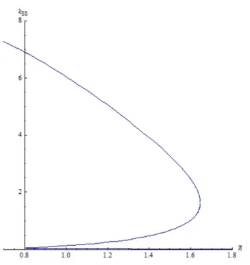
Consider the following set of parameters:
A = 3; = 3=4; = 0:85; = 2=3; = 4=5
In Figure 1, the bifurcation diagram is presented. It turns out that the critical values for are 1 = 0:806637and 2 = 1:64558. As long as < 0:806637, i.e. before
bifurcation occurs, there is only one steady state, xh, which is globally stable. As
slowly increases, the steady state capital stock decreases.
For = 0:806637 , an additional steady state appears in addition to xh and the
dynamics are now characterized by two steady states, xm < xh such that xh is locally
stable and xm is unstable in the sense that it is stable from the left but unstable from
the right.
When slightly increases from its critical value 0:806637, the unstable steady state splits into one locally stable and one unstable steady state through the saddle-node
bifurcation resulting in three steady states, xl(stable)< xm(unstable)< xh(stable), in
total. The coexistence of these three steady states is preserved until = 1:64558. As the value of gets closer to the critical value 1:64558, the highest stable steady state and the unstable steady state approach one another and at the critical value, they merge into a non-hyperbolic steady state. Slightly above the critical value, the non-hyperbolic steady state ceases to exist leaving only the stable steady state, xl
which is now globally stable. Further increases in only a¤ects the value of the stable steady state.
In sum, two types of the saddle-node bifurcation emerge. The di¤erence lies in the following: In the …rst one, the saddle-node bifurcation is realized for the pair of steady states xm and xh and in the second, it is for the pair of steady states xl
and xm. Moreover, in the …rst one, as increases, a pair of stable and unstable
steady states emerges simultaneously from a non-hyperbolic steady state and in the second, the qualitative change is in the form of coalescence of the steady states into a non-hyperbolic steady state.
This result signi…es the importance of the price of future oriented capital stock on the dynamic behavior of the system. The possibility of multiple steady states were established numerically for speci…c functional forms in Stern (2006). However, with the same functional forms, only by changing the value of , one can also obtain global convergence.
In this chapter, we consider the e¤ects of the relative cost of the future oriented capital on economic variables in the long term. In particular, we demonstrate the occurrence of a saddle-node bifurcation with respect to the price of future oriented capital stock. This is worth to examine optimal growth model with endogenous time preference while relaxing the assumption that the cost of the future-oriented
Figure 1: Bifurcation analysis for variations in
capital is constant. Assuming that it changes with wealth would lets us consider the factors in‡uencing the opportunity cost of time and e¤orts being assigned for the accumulation of future oriented capital stock. This is in our future agenda.
CHAPTER 3
STRATEGIC INTERACTION AND DYNAMICS UNDER
ENDOGENOUS TIME PREFERENCE1
To account for development patterns that di¤er considerably among economies in the long run (Quah, 1996; Barro, 1997; Barro and Sala-i-Martin, 1991), a va-riety of one-sector optimal growth models that incorporate some degree of market imperfections have been presented. These are based on technological external ef-fects and increasing returns (Dechert and Nishimura, 1983; Mitra and Ray, 1984) or the endogeneity of time preference (Becker and Mulligan, 1997; Stern, 2006; Erol et al., 2011). They have characterized the optimal paths and proven the emergence of threshold dynamics according to which the economies with low initial capital stocks or incomes converge to a steady state with low per capita income, while economies with high initial capital stocks converge to a steady state with high per capita income (see Azariadis and Stachurski, 2005, for a survey). However, to what extent these analyses are robust to the considerations of strategic interactions among agents in the economy, still remains as a concern.
1This essay is our joint work with Carmen Camacho and Ça¼gr¬Sa¼glam and published in Journal
This paper presents a strategic growth model with endogenous time preference. Each agent, receiving a share of income which is increasing in her own capital stock and decreasing in her rival’s, invests over an in…nite horizon to build her stocks. The heterogeneity among agents arises from di¤erences in their initial endowment, their share of aggregate income, and therefore in their subjective discount rates. We adopt the noncooperative open loop Nash equilibrium concept, in which players choose their strategies as simple time functions and they are able to commit themselves to time paths as equilibrium strategies. In this setup, agents choose their strategies simultaneously and each agent is faced with a single criterion optimization problem constrained by the strategies of the rival taken as given. We focus on the qualita-tive properties of the open-loop Nash equilibria and the dynamic implications of the strategic interaction.
In line with the empirical studies concluding that the rich are more patient than the poor (see Lawrence, 1991, and Samwick, 1998) and in parallel to the idea that the stock of wealth is a key to reach better health services and better insurance markets, we consider that the discount factor is increasing in the stock of wealth. However, this implies that the objective function of each agent’s single criterion optimization problem includes a multiplication of the discount function. This generally destroys the usual concavity argument which is used in the proof of the di¤erentiability of value function and the uniqueness of the optimal paths (see Benveniste and Scheinkman, 1979; Araujo, 1991).
Due to this potential lack of concavity and the di¤erentiability of the value func-tions associated with each agent’s problem, we employ the theory of monotone com-parative statics and the supermodular games based on order and monotonicity prop-erties on lattices (see Topkis, 1998). The analyses on the propprop-erties of supermodular games have been extensively concentrated in static games and to some extent in
dy-namic games with stationary Markov strategies (see Cooper, 1999; Amir, 2005; Vives, 2005, for a general review). This may stem from the fact that the use of open-loop strategies has been noted for being static in nature, not allowing for genuine strategic interaction between players during the play of the game. There are, however, many situations in which players lack any other information than their own actions and time so that the open-loop strategies can turn out to be unavoidable. The players may be unable to observe the state vector, let alone the actions of their rivals. In this respect, showing how the supermodular game structure can be utilized in the analysis of the dynamic games under open loop strategies is inevitable.
In this paper, we …rst provide the su¢ cient conditions of supermodularity for dynamic games with open-loop strategies based on two fundamental elements: the ability to order elements in the strategy space of the agents and the strategic com-plementarity which implies upward sloping best responses. In our dynamic game the open-loop strategies are vectors instead of simple scalars. Hence, the game requires an additional restriction to guarantee that all components of an agent’s best response vector move together. This explains the role of the restriction that the payo¤ function of each agent has to be supermodular in his own strategy given the strategy of his rival. The supermodular game structure of our model let us provide the existence and the monotonicity results on the greatest and the least equilibria. We sharpen these results by showing the di¤erentiability of the value function and the uniqueness of the best response correspondences almost everywhere. These allow us to derive conclusions on the nature of best responses, the set of equilibria and the long-run dynamics.
In particular, we analyze to what extent the strategic complementarity inherent in agents’strategies can alter the convergence results that could have emerged under a single agent optimal growth model and try to answer the following questions: Can
an agent with a larger initial stock credibly maintain this advantage to preempt the rival’s investment and reach a better long-run stock of capital? Put di¤erently, is the initial dominance reinforced by the actions of the agents? Can small initial di¤erences be magni…ed and then propagated through time? Can this kind of initial advantages vanish in the non-cooperative equilibrium of this class of games with strategic complementarity? Can the agent with a low initial capital stock pull the rich to her lower steady state that she would never face while acting by herself? Under what conditions do we have a unique equilibrium with strategic complementarity under open-loop strategies?
The key feature of our analysis is that the stationary state Nash equilibria tend to be symmetric under open-loop strategies. We show that the initially rich can pull the poor out of poverty trap even when sustaining a higher level of steady state capital stock for itself. A remarkable feature of our analysis is that it does not rely on particular parameterization of the exogenous functions involved in the model. Rather, it provides a more ‡exible framework with regards to the discounting of time, keeps the model analytically tractable and uses only general and plausible qualitative properties.
This chapter is organized as follows. The next section introduces the model. Tools needed while utilizing the supermodularity of the game; equilibrium dynamics and the steady state analysis have been discussed in Section 3.
3.1
The Model
We consider an intertemporal one sector model of a private ownership economy à la Arrow-Debreu with a single good xt, and two in…nitely lived agents, i = 1; 2: The
presumed to be supplied in …xed amounts, and the capital and consumption are in-terpreted in per-capita terms. The production function is given by f (xt) :We assume
that each agent receives a share of income i(xi t; x j t) = xi t xi t+x j t ; which is increasing in her own capital stock xi
t; and decreasing in her rival’s, x j
t. The amount of current
resources not consumed is saved individually as capital until the next period. For a given strategy of the rival, each agent chooses a path of consumption ci =fcitgt 0so as to maximize the discounted sum of instantaneous utilities, P1t=0 Qts=1 (xi
s) ui(cit)
where the functions u and denote the instantaneous utility from consumption and the level of discount on future utility, respectively.
In accordance with these, the problem of agent i can be formalized as follows:
max fci t;xit+1g 1 t=0 1 X t=0 t Y s=1 (xis) ! ui(cit); (P) subject to cit+ xit+1 i(xit; xtj)f (xit+ xjt) + (1 )xit;8t; cit 0; xit 0;8t; (xi0; xj0) 0; xj =fxjtg1t=1 0;given,
where j 6= i 2 f1; 2g; and 2 (0; 1) is the depreciation rate of the capital stock. Agents may only di¤er in their initial endowment, their share of output, and therefore in their subjective discount rates.
We make the following assumptions regarding the properties of the discount, utility and the production functions.
Assumption 3.1 : R+ ! R++ is continuous, di¤erentiable, strictly increasing
Assumption 3.2 u : R+ ! R+ is continuous, twice continuously di¤erentiable and
satis…es either u(0) = 0 or u(0) = 1: Moreover, u is strictly increasing, strictly concave and u0(0) = +1 (Inada condition).
Assumption 3.3 f : R+ ! R+ is continuous, twice continuously di¤erentiable and
satis…es f (0) = 0. Moreover, f it is strictly increasing and limx!+1f0(x) < .
We say that a path for capital xi = (xi1; xi2; :::) is feasible from (xi0; x j
0) 0; if for
all t and given xj 0; if for any t 0; xi satis…es that 0 xit+1 g(xit; x j
t) where
gi(xit; xjt) = i(xit; xjt)f (xit+ xjt) + (1 )xit:
Si(x
j) denotes the set of feasible accumulation paths from (xi0; x j
0): A consumption
sequence ci = (ci0; ci1; :::) is feasible from (xi0; x j
0) 0; when there exists a path for
capital, xi 2 Si(xj) with 0 cit gi(xit; x j
t) xit+1: As the utility and the discount
functions are strictly increasing, we introduce function U de…ned on the set of feasible sequences as U (xi j xj) = 1 X t=0 t Y s=1 (xis) ! u gi(xit; xjt) xit+1 :
The preliminary results are summarized in the following lemma which has a standard proof using the Tychonov theorem (see Le Van and Dana, 2003; Stokey and Lucas, 1989).
Lemma 3.1 Let x be the largest point x 0 such that f (x) + (1 )x = x. Then, for any xi in the set of feasible accumulation paths we have xit A(xi0+ x
j 0) for all t; where A xi0+ x j 0 = max xi0+ x j
0 ; x : Moreover, the set of feasible accumulation
paths is compact in the product topology de…ned on the space of sequences xi and U
In a recent paper, Erol et al. (2011) study the dynamic implications of the endoge-nous rate of time preference depending on the stock of capital in a single consumer one-sector optimal growth model. They prove that even under a convex technology there exists a critical value of initial stock, in the vicinity of which, small di¤erences lead to permanent di¤erences in the optimal path: economies with low initial capital stocks converge to a steady state with low per capita income. On the other hand, economies with high initial capital stocks converge to a steady state with high per capita income. Indeed, it is shown that the critical stock is not an unstable steady state so that if an economy starts at this stock, an indeterminacy will emerge.
In this paper, we propose a capital accumulation game where heterogeneous agents consume strategically. Heterogeneity arises from di¤erences in their initial endow-ment, their share of aggregate income, and therefore in their subjective discount rates. Our interest focuses on the qualitative properties of the open-loop Nash equilibria and the dynamic implications of the strategic interaction.
3.2
Non-Cooperative Di¤erence Game and Open-Loop
Nash Equilibrium
The noncooperative game in consideration is a triplet (N; S; fUi : i
2 Ng) where N = f1; 2g is the set of players, S = i2NSi is the set of joint admissible strategies under
open-loop information structure and Ui is the payo¤ function de…ned on S for each player i 2 N; i.e., Ui = U (x
i j xj) :
Any admissible strategy for agent i is an in…nite sequence compatible with the information structure of the game which is constant through time and restricted with the initial pair of capital stock in the economy. Accordingly, the set of admissible strategies for agent i; can be written as Si = 1
t=1Sti; where Sti = 0; gi(exit 1;ex j t 1) ;
with exi
t 1 = sup St 1i ; and ex j
t 1 = sup S j
t 1: Indeed, any strategy xi 2 Si is such that
xi t2 Sti;8t where S1i = 0; gi(xi0; x j 0) ; S2i = 0; gi gi(xi0; x j 0); gj(xi0; x j 0) ; :::; etc.
A few important remarks on the way the set of joint admissible strategies is constructed are in order. Denoting the set of joint feasible strategies by ; for any (xi; xj)2 ; we have (xi; xj) = [xj2XjS i(x j) [xi2XiS j(x i) \ ;
where Xj = fxj : Si(xj)6= ?g. It is important to recall from Topkis (1998) that
= [xj2XjS i(x
j) ([xi2XiS j(x
i))if and only if (xi; xj) = for each (xi; xj)
in : However, note that under the open-loop information structure of our game, the action spaces of the agents turn out to be dependent on each other converting the game into a “generalized game” in the sense of Debreu (1952). More precisely,
6= [xj2XjS i(x
j) ([xi2XiS j(x
i))as the set of feasible accumulation paths from
(xi 0; x
j
0) of agent i is constrained by the choices of agent j. This simply prohibits to
order elements in the joint feasible strategy space and calls for additional restrictions on the plan of the game in proving the existence of an equilibrium and analyzing the long-run dynamics via order theoretical reasoning. The admissibility condition2
imposed on the set of feasible strategies of the agents allows to write the set of joint admissible strategies as a simple cross product of the each agent’s set of admissible strategies that constitute a complete lattice.3
2Whenever there exists a positive externality, i.e., @gi(xi t;x
j t)
@xjt 0; 8t; the admissibility imposed
on the set of joint feasible strategies is far from a restriction. Even in case of negative externality, i.e., @gi(xit;x
j t)
@xjt < 0; 8t; the long-run implications of our analysis will not rely on such a restriction.
Indeed, an admissible strategy of agent i is an in…nite sequence of capital stock feasible from (xi0; xj0)
constituted under the consideration of the highest feasible strategy of the rival.
3In order to be able to work on a joint strategy space which constitutes a complete lattice, one
may also introduce an ad-hoc rule that exhausts the available stock of capital at the period where the joint strategies of the agents turn out to be infeasible (see Sundaram, 1989). However, in such a case, showing that the payo¤ function of each agent exhibits "increasing …rst di¤erences" on the joint strategies turns out to be unnecessarily complicated.
We adopt the noncooperative open loop Nash equilibrium concept, in which play-ers choose their strategies as simple time functions and they are able to commit themselves to time paths as equilibrium strategies. In this setup, agents choose their strategies simultaneously and each agent is faced with a single criterion optimization problem constrained by the strategies of the rival taken as given.
For each vector xj 2 Sj;the best response correspondence for agent i is the set of
all strategies that are optimal for agent i given xj :
Bri(xj) = arg max xi2Si
U (xi j xj) :
A feasible joint strategy (xi; xj) is an open loop Nash equilibrium if
U xi j xj U xi j xj for each xi 2 Si and each i 2 N: (22)
Given an equilibrium path, there is no feasible way for any agent to strictly improve his life-time discounted utility as the strategies of the other agent remains unchanged. The set of all equilibrium paths for this noncooperative game (N; S; fUi : i
2 Ng) is then identical to the set of pairs of sequences, (xi; xj) such that
xi 2 Bri xj and xj 2 Br j
(xi) : (23)
We will …rst prove that the best response correspondence of each agent is non-empty so that there exists an optimal solution to problem P. The dynamic properties of the best response correspondence then follows from the standard analysis in optimal growth models (see Stokey and Lucas, 1989; Le Van and Dana, 2003 and Erol et al., 2011) .