Design of 31-mode free-flooded ring transducers

(1)

DESIGN OF 31-MODE FREE-FLOODED

RING TRANSDUCERS

A THESIS

SUBMITTED TO THE DEPARTMENT OF ELECTRICAL AND ELECTRONICS ENGINEERING

AND THE INSTITUTE OF ENGINEERING AND SCIENCES OF BILKENT UNIVERSITY

IN PARTIAL FULLFILMENT OF THE REQUIREMENTS FOR THE DEGREE OF

MASTER OF SCIENCE

By

Sacit Yılmaz

December, 2008

(2)

ii

I certify that I have read this thesis and that in my opinion it is fully adequate, in scope and in quality, as a thesis for the degree of Master of Science.

Prof. Dr. Hayrettin Köymen (Supervisor)

Prof. Dr. Ayhan Altıntaş

Prof. Dr. Cevdet Aykanat

Approved for the Institute of Engineering and Sciences:

Prof. Dr. Mehmet Baray

(3)

iii

ABSTRACT

DESIGN OF 31-MODE FREE-FLOODED RING

TRANSDUCERS

Sacit Yılmaz

M.S. in Electrical and Electronics Engineering Supervisor: Prof. Dr. Hayrettin Köymen

December 2008

In this work, design and electromechanical analysis of radially polarized 31-Mode free-flooded ring transducers which have high power capability in deep submergence are explained. 31-Mode free-flooded ring transducers have Helmholtz resonance caused by the water inside, besides the radial resonance. By adjusting the dimensions of the ring, these resonance frequencies can be changed to the preferred values and desired band characteristics can be obtained.

Transducer is designed using circuit theory techniques on the electrical equivalent circuit of free-flooded ring. The ring transducer is modeled in ANSYS, a Finite Element Modeling tool. The results obtained by analyzing the electrical equivalent circuit and the ANSYS outputs are compared. Electrical equivalent circuit parameters are updated considering the result obtained in finite element analysis. Effects of mounting end tubes are investigated by finite element analysis. New components related to the end tubes are inserted to the electrical equivalent circuit.

(4)

iv

ÖZET

31-MODU AÇIK SİLİNDİR TÜP YAPILI TRANSDÜSER

TASARIMI

Sacit Yılmaz

Elektrik ve Elektronik Mühendisliği Bölümü Yüksek Lisans Tez Yöneticisi: Prof. Dr. Hayrettin Köymen

Aralık 2008

Bu çalışmada, derin sularda yüksek güç kapasitesi olan 31-modu açık (free-flooded) silindir tüp yapılı (ring) dönüştürücü (transducer) tasarımı ve elektromekanik analizi anlatılmaktadır. Açık silindir tüp dönüştürücülerde, tüpün radyal rezonansının yanısıra iç hacimde oluşan ve Helmholtz rezonansı olarak anılan bir rezonans daha vardır. Tüp boyutları doğru seçilerek bu iki rezonansın frekansları ayarlanabilir ve istenen band karakteristiği elde edilebilir.

Açık silindir tüp dönüştürücü tasarımı bant gereklerine göre elektriksel eşdeğer devre üzerinden yapıldı. Analiz aşamasında, tasarlanan açık tüp dönüştürücü sonlu eleman modelleme (SEM) yöntemini kullanan ANSYS programında modellendi. Eş değer devre çözümlemesinden elde edilen sonuçlar ile ANSYS’de elde edilen sonuçlar karşılaştırıldı. Sonlu eleman analizlerinde elde edilen sonuçlar dikkate alınarak elektriksel eşdeğer devre değiştirildi. Sonlu eleman analizleri ile eklenen montaj tüplerinin etkisi araştırıldı. Montaj tüplerinin etkisi dikkate alınarak elektriksel eşdeğer devre değiştirildi.

Anahtar Kelimeler: 31-mod açık silindir tüp yapılı dönüştürücü, ANSYS, Sonlu eleman modellemesi, SEM

(5)

v

Acknowledgements

I gratefully thank Prof. Dr. Hayrettin Köymen for his invaluable supervision, guidance and encouragement through the development of this thesis.

I would like to thank to my friends Zekeriyya and Aykut for valuable discussions. I would also like to thank to Niyazi Şenlik and Serhan Özsoy for their valuable help in FEM simulations, ANSYS.

I would like to express my endless thanks to my family for their loving support and being with me all the time.

(6)

vi

List of Figures

Figure 2.1 31-Mode Free-flooded ring transducer ... 7

Figure 2.2 Expansion of ring circumference ... 8

Figure 2.3 Radial Force ... 8

Figure 3.1 Electrical equivalent circuit of 31-mode free-flooded ring transducer ... 13

Figure 3.2 Free-flooded ring with half plane symmetry... 15

Figure 3.3 Input conductance-susceptance graph of the sample design (in MATLAB)... 17

Figure 3.4 ANSYS model of sample design ... 19

Figure 3.5 Conductance curve of sample design... 20

Figure 3.6 Susceptance curve of sample design... 20

Figure 3.7 Free-flooded ring transducer with mutual radiation impedance ... 21

Figure 3.8 New model to calculate port velocity ... 23

Figure 3.9 Electrical Equivalent Circuit with ports cannot move in y-direction and there exist water inside ... 25

Figure 3.10 Electrical Equivalent Circuit with ports cannot move in y-direction and there is no water inside ... 26

Figure 3.11 Mutual radiation impedance between port and outer cylindrical surface ... 27

Figure 3.12 Real parts of outer surface radiation impedances (Ansys result and sphere approxmation) ... 28

Figure 3.13 Imaginary parts of outer surface radiation impedances (Ansys result and sphere approximation) ... 29

Figure 3.14 Real parts of port radiation impedances (Ansys result and piston approximation) ... 30

Figure 3.15 Imaginary parts of port radiation impedances (Ansys result and piston approximation)... 31

Figure 3.16 Conductance-susceptance curve for correct values of radiation impedances ... 32

Figure 3.17 Outer surface to port acoustical transformer turns ratio ... 33

Figure 3.18 Acoustical turns ratio (first solution) ... 34

Figure 3.19 Acoustical turns ratio (second solution) ... 35

Figure 3.20 Turns ratio for correct input conductance-susceptance graph ... 36

Figure 3.21 Phase angle of transformer ratio for correct input conductance-susceptance graph... 37

Figure 3.22 Pressure at 20 cm distance ... 38

(9)

ix

Figure 4.1 Free-flooded ring transducer... 40

Figure 4.2 Free-flooded ring transducer with mounting end tubes ... 41

Figure 4.3 Electrical Equivalent Circuit of Transducer with end Tubes ... 42

Figure 4.4 Conductance-susceptance graph of sample design with end tubes... 45

Figure 4.5 Conductance vs. Frequency ... 46

Figure 4.6 Susceptance vs. Frequency ... 46

Figure 4.7 Displacement profile of transducer with end tubes... 48

Figure 4.8 Conductance vs. Frequency ... 49

Figure 4.9 Susceptance vs. Frequency ... 49

Figure 4.10 Pressure response of transducer with end tubes... 51

Figure 4.11 TVR (dB re 1µpa/V at 1m) ... 51

Figure II.1 Sample Conductance Curve ... 58

(10)

x

List of Tables

Table 1.1 Analogy between electrical and mechanical parameters... 3

Table 3.1 Electrical equivalent circuit parameters ... 13

Table 4.1 Dimensions of Sample Design ... 44

Table I.1 PZT-IV Material Properties ... 54

Table I.2 Properties of Stainless Steel... 54

Table I.3 Properties of Water ... 55

(11)

1

Chapter 1 Introduction

SONAR (Sound NAvigation and Ranging) technology is extremely important for naval systems to be protected against underwater threats such as a submarine, a torpedo or even an iceberg in terms of detection, localization and identification of the threat. For detection of a threat, SONAR uses underwater acoustic sound that is emitted by the target. Transducer is an element that is placed at the wet-end of SONAR. It converts the acoustical signal into an electrical signal that is transmitted to the dry-end side to be processed and vice versa. Many different types of transducers depending on frequency band requirements, shape limits, operating depth etc. are designed. In this thesis, we are interested in the design of 31-mode free-flooded ring transducers. This type of transducers is important to have a wide frequency band and can fully perform up to the full ocean depth.

1.1 Organization of Thesis

In Chapter 1, analogy between electrics and mechanics is given briefly. Piezoelectric materials are shortly explained and reason to use PZT-IV material for design of 31-mode free-flooded ring transducer is discussed. Some basic definitions in the field of underwater acoustics and transducer design are given. Difference of free-flooded ring transducer among other types of transducers is mentioned.

(12)

2

In Chapter 2, fundamentals of 31-mode free-flooded ring transducer are presented. Previous works on free-flooded ring transducers are summarized.

In Chapter 3, electrical equivalent circuit of 31-mode free-flooded ring transducer is introduced. A sample transducer is designed. Mismatch between electrical equivalent circuit and finite element analysis is discussed. Exact values of radiation impedances are calculated from finite element analysis. Transmitting voltage response of the transducer is represented.

In Chapter 4, some study on mounting of free-flooded transducer is performed. Stainless Steel mounting end tubes are attached to a free-flooded ring transducer. Change in vibration characteristics is observed. Change in band characteristics is discussed.

In Chapter 5, as a future work, formulation of electrical equivalent circuit parameters is proposed.

1.2 Analogy between Electrics and Mechanics

Transducer design is usually performed by electrical engineers, therefore, design of a transducer starts with some initial work on electrical equivalent circuit of a transducer. As a transducer takes acoustical sound as mechanical vibrations and converts this mechanical vibration into electrical signals, it is important to determine the analogy between electrical and mechanical parameters.

Some electrical parameters and their correspondences in mechanics are shown in Table 1.1 [1].

(13)

3

Table 1.1 Analogy between electrical and mechanical parameters Electrical Parameter Mechanical Parameter

Voltage V Force F

Current I Velocity υ

Capacitance C Compliance Cm

Inductance L Mass M

Charge C Displacement d

1.3 Piezoelectricity and Piezoelectric Materials

Recently piezoelectric materials are used to construct many types of transducers. Piezoelectric effect was first demonstrated by Pierre and Jacques Curie brothers [2] in 1880. They demonstrated the production of electricity when stress is applied to a piezoelectric material (direct piezoelectric effect); however, the converse piezoelectric effect (the production of stress and/or strain when an electric field is applied) was first discovered by Gabriel Lippmann [3] in 1881.

There exist both natural and man-made piezoelectric materials. Some natural crystals with piezoelectric effect are berlinite, cane sugar, quartz, Rochelle salt and topaz. Man-made piezoelectric materials include crystals like gallium orthophosphate and Langasite and ceramics such as barium titanate, lead titanate, lead zirconate titanate (PZT), potassium niobate, lithium niobate and lithium tantalite. Most commonly used piezoelectric material is PZT which has several types. Morgan [4], which is piezoelectric ceramic manufacturer, gives properties of many types of ceramics.

(14)

4

Main piezoelectricity ceramics that are introduced by Morgan Electro Ceramics are “Ceramic B”, “PZT-2”, “PZT-4”, “PZT-5A”, “PZT-5H” and “PZT-8”. Other ceramic manufacturers have corresponding materials also.

PZT-IV is the most suitable piezoelectric material for the design of high power and wideband 31-mode free-flooded ring transducers. PZT-IV has high power handling capability, low dielectric losses under high electric drive. Moreover, PZT-IV has high dielectric strength and it can withstand high mechanical stress.

1.4 Some Definitions

Quality Factor: Quality factor is the measure of a transducer that determines the width of 3 dB band of transducer depending on the center operating frequency. As quality factor increases, transducer has narrower operating band. This relation can be shown by the formula (1.1)

3 c dB f Q BW = (1.1)

In this works, we aim to design a low-Q, in other words, wideband transducer.

Transmitting Voltage Response (TVR): Transmitting voltage response is the ratio of pressure (µPa) generated at 1m distance from transducer to the input voltage (V). This ratio is usually presented in logarithmic form. Transmitting voltage response can be formulated as:

1 P ( ) ( ) 20 log( m ) input Pa TVR dB V

µ

= (1.2)

(15)

5

Specific Acoustic Impedance (ρc): Specific acoustic impedance is the multiplication of density and sound speed. For water this identity is shown to be ρ0c0 and this value equals to 1.5 Mrayl.

1.5 Free-Flooded Ring Transducers

Free-flooded ring transducers are ideally suited for, high power, broadband (low-Q) sound generation. Performance of this type of transducers does not change much depending on the hydrostatic pressure. Therefore, free-flooded ring transducers can fully perform up to the full ocean depth. It should also be noted that free-flooded ring transducers are easy to be produced. As a result, they are low-cost. However, it is a problem for free-flooded ring transducers to be mounted as they have no nodal point during vibration. In Chapter 4, solution to the problem of mounting is discussed.

(16)

6

Chapter 2 Fundamentals of Free-Flooded Ring

Transducers

Radially polarized ring transducers vibrate at the frequency same as the AC voltage applied between electrical input terminals. In a particular frequency this radial vibration reaches a resonance. This resonance frequency is called as “ring resonance”. For free-flooded ring transducers, there exists another type of resonance called “Helmholtz resonance” besides the radial resonance. While the ring extends, the surrounding water is compressed and the water inside expands, therefore, surrounding water gets inside the transducer. On the other hand, as the ring shrinks water inside is compressed and surrounding water expands, therefore, water inside the transducer goes to the outside of the transducer. The combination of motions of inner and outer water causes cancellation in the radial direction due to 180º phase difference. However, this cancellation cannot create null in the radial direction because of different inner and outer areas and small thickness and height mode radiation from transducer. At a particular frequency this radial radiation reaches to a maximum. This frequency is called “Helmholtz frequency” or “cavity resonance frequency”.

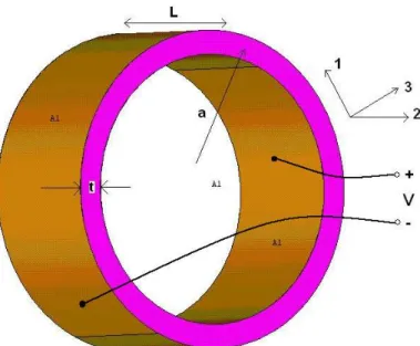
The shape of a 31-mode free-flooded ring transducer is illustrated in Figure 2.1. The electrical polarization of the ring is in the 3 direction, radial direction. Electric fields in the 1 and 2 direction (E₁,E ) are zero. The direction in which ₂ stress is continuous along is 1. Considering the directions of both electric field and stress, this transducer is called as “31-mode”.

(17)

7

Figure 2.131-Mode Free-flooded ring transducer

When the thickness of the ring is small compared to the mean radius (t << a) and the length is small compared to the mean diameter (L << 2a), moreover, when the ends are assumed to be free to move (T2 = 0), the piezoelectric equation pair for

the ring transducer can be written as: 1 11 1 31 3 E S =s T +d E (2.1) 3 31 1 33 3 T D =d T +ε E (2.2)

where S is strain, D is electric field density, T is stress and E is electric field. On the other hand, s is compliance coefficient, d is piezoelectric coefficient and ε is the permittivity coefficient. Note that, values of these coefficients for PZT-4 material are given in Appendix-I.

(18)

8

Figure 2.2 Expansion of ring circumference

In Figure 2.2, how the ring transducer expands is illustrated. Starting from Equation 2.1, circumferential strain can be developed as:

11 31

/a s F tL/ d V t/

ξ

= + (2.3)

F can be related to Fr as shown in Figure 2.3.

Figure 2.3 Radial Force

For small values of δθ, F_r =2 sin(F

δθ

/ 2)≈F

δθ

, and, this applies to every point around the ring, therefore, total radial force becomes F_r =2

π

F.

(19)

9

Moreover, for small displacements, the ring moves as a mass, M =ρ π2 atL, and the radial equation of motion is

..

0 r 0 2

Mξ =F −F =F − πF (2.4)

where F0 is any additional force, expect the internal moving force, such as the

force due to radiation.

Substitution of F from Eq. (2.3) into Eq. (2.4) leads to the equation:

..

0 E

Mξ+K ξ =NV +F (2.5)

where KE =2πtL s a/ ₁₁E is the short circuit radial stiffness and N =2πLd₃₁/s₁₁E is the electromechanical turns ratio. Considering the sinusoidal conditions, Eq. (2.5) will be

. .

0

( E/ )

jwMξ+ K jw ξ =NV +F (2.6)

As F0 includes both the radiation impedance, Zr, and the mechanical damping

resistance, Rm, the velocity in the radial direction, .

u= , on the ring will be ξ /( E/ _m _r)

u=NV jwM +K jw+R +Z (2.7)

where NV, input voltage multiplied by the electromechanical turns ratio, is the piezoelectric driving force in the radial direction.

As Rm is the mechanical loss resistance, can be neglected, and Zr is negligible

for air-loading conditions, the mechanical resonance occurs at the frequencyw2 =KE /M =1/s₁₁Eρa2. Considering the formula of bar wave speed,

1 2 11

(1/ E )

(20)

10 c w a = ⇒ 2 f c a π = ⇒ 2 a c f π = ⇒ 2 a c f π = ⇒ fD c π = (2.8) Then, it can be concluded thatthe mechanical ring resonance occurs when the wave length equals to the circumference of the ring. This equation can be specialized for PZT-4 (Navy Type I).

41

fD = kHz inches− (2.9)

2.1 Related Works on Free-Flooded Ring

Transducers

Free-flooded ring transducers were called as “squirters” during early development phase. The earliest analysis of free-flooded rings is done by Robey [5]. In his paper, Robey studied on the radiation loading of a free-flooded ring radiating from its open ends. He obtained the impedance presented to inside surface of the transducer. However, he did not consider the interaction between the inner and outer surfaces. In another work, Robey [6] studied on the radiation impedance of an array of free-flooded ring transducers.

McMahon [7] developed a theory that predicts the cavity resonant frequency of an open cylindrical shell immersed in water. With this theory, it is possible to predict the cavity resonant frequency for different ratios of ceramic height, thickness and radius.

Some other initial studies were conducted on the acoustic radiation and radiation pattern of the finite cylinder [8], [9].

In 1965, Junger [10] derived the mutual and self radiation impedances of an array of free-flooding ring transducers. He expressed the radiation impedance as the sum of two components: the impedance introduced by Robey and the impedance

(21)

11

that comes out of the radial velocity distribution over the two cylindrical surfaces. This radiation impedance given for a single transducer consists of complex integrals and it is not easy to solve. In another work, Junger [11] studied on the band responses of free-flooded ring transducers with respect to aspect ratio (height/radius) and ratio of sound velocities in water and in transducer.

Following studies on the radiation characteristics of free-flooded rings gave better theoretical results [12], [13], [14], [15].

In 1972, Rogers [16] introduced The Naval Research Laboratory SHIP which calculates acoustic surface pressures, radiation impedances, and far-field radiation patterns of finite cylinders and free-flooded rings. Besides the geometry of the ring or cylinder, the program needs the normal velocity distribution on the surface of the source.

In the next work, Rogers and Zalesak [17] generated tables of coefficients for calculating the radiation impedance and far-field pressure of a free-flooded ring. In their system, they expected the inside, bottom and top, and outside normal velocities to be uniform. Their tables included coefficients of 45 frequencies for 36 ring geometries.

In 1974, Finite Element Method (FEM) was used to model free-flooded ring transducers [18]. In this application, FEM analysis is used to compute normal velocity distribution on the boundaries of the transducer and the velocity distribution is used as input to CHIEF (Combined Helmholtz Integral Equation Formulation) which calculates the acoustic radiation impedance and pressure distribution.

In 1976, Butler [19] introduced a model for a ring transducer with inactive segments. Butler constructed tangentially polarized parallel wired segmented rings with inactive segments. He developed the equation of motion and the

(22)

12

electrical equivalent circuit for a segmented ring transducer which incorporates inactive segments.

In 1986, Rogers [20] created a further mathematical model for obtaining the transmitting response of a free-flooded, thickness-polarized piezoelectric cylinder transducer. In this model, Rogers used the outputs of SHIP as the radiation loads. Kuntsal [21] examined the model of McMahon by constructing arrays of free-flooded ring transducers. He compared the cavity resonance frequencies obtained from McMahon’s model and measurement data. Furthermore, Kuntsal investigated the effects of the end tubes on the free-flooded ring transducers.

(23)

13

Chapter 3 Electrical Equivalent Circuit Model

of

31-Mode

Free-Flooded

Ring

Transducer

Going through the piezoelectric equation pair which is given in the previous chapter, electrical equivalent circuit of 31-mode free-flooded ring transducer was obtained by Sherman and Butler [22] as shown in Figure 3.1.

Figure 3.1 Electrical equivalent circuit of 31-mode free-flooded ring transducer

Consistent with the electrical equivalent circuit given in Figure 3.1, formulation and definition of components are given in Table 3.1.

Table 3.1Electrical equivalent circuit parameters Parameter Formulation Definition

0

C 2π εaL ₃₃T /t Electrical input capacitance 33 T ε ₃₃T _{33 0}T K ε = ε Relative permittivity 0

(24)

14

N 2 31/ 11

E

Ld s

π Electromechanical turns ratio

E C _1/ 11 2 E E s a K tL π = Mechanical compliance

M ρ π2 atL Mass of transducer m

R Neglected Mechanical loss resistance 1

C 1

2 L

β π

Radial compliance of inner volume

n −a2/L

Acoustical transformer ratio from outer surface to port

2

R Neglected _{Mechanical loss at the ports}

r

Z

Radiation impedance of an equivalent sphere with the same

radiating area

Radiation impedance of outer cylindrical surface

p

Z Impedance of o piston in a finite

rigid baffle Port radiation impedance

3.1 Radiation Impedances

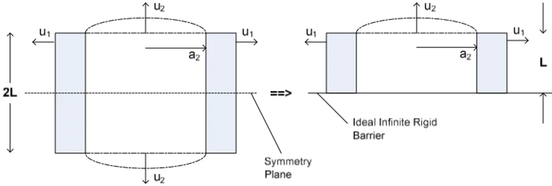
Model of a free-flooded ring transducer can be simplified making use of half plane symmetry which is illustrated in Figure 3.2. In the right hand side of the figure half plane model with an-only fluid port is shown.

(25)

15

Figure 3.2 Free-flooded ring with half plane symmetry

Considering the simplification, one port and one outer surface radiation impedances are placed in the electrical equivalent circuit model. Radiation impedance of the cylindrical outer surface (Zr) is modeled using the radiation

impedance of a sphere with the same radiating area. If it is noted that the radius of sphere with a same radiating area with half cylinder outer surface is

1/ 2 s

a =((a t+ / 2) / 2)L , radiation impedance of the outer half surface can be formulated as:

2 2

0 0[( s) s] /[1 ( s) ]

A cρ ka + jka + ka (3.1) where A is the area of the outer cylindrical half-plane surface.

In the electrical equivalent circuit model, piston in a rigid baffle approximation is used to calculate port radiation impedance (Zp) because of half-plane

symmetry and small length (L) compared to wavelength. Port radiation impedance is formulated by Blackstock [23] as:

1 1 0 0 (2 ) 2 (2 ) (1 2 ) 2 2 J ka K ka A c j ka ka ρ − + (3.2)

(26)

16

In this formula A is the area of the port. Imaginary part of the formula (3.2),

1

2 (2 ) 2 K ka

ka , can be calculated by the approximation (3.3)

3 5 1 2 2 2 4 2 (2 ) (2 ) ( ...) 3 3 5 3 5 7 ka ka ka X π = − + − (3.3)

3.2 Sample Design Using Electrical Equivalent

Circuit

Sample design has the dimensions such that a = 46 – t/2 mm, L = 42 mm and t = 10 mm. Piezoelectric material is chosen to be PZT-IV.

MATLAB is used for analyzing the electrical equivalent circuit. Calculating the electrical equivalent circuit parameters according to Table 3.1, input conductance-susceptance graph is obtained as shown in Figure 3.3.

(27)

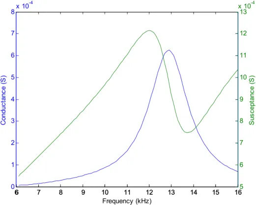
17 6 7 8 9 10 11 12 13 14 15 16 0 1 2 3 4 5 6 7 8x 10 -4 C o n d u c ta n c e ( S ) Frequency (kHz) 6 7 8 9 10 11 12 13 14 15 165 6 7 8 9 10 11 12 13 x 10-4 S u s c e p ta n c e ( S )

Figure 3.3Input conductance-susceptance graph of the sample design (in MATLAB)

In Figure 3.3, it is notable that there exists an only the ring resonance frequency which is about 13 kHz. If we use the formula (2.9) with D=2a=82 mm, resonance frequency turns out to be 12.7 kHz which is in close agreement with the electrical equivalent circuit analysis result. Then, some study on Helmholtz resonance frequency must be performed.

3.3 Application of McMahon’s Theory

The numerical formula to calculate Helmholtz frequency is first introduced by McMahon. According to McMahon’s theory, the cavity (Helmholtz) resonance frequency of a free-flooded ring transducer can be approximated by the formula:

(28)

18

2

( h / 2a + 0.633) - 0.106 π/ 2

Ω Ω = (3.4)

In this formula, h is the length, and a is the inside radius of transducer.

c 0

= w a / c

Ω is dimensionless frequency parameter. Because the velocity of sound within the tube is effectively less than the velocity of sound in open water, the correction formula:

1 2

0 11

c =c(1 2+ Ba Y t/ )− (3.5)

is inserted. In this formula, c is the speed of sound in open water and B is the bulk modulus of water. Y11 is the Young’s Modulus of Lead Zirconate Titanate.

The experimental value of 61 GPa is used for this parameter.

For the sample design, the cavity resonance frequency is calculated to be 8.7 kHz, which is in close agreement with the FEM analysis result.

The reason of this much difference between electrical equivalent circuit model and the ANSYS [24] analysis can be caused by the mutual radiation impedance between port and the outer surface of cylinder.

3.4 Finite Element Analysis of Sample Design

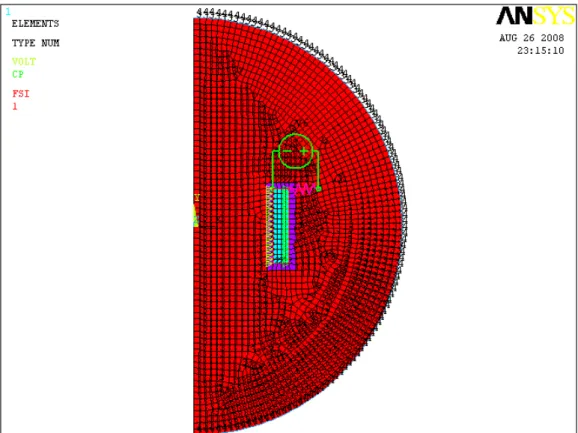
ANSYS is used for finite element analysis. Transducer is modeled using the axis-symmetric option [25]; therefore, 2D model of the transducer and inside and surrounding water are constructed. For water loading on transducer, fluid-surface interface (FSI) is created between the water and transducer fluid-surfaces touching to water. In order to eliminate the reflection effects of outer fluid boundary, absorbing boundary is constructed at the outer cylindrical fluid surface. PLANE13 [26] material for ceramic, PLANE29 material for water and PLANE129 material for absorbing boundary are used. Due to the definition of

(29)

19

the PLANE129 material there is no reflection back from the outer circle. Electrical circuit elements, voltage source and resistor, are selected to be CIRCU94 elements.

Figure 3.4ANSYS model of sample design

Simulating the sample transducer, conductance and susceptance curves are obtained as given in Figure 3.5 and Figure 3.6.

According to the conductance graph in Figure 3.5, 3 dB band is between 7.5 kHz and 15.2 kHz. Assuming 11.35 kHz to be the center frequency, Q-factor turns out to be 1.5 whish is a very low value.

(30)

20

Figure 3.5 Conductance curve of sample design

(31)

21

3.5 Electrical Equivalent Circuit with Mutual

Radiation Impedance

Electrical equivalent circuit of a free-flooded ring transducer with mutual radiation impedance (Zrp) is given as shown in Figure 3.7 by Sherman and

Butler [22].

Figure 3.7 Free-flooded ring transducer with mutual radiation impedance

In this circuit Zrp is the mutual radiation impedance between port and outer

cylindrical surface. On the other hand, Zr and Zp are the pure radiation

impedances of outer surface and port respectively. Because, Zrp is estimated to

be comparable with both Zr and Zp, it should be included in the electrical

equivalent circuit to obtain a complete model of the transducer.

It should be noted that there is no analytical formula to calculate the mutual radiation impedance of free-flooded ring transducer in the electrical equivalent circuit model. Then, mutual radiation impedance will be tried to be calculated from ANSYS simulation results.

(32)

22

3.6 How to Calculate Radiation Impedances Using

ANSYS results

Force matrix including both outer surface and port forces can be formulated as in formula (3.6): r rp r r p rp p p Z Z F F Z Z

υ

      =              (3.6)

According to this matrix formulation, port and outer surface forces can be written as:

r r r rp p

F =Z

υ

+Z

υ

(3.7)

p p p rp r

F =Z

υ

+Z

υ

(3.8)

Using these formulas, outer surface and port radiation impedances can be derived as: r rp p r r F Z Z

υ

− = (3.9) p rp r p p F Z Z

υ

− = (3.10)

It possible to obtain F_r, F and _p

υ

_rin the original ANSYS model. What to be done is to develop a new model for obtaining

υ

_p and calculating Z . _rp

3.7 New ANSYS Model to Obtain Port Velocity

To compare ANSYS model and electrical equivalent circuit model results, mutual and self radiation impedances of both port and cylindrical outer surface, average

(33)

23

velocities of both port and outer surface are needed to be calculated. On the other hand, ANSYS do not calculate displacement values for water elements. Therefore, port velocity distribution can not be obtained from the original model.

For port displacement values to be read, a new model must be constructed to simulate the radiating water at the port. This water was modeled using PLANE42 elements with material properties similar to water. The sketch of the model is illustrated in Figure 3.8. To calculate average velocity, average displacement on the port is calculated and average velocity is obtained by the formula:

υ

_average = jwd_average where w is the angular frequency and d_average is the average displacement on the port.

(34)

24

3.8 Mutual Radiation Impedance

Mutual coupling between outer surface and port is an important phenomenon for free-flooded ring transducers. To measure this coupling effect between port and outer surface is not possible. However, in the ANSYS model, it is possible to calculate the mutual impedance.

Working on formulas (3.9) and (3.10), mutual radiation impedance between port and outer surface can be formulated as in formulas (3.11) and (3.12):

0 p p rp r F Z _υ

υ

= = (3.11) 0 r r rp p F Z _υ

υ

= = (3.12)

If the formula (3.11) is preferred, ports must be forced not to move in y-direction. Transducer can be driven from the electrical ports. Then, the ratio of force on the port to the average velocity of outer cylindrical surface will be the mutual radiation impedance between port and the outer cylindrical surface. It is an important point to come to a decision whether there should be water inside the ring or not. At this point, it would be fine to mention what changes depending on the existence of water inside.

3.8.1 Mutual Radiation Impedance Calculation When

There Exist Water Inside

When there exists water inside the ring, water adds extra stiffness and it affects the force on the port. This effect can be visualized by the electrical equivalent

(35)

25

circuit which characterizes the situation that there exists water inside the transducer and ports are not permitted to move in y-direction in Figure 3.9.

Figure 3.9 Electrical Equivalent Circuit with ports cannot move in y-direction and there exist water inside

In this model, Zp radiation impedance does not exist because of non-existence of

propagation from the port. Because C1 simulates the compression and expansion

of water inside, Fp will not be a force purely caused by the vibration of the outer

surface. Therefore, to measure the mutual radiation impedance correctly, there should not be C1 capacitor. This capacitor must be open-circuited.

3.8.2 Mutual Radiation Impedance Calculation When

There Exist no Water inside Transducer

When there exists no water inside the ring, mutual effect between the port and the outer surface can be calculated without any interference. The electrical equivalent circuit when there is no water inside the transducer is shown in Figure 3.10. Moreover, port force and outer surface velocity are illustrated.

(36)

26

Figure 3.10Electrical Equivalent Circuit with ports cannot move in y-direction and there is no water inside

Interpreting this electrical equivalent circuit, it is obvious that mutual radiation impedance can be calculated by the formula (3.11) where port velocity is zero as it should be and Fp is the force which is purely caused by the radiation of water

from cylindrical outer surface.

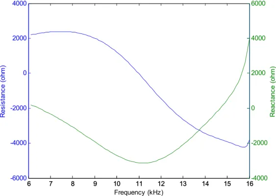
To calculate the mutual radiation impedance between outer cylindrical surface and port, transducer was modeled in ANSYS without water inside. Transducer was driven by the electrical voltage input and ports were not allowed to move in vertical direction. Dividing force on port to the average velocity of outer surface, mutual radiation impedance is obtained to be as shown in Figure 3.11.

(37)

27 6 7 8 9 10 11 12 13 14 15 16 -6000 -4000 -2000 0 2000 4000 R e s is ta n c e ( o h m ) Frequency (kHz) 6 7 8 9 10 11 12 13 14 15 16-4000 -2000 0 2000 4000 6000 R e a c ta n c e ( o h m )

Figure 3.11 Mutual radiation impedance between port and outer cylindrical surface

3.9 Comparison

of

Approximated

Radiation

Impedances and Finite Element Analysis

Results

Outer surface radiation impedance, Zr, is calculated by the formula (3.1) in the

electrical equivalent circuit model due to sphere approximation. On the other hand, in the finite element analysis Zr is calculated using the formula (3.9) in the

model of Figure 3.8. In Figure 3.12 and Figure 3.13 real and imaginary parts of sphere approximation and ANSYS results of outer surface radiation impedances are illustrated together respectively.

(38)

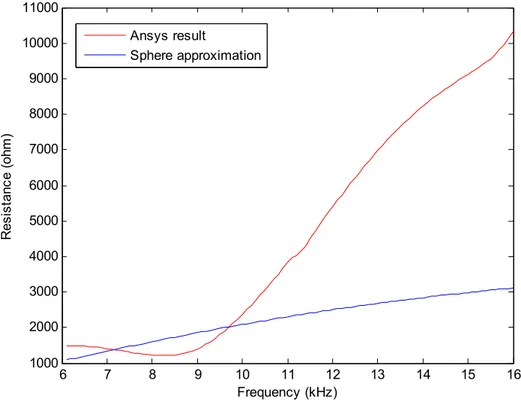
28 6 7 8 9 10 11 12 13 14 15 16 1000 2000 3000 4000 5000 6000 7000 8000 9000 10000 11000 Frequency (kHz) R e s is ta n c e ( o h m ) Ansys result Sphere approximation

Figure 3.12 Real parts of outer surface radiation impedances (ANSYS result and sphere approximation)

To interpret the graphs in Figure 3.12, real part of ANSYS result and Sphere approximation seem to be very similar about Helmholtz resonance frequency. However, about the ring resonance they are very different. ANSYS result seems to be three times sphere approximation.

(39)

29 6 7 8 9 10 11 12 13 14 15 16 1000 2000 3000 4000 5000 6000 7000 8000 9000 Frequency (kHz) R e a c ta n c e ( o h m ) Ansys result Sphere approximation

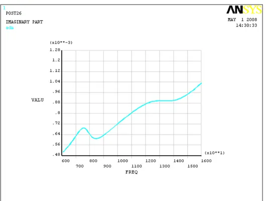
Figure 3.13 Imaginary parts of outer surface radiation impedances (ANSYS result and sphere approximation)

In Figure 3.13, it is seen that ANSYS result is about 3-4 times the sphere approximation. It should be noted that the imaginary part of outer surface radiation impedance is important to determine the ring resonance. Ring resonance frequency is determined not only by capacitance CE and inductance M, but also imaginary part of outer surface radiation impedance. In other words, CE resonates with M +imag Z( _r). Therefore, it is important not to predict imaginary part of outer surface radiation impedance wrongly.

Port radiation impedance, Zp, is calculated by formulas (3.2) and (3.3) in the

electrical equivalent circuit model due to piston in a rigid baffle approximation. On the other hand, in the finite element analysis Zp is calculated using the

(40)

30

and imaginary parts of piston approximation and ANSYS results are illustrated together. 6 7 8 9 10 11 12 13 14 15 16 2000 3000 4000 5000 6000 7000 8000 9000 10000 Frequency (kHz) R e s is ta n c e ( o h m ) Ansys result Piston approximation

Figure 3.14 Real parts of port radiation impedances (Ansys result and piston approximation)

According to the graphs in Figure 3.14, it can be seen that ANSYS result and piston approximation give very close results to each other about Helmholtz resonance. ANSYS result deviates from the piston approximation and becomes two times the piston approximation about the ring resonance. However, it should be noted that value of Zp is not that much important about the ring resonance

due to dominance of Zr. Then it can be concluded that piston approximation

(41)

31 6 7 8 9 10 11 12 13 14 15 16 -4000 -2000 0 2000 4000 6000 8000 Frequency (kHz) R e a c ta n c e ( o h m ) Ansys result Piston approximation

Figure 3.15 Imaginary parts of port radiation impedances (Ansys result and piston approximation)

Comparing the imaginary parts of port radiation impedances, it is seen that ANSYS result is about 50% more than the piston approximation result. However, it should be noted that imaginary part of port impedance is a determinant factor for Helmholtz resonance frequency. At the Helmholtz resonance frequency, C1

capacitor resonates with imaginary part of port radiation impedance transformed into outer surface. This relation can be formulated as:

1 2 1 ( ) 2 h p f imag Z C n

π

= (3.13)

Therefore, it is very important to predict imaginary part of port radiation impedance correctly. It can be concluded that piston in a rigid baffle approximation predicts the imaginary part of the port radiation impedance well.

(42)

32

3.10 Acoustical Transformer Turns Ratio

After radiation impedances are correctly obtained according to the ANSYS simulations, electrical equivalent circuit is analyzed in terms of input conductance and susceptance. This conductance-susceptance graphs are given in Figure 3.16. 6 7 8 9 10 11 12 13 14 15 16 0 0.5 1x 10 -3 C o n d u c ta n c e ( S ) Frequency (kHz) 6 7 8 9 10 11 12 13 14 15 160.5 1 1.5 x 10-3 S u s c e p ta n c e ( S )

Figure 3.16 Conductance-susceptance curve for correct values of radiation impedances

Conductance graph in Figure 3.16 shows that correct values of radiation impedances are not enough to obtain the same conductance-susceptance curve with ANSYS simulation. Especially, the Helmholtz resonance has to be investigated more. As C1 is the radial compliance of water inside, it should be

(43)

33 1 4 4 1 xArea rL L compliance length r

β

β π

= = = (3.14)

With the acceptance that C1 has the correct value, the only parameter to be

doubted on is the acoustical transformer ratio, n. This transformer ratio can be calculated from the equivalent electrical circuit part that is shown in Figure 3.17.

Figure 3.17 Outer surface to port acoustical transformer turns ratio

According to current division given in Figure 3.17, voltage on C1 capacitor can

be written as 1 2 1 p F u nu jwC n − − ₌ (3.15)

This equation can be converted into a second degree equation with one unknown such that:

2

2 1 1 p 0

u n −u n− jwC F = (3.16)

To solve turns ratio from this formula, results obtained from ANSYS for u , ₁ u ₂ and F , moreover, C_p 1 capacitor such that its value is calculated by the formula

(3.14) are used. Two different solutions for turns ratio are obtained. These solutions are shown in Figure 3.18 and Figure 3.19.

(44)

34 6 7 8 9 10 11 12 13 14 15 16 -0.6 -0.4 -0.2 0 0.2 0.4 0.6 0.8 1 1.2 Frequency (kHz) Real Imaginary

Figure 3.18 Acoustical turns ratio (first solution)

According to the graph in Figure 3.18, real part of turns ratio turns out to be zero somewhere in the 3 dB band of transducer. This means that somewhere in the 3 dB frequency band, real radiation of the port is not transformed into a radial radiation. This situation is not a result that is expected.

(45)

35 6 7 8 9 10 11 12 13 14 15 16 -3.5 -3 -2.5 -2 -1.5 -1 -0.5 0 0.5 1 Frequency (kHz) Real Imaginary

Figure 3.19Acoustical turns ratio (second solution)

In the graph in Figure 3.19, it is also seen that real part of turns ratio turns out to be zero also for the second solution.

It is obvious that for turns ratio cannot be zero somewhere in the 3 dB frequency band, C1 capacitor must have a complex value which is not possible. Therefore,

it will be a better way to compute the turns ratio from expected input admittance curves. In this calculation, it is assumed that some parameters given in the electrical equivalent circuit model are correct. These parameters are input capacitance (C0), electromechanical turns ratio (N), radial compliance of

transducer (CE), total mass of transducer (M) and radial compliance of inner water (C1). Moreover, for radiation impedances, Zr, Zp and Zrp, computed values

(46)

conductance-36

susceptance graph same as given in the Figure 3.5, outer surface to port acoustical transformer turns ratio turns out to be given as in Figure 3.20.

6 7 8 9 10 11 12 13 14 15 16 -1.4 -1.2 -1 -0.8 -0.6 -0.4 -0.2 0 0.2 0.4 0.6 Frequency (kHz) Real Imaginary

Figure 3.20 Turns ratio for correct input conductance-susceptance graph

It is seen in Figure 3.20 that acoustical turns ratio of transformer from outer surface to port can not be modeled by a transformer with a constant real value in the frequency band. This transformer seems to have a complex valued transformer ratio. The phase angle of this transformer ratio is shown in Figure 3.21.

(47)

37 6 7 8 9 10 11 12 13 14 15 16 156 158 160 162 164 166 168 170 172 174 Frequency (kHz) P h a s e a n g le ( d e g re e s )

Figure 3.21 Phase angle of transformer ratio for correct input conductance-susceptance graph

As it is seen in Figure 3.21, not only the absolute value of turns ratio but also the phase of turns ratio changes. This means that port and outer surface cannot be modeled as moving with 180º phase difference as presumed.

3.11 TVR of the Transducer

For TVR calculation, it is very important find the far-field pressure response of the transducer at the center of the main beam. After finding the pressure value, this pressure value is transformed into 1m distance equivalent. To calculate the transmitting voltage response, formula (1.2) is used.

(48)

38

To compute the far-field distance for designed transducer, the formula (3.17) which is given by Balanis [27] is used.

2 2 far field D d

λ

− = (3.17)

where D is the outer diameter for our transducer and λ is the wave length at the operating frequency. For wavelength, 15.5 kHz is taken which is the maximum frequency in the 3-dB band and diameter is 0.092 m. Then, far-field distance turns out to be 17.49 cm. Pressure profile at 20 cm distance from transducer is illustrated in Figure 3.22.

(49)

39

Pressure at 20 cm distance from transducer can be scaled into 1 m distance pressure by dividing by 5. The ratio of that pressure to the input voltage gives the transmitting voltage response of the transducer as illustrated in Figure 3.23.

(50)

40

Chapter 4 Mounting of Free-Flooded Ring

Transducers

Mounting is an important problem for free-flooded ring transducers because there is no non-vibrating point on the transducer. In this part, two alternative ways to mount the flooded ring transducers are mentioned. First, free-flooded ring can be immersed into the water without fixing it. Corresponding shape of the transducer is illustrated in Figure 4.1.

Figure 4.1Free-flooded ring transducer

The transducer that is shown in Figure 4.1 can be immersed into water with some cord wrapped around it. Black bars around the transducer are polymer components that cord can be wrapped.

The second alternative for mounting a free-flooded ring transducer is to extend the transducer with mounting end tubes. End tubes are developed with materials

(51)

41

that can be processed to have some screw holes. A free-flooded ring transducer with mounting end tubes is illustrated in Figure 4.2.

Figure 4.2 Free-flooded ring transducer with mounting end tubes

These end tubes are very important for transducer to be mounted; however, they should be carefully attached as they change the characteristics of the transducer.

4.1 Effects of End Tubes

End tubes are usually selected from stiff materials such as steel, brass or sometimes aluminum. These stiff and heavy materials are impossible not to change the characteristics of transducer. Considering properties of end tubes, effects of attaching end tubes to free-flooded ring transducers can be listed as:

• Increasing the total radial stiffness due to parallel spring effect of end tubes

• Increasing the total mass of transducer due to the intolerable mass of end tubes

• Increasing the mass of total radiating water inside the transducer due to the increase in the inside volume

(52)

42

• Decreasing the radial compliance of the water inside due to the increase in the cross-sectional area that water inside sees during radial motion

Considering these effects some other effects can be derived such as: • Helmholtz resonance frequency decreases

• Radial resonance frequency increases

4.2 Electrical Equivalent Circuit of Free-Flooded

Ring Transducer with End Tubes

Considering the effects listed in the previous section, the electrical equivalent circuit of free-flooded ring transducer has to be updated as shown in Figure 4.3.

R

2

Figure 4.3 Electrical Equivalent Circuit of Transducer with end Tubes

The only effect seen in the circuit schematics is added capacitor and inductor due to stiffness and mass of end tubes. However, other elements of equivalent circuit also changes due to total geometry change of the transducer. To mention about all the elements changing by the addition of the end tubes:

• K_tube : Total stiffness of two end tubes in the radial direction This value can be calculated by the formula K_tube = 2* *t*2*h*E_tube / a

π

where E_tube is the Young’s modulus of the tube material and h is the length of a single end tube.

(53)

43 • M_tube : Total mass of two end tubes

This value can be calculated by the formula M_tube = 2* *ro_tube*a*t*2*h

π

where ro_tube is the density of the tube material.

• Zr : Radiation impedance of the outer surface

As the outer surface of the transducer increases by addition of end tubes, it is expected the outer surface radiation impedance to change proportional to the length of transducer.

• C1 : Radial compliance of the inner volume

Because this value is inversely proportional to the length of transducer, as the length of the transducer increases by addition of end tubes, radial compliance of inner volume decreases.

• n : Port to outer surface turns ratio

Because this value is inversely proportional to the length of transducer, as the length of the transducer increases by addition of end tubes, port to outer surface turns ratio decreases.

Note that C0 which is an electrical parameter does not change. Moreover, N does

not change as it is related to type and shape of piezoelectric material.

While constructing the electrical equivalent circuit some assumptions are made such as:

• End tubes make the same vibration with the piezoelectric ring. There are no modal vibrations and transducer vibrates straightly

• Emerging form previous assumption, end tubes will behave exactly like parallel spring with the piezoelectric ring.

(54)

44

4.3 Sample Wideband Design with End Tubes

A sample wideband design at the same frequency band with the transducer that is designed in Chapter 3 has the dimensions such that illustrated in Table 4.1. End tubes are made of stainless steel and piezoelectric material is PZT-IV also.

Table 4.1Dimensions of Sample Design Parameter Value (mm)

Length 36 Inner Radius 38 Outer Radius 46 Length of End Tubes 4

If electrical equivalent circuit with extension end tubes is analyzed for the geometry given in Table 4.1, conductance-susceptance graph is obtained as illustrated in Figure 4.4.

(55)

45 6 7 8 9 10 11 12 13 14 15 16 0 5x 10 -4 C o n d u c ta n c e ( S ) Frequency (kHz) 6 7 8 9 10 11 12 13 14 15 160 2 x 10-3 S u s c e p ta n c e ( S )

Figure 4.4 Conductance-susceptance graph of sample design with end tubes

In the conductance-susceptance graph in Figure 4.4, only the radial resonance frequency of the transducer is observed. Helmholtz resonance seems to be at the same frequency as the ring resonance or at a frequency below 6 kHz. However, it is not an expected situation as ring dimensions does not change much compared to the sample design in Chapter 3.

If the same transducer analyzed in ANSYS, conductance and susceptance curves become as given in Figure 4.5 and Figure 4.6.

(56)

46

Figure 4.5 Conductance vs. Frequency

(57)

47

Interpreting the conductance and susceptance curves, Helmholtz resonance frequency of the sample design is about 7.8 kHz and the radial resonance frequency is about 13.5 kHz. Moreover, 3dB band is between 7.2-15.7 kHz which is a wider band than transducer that is designed in Chapter 3. Assuming 11.45 kHz to be the center frequency, Q-factor turns out to be 1.35.

To mention about the difference between electrical equivalent circuit analysis and ANSYS model, reasons of this difference can be listed as:

• Erroneous approximation of outer surface and port radiation impedances • Discarding mutual radiation impedance effect

• Erroneous real-valued acoustical transformation ratio

Besides effects same as the transducer without end tubes, there is another effect for the transducer with end tubes. Dissimilar to the assumptions listed in part 4.2, during the vibration of transducer, end tubes and piezoelectric ring do not have the same vibration characteristics. As can be seen in Figure 4.7, displacement and average velocity values on the end tubes and piezoelectric ring seem to differ.

(58)

48

Figure 4.7 Displacement profile of transducer with end tubes

As the piezoelectric material is the source of vibration, stiff and heavy end tubes seem not to move as much as piezoelectric part. This is a reason electrical equivalent circuit analysis not to give the same result as ANSYS simulations.

4.4 Comparison of Characteristics of Piezoelectric

Ring Transducer to Ring with End Tubes

To understand the effects of end tubes, characteristics of piezoelectric of the sample design without end tubes attached is simulated. Conductance and susceptance curves of the piezoelectric free-flooded ring transducer can be seen in Figure 4.8 and Figure 4.9.

(59)

49

Figure 4.8 Conductance vs. Frequency

(60)

50

It can be observed that transducer without end tubes has the ring resonance at about 12.6 kHz and Helmholtz resonance frequency at 8.3 kHz. On the other hand, it is not possible to talk about the 3dB band because of non-flat frequency response.

End tubes are seen to cause Helmholtz resonance frequency to decrease and ring resonance frequency to increase. In this manner, end tubes provide 3dB band to get wider.

4.5 TVR of the Transducer with End Tubes

To obtain the TVR of the sample design with end tubes, pressure characteristics in the far-field of the transducer has to be obtained. As this transducer has the same outer diameter with the one designed in Chapter 3, far-field of this transducer is also 17.49 cm. After this far-field check, pressure response of the transducer at a distance of 20 cm away for 10 V input voltage can be seen in Figure 4.10. After converting this pressure response to 1m equivalent, TVR of the transducer is obtained to be as given in Figure 4.11.

(61)

51

Figure 4.10 Pressure response of transducer with end tubes

(62)

52

Chapter 5 Conclusions

In this thesis, we designed a 31-mode free-flooded ring transducer which operates at the frequency range of 7.5 kHz – 15.3 kHz. Moreover, we attached stainless steel end tubes to a free-flooded ring transducer to have a frequency range of 7 kHz – 15.5 kHz.

For design of transducers we used both the electrical equivalent circuit model and the finite element analysis tool, ANSYS. Comparing the results obtained from electrical equivalent circuit analysis and finite element analysis results, we observed some mismatch related to the band characteristics especially around the Helmholtz resonance frequency.

To measure the radiation impedances separately in ANSYS, a new finite element model was constructed. Using this model both outer surface and port radiation impedances are obtained. Moreover, the mutual radiation impedance between the port and outer surface was obtained. It was observed that the mutual radiation impedance is a comparable value with the port and outer cylindrical surface radiation impedances. Therefore, it was concluded that mutual radiation impedance must be included in the electrical equivalent circuit for a correct analysis. It was observed that sphere with the same radiation area approximation in the electrical equivalent circuit model to find outer cylindrical surface radiation impedance fails to predict the radiation impedance. Moreover, it was also observed that piston in a finite rigid baffle approximation fails to predict the port radiation impedance.

It was observed that the outer cylindrical surface to port acoustical transformer can not be modeled as a constant real-valued transformer. It must be modeled as

(63)

53

transformer with complex transformation ratio as this transformer causes a phase difference between outer cylindrical surface and port velocities. As this phase difference and velocity ratio change in the frequency band, transformer ratio cannot be a constant value.

Some study on the mounting problem of the free-flooded ring transducers is performed. End tubes are attached to a free-flooded ring transducer. Band response of that new transducer obtained. End tubes were observed to increase the ring resonance frequency, decrease the Helmholtz resonance frequency and to widen the 3 dB band of transducer. The electrical equivalent circuit with end tubes was introduced. Change in the vibration characteristics was observed due to the end tubes.

Possible future work would be to reformulate the electrical equivalent circuit parameters. This new formulation could provide the electrical equivalent circuit analysis to give the same result as the finite element analysis.

(64)

54

APPENDIX I

Material Properties I

In this part material properties used in electrical equivalent circuit analysis are listed.

Table I.1 PZT-IV Material Properties Parameter Value Density (ρ : kg/m3) 7500 11 E s (pm2/N) 11.5 d31 (pC/N) -123 33 T K (unitless) 1300

Table I.2Properties of Stainless Steel Parameter Value Young’s Modulus (Y : GPa) 193

Density (ρ : kg/m3) 7900 Poisson’s ratio (σ) 0.28

(65)

55

Table I.3 Properties of Water Parameter Value Density (ρ : kg/m3) 1000 Sound speed (m/sn) 1500

Material Properties II

In this part material properties used in finite element analysis are listed. Dielectric matrix (εr) used for PZT-IV material is:

634.7 0 0 0 728.5 0 0 0 728.5          

Piezoelectric Matrix (e: C/m2) is:

15.1 0 0 5.2 0 0 5.2 0 0 0 0 12.7 0 0 0 0 12.7 0   ₋    −           

(66)

56 Anisotropic Elasticity Matrix (c: Pa) x 10-10 is

11.5 7.43 7.43 0 0 0 0 13.9 7.78 0 0 0 0 0 13.9 0 0 0 0 0 0 2.56 0 0 0 0 0 0 3.06 0 0 0 0 0 0 3.06                  

These coefficient matrices are obtained by interpreting the sample models [28-30] of ANSYS Verification Manuel.

For the model to find the port radiation impedance, material properties given in Table I.4 are used for PLANE42 elements. These properties are selected as they are close to the properties of water inside the transducer.

Table I.4Properties of Port of the ring Parameter Value Young’s Modulus (Y : GPa) 100

Density (ρ : kg/m3) 1000 Poisson’s ratio (σ) 0.49

(67)

57

APPENDIX II

Conductance-Susceptance Curve

Conductance-susceptance curve is an important tool to predict the frequency response of a transducer. For a projector that is ideally matched to the source, conductance graph shows the power output characteristics of the projector because the acoustic power output for a real voltage input can be given as:

2 1 rms input W V real Z   = _ _   (I.1) 2 rms W =V G (I.2)

Using the formulas above, for a transducer having a conductance curve as given in Figure I.1, acoustical power output of the projector will be as given in Figure I.2.

(68)

58 6 7 8 9 10 11 12 13 14 15 16 0 1 2 3 4 5 6 7 8x 10 -4 Frequency (kHz) C o n d u c ta n c e ( S )

Figure II.1 Sample Conductance Curve

6 7 8 9 10 11 12 13 14 15 16 0 0.01 0.02 0.03 0.04 0.05 0.06 0.07 Frequency (kHz) P o w e r (W )

(69)

59

BIBLIOGRAPHY

[1] D. Stansfield, “Underwater Electroacoustic Transducers”, Bath University Press and Institute of Acoustics, 1990.

[2] Jacques Curie and Pierre Curie, “Dévelopment, par pression, de l’électricité polaire dans les cristaux hémièdres à faces inclinées” [Development, by pressure, of electrostatic polarization in hemihedral crystals with inclined faces], Comptes Rendus de l’Académie des Sciences, vol.91, 1880, pp. 294–295.

[3] Gabriel Lippmann, “Sur le principe de la conservation de l’électricité, ou second principe de la théorie des phénomènes électriques” [On the principle of conservation of electric charge, or a second principle of the theory of electric phenomena], Comptes Rendus de l'Académie des Sciences, vol. 92, 1881, pp.1049-1051.

[4] Properties of Piezoelectric Ceramics, www.morgan-electroceramics.com

[5] D. H. Robey, “On the Radiation Impedance of the Liquid-Filled Squirting Cylinder”, JASA 27, 711-714, 1955.

[6] D. H. Robey, “On the Radiation Impedance of an Array of Finite Cylinders”, JASA 27, pp. 706-710, 1955.

[7] G. W. McMahon, “Performance of Open Ferroelectric Ceramic Cylinders in Underwater Transducers”, JASA, Vol. 36 Number 1, March 1964.

[8] C. H. Sherman and N. G. Parke, "Toroidal Wave Functions and Their Application to the Free-Flooding Ring Transducer", Parke Math. Labs. Sci. Rept. No. 2., Dec. 1964.

[9] W. Williams, N. G. Parke, D. A. Moran, and C. H. Sherman, “Acoustic Radiation from a Finite Cylinder”, Parke Math. Labs. Sci. Rept. No. 12., Dec. 1964.

(70)

60

[10] Miguel C. Junger, “Mutual and Self Radiation Impedances in an Array of Free-Flooding, Coaxial, Spaced Ring Transducers”. Cambridge Acoustical Associates Inc., March 1964.

[11] Miguel C. Junger, “Design Parameters of Free-Flooding Cylindrical Transducers”. Cambridge Acoustical Associates Inc., February 1969.

[12] S. Hanish, ‘The Mechanical Impedance and Directivity of Free-Flooded Ring Transducers”, CAA Tech. Rpt. U-292-210, March 1969.

[13] C. H. Sherman and N. G. Parke, “Acoustic Radiation from Thin Torus, with Application to the Free-Flooding Ring Transducer”, JASA 38, pp. 715-722, 1965.

[14] David T. Porter, “Method for Computing the Electrical and Acoustical Behavior of Free-Flooding Cylindrical Transducer Arrays”. JASA 44, Number 2, 1968.

[15] Joel A. Sinsky, “Acoustic Near-Field Measurements of a Free-Flooded Magnetostrictive Ring”, NRL Report 7328, December 1971.

[16] Peter H. Rogers, “SHIP (Simplified-Helmholtz-Integral Program): A Fast Computer Program for Calculating the Acoustic Radiation and Radiation Impedance for Free-Flooded-Ring and Finite-Circular-Cylinder Sources”, NRL Report 7240, June 19 1972.

[17] P.H. Rogers and I. F. Zalesak, “Coefficients for Calculating Radiation Impedances and Far-Field Pressures of Free-Flooded Ring Transducers”, NRL Report 7749, June 14, 1974.

[18] Max R. Knittel and Don Barach, “A Finite Element Approach to the Analysis of Tangentially Polarized Piezoelectric Ceramic, Free-Flooded Cylinder Transducers”, NUC TP 412, July 1974.

[19] J. L. Butler, “Model for a Ring Transducer with Inactive Segments”, JASA, 80(1), July 1976.

(71)

61

[20] Peter H. Rogers, “Mathematical Model for a Free-Flooded Piezoelectric Cylinder Transducer”, JASA, 80(1), pp. 13-18, July 1986.

[21] E. Kuntsal, “Free-Flooded Ring Transducers: Design Methods and Their Interaction in Vertical Arrays”, OCEANS 2003 Proceedings, Volume 4, pp. 2074 – 2078, Sept. 2003.

[22] C. H. Sherman and J. L. Butler, “Transducers and Arrays for Underwater Sound”, Springer Science Business Media, LLC, 2007.

[23] David D. Blackstock, “Fundamentals of Physical Acoustics”, John Wiley & Sons Inc., Canada, 2000.

[24] ANSYS, Multiphysics, Ansys Inc., 2007

[25] ANSYS, Release 10.0 Documentation for ANSYS. ANSYS Inc., 2007 [26] ANSYS, Element Reference, ANSYS User Manual, 2007.

[27] Constantine A. Balanis, “Antenna Theory”, John Wiley & Sons Inc., Canada, 1997.

[28] ANSYS, Frequency Response of Electrical Input Admittance, VM176 [29] ANSYS, Piezoelectric Rectangular Strip under Pure Bending Load,

VM231

Design of 31-mode free-flooded ring transducers

DESIGN OF 31-MODE FREE-FLOODED

RING TRANSDUCERS

By

Sacit Yılmaz

December, 2008

ABSTRACT

DESIGN OF 31-MODE FREE-FLOODED RING

TRANSDUCERS

ÖZET

31-MODU AÇIK SİLİNDİR TÜP YAPILI TRANSDÜSER

TASARIMI

Acknowledgements

Table of Contents

List of Figures

List of Tables

Chapter 1

Introduction

1.1

Organization of Thesis

1.2

Analogy between Electrics and Mechanics

1.3

Piezoelectricity and Piezoelectric Materials

1.4

Some Definitions

µ

1.5

Free-Flooded Ring Transducers

Chapter 2

Fundamentals of Free-Flooded Ring

Transducers

ξ

δθ

δθ

π

2.1

Related Works on Free-Flooded Ring

Transducers

Chapter 3

Electrical Equivalent Circuit Model

of

31-Mode

Free-Flooded

Ring

Transducer

3.1

Radiation Impedances

3.2

Sample Design Using Electrical Equivalent

Circuit

3.3

Application of McMahon’s Theory

3.4

Finite Element Analysis of Sample Design

3.5

Electrical Equivalent Circuit with Mutual

Radiation Impedance

3.6

How to Calculate Radiation Impedances Using

ANSYS results

υ

υ

υ

υ

υ

υ

υ

υ

υ

υ

υ

υ

3.7

New ANSYS Model to Obtain Port Velocity

υ

3.8

Mutual Radiation Impedance

υ

υ