Structure prediction of human DAT and its binding analysis

(1)

STRUCTURE PREDICTION OF HUMAN DAT

AND ITS BINDING ANALYSIS

GİZEM TATAR

20091109009

KADIR HAS UNIVERSITY 2011

(2)

STRUCTURE PREDICTION OF HUMAN DAT

AND ITS BINDING ANALYSIS

GİZEM TATAR

B.S.Molecular Biology and Genetics, Haliç University, 2009

Submitted to the Graduate School of Kadir Has University in partial fulfillment of the requirements for the degree of

Master of Science

Graduate in Computational Biology and Bioinformatics KADIR HAS UNIVERSITY

(3)

KADIR HAS UNIVERSITY

GRADUATE SCHOOL OF SCIENCE AND ENGINEERING

STRUCTURE PREDICTION OF HUMAN DAT AND ITS BINDING ANALYSIS

GİZEM TATAR

APPROVED BY:

Dr. Tuğba Arzu Özal (Kadir Has University) __________________ (Thesis Supervisor)

Prof.Dr.Kemal Yelekçi (Kadir Has University) ___________________

Prof.Dr.Safiye Erdem (Marmara University) ___________________ APPROVAL DATE: 16/06/2011

(4)

ii

Structure Prediction of Human DAT and its Binding Analysis

Abstract

Dopamine neurotransmitter and its receptors are crucial in cell signaling process in the brain, which is in charge of information transfer in neurons functioning in the nervous system. Therapeutics used for the treatment of related disorders such as Parkinson’s and schizophrenia would be considerably improved with the availability of the three dimensional (3D) structure of the dopamine transporter (DAT) and of the binding site for dopamine and other ligands.

Therefore, in this thesis; I have studied the prospective 3D structures of the neurotransmitter molecules such as human DAT which is predicted from primary amino acid sequence using computational molecular modeling techniques.

We have determined the binding sites and relative binding affinities of several ligands with the predicted structures of DAT. These computationally obtained binding affinities and binding sites, i.e. the critical residues of DAT for binding of dopamine and the other ligand molecules, correlate well with experiments. For instance, based on the modeled structures, our calculated binding free energy (ΔGbind= -7.4 kcal/mol) for dopamine with DAT is found to be the same as the experimentally observed ΔGbind value of -7.4 kcal/mol.

As a conclusion, new 3D structural models of human DAT has been constructed through homology modeling. Two of these human DAT models have been used to determine the binding characteristics between DAT and the ligands by

(5)

iii

means of computational docking. These kind of computational studies, in which new structural and mechanistic insights were obtained, are expected in future to stimulate, further biochemical and pharmacological studies with much more detailed structures and accordingly, come up with the detailed insights of the working mechanisms of DAT and other homologous transporters.

(6)

iv

İnsan DAT proteinin Yapısal Modelenmesi ve Bağlanma Analizi

Özet

Dopamin nörotransmiter ve reseptörleri, beyindeki sinir sisteminde görevli sinir hücrelerinde bilgi transferinden sorumlu olan hücre sinyal sürecinde büyük önem taşırlar. Parkinson hastalığı ve şizofreni gibi rahatsızlıkların tedavisinde kullanılan ilaçlarda, dopamin taşıyıcısının (DAT) üç boyutlu (3D) yapılarının ve dopamin ile diğer ligandların bağlanma bölgelerinin bulunmasıyla büyük ölçüde ilerleme kaydedilebilir.

Dolayısıyla, bu tezde, hesaplamalı moleküler modelleme tekniklerinin kullanılmasıyla primer sekansdan tahmin edilen insan DAT’nın olası 3 boyutlu yapısı (3D) çalışılmıştır.

Ayrıca, bazı ligandların ve tahmin edilen 3D DAT yapılarına bağlanma bölgeleri ve bağlanma afiniteleri tanımlanmıştır. Bu hesaplamalı yöntemlerle elde edilen bağlanma afiniteleri ve bölgeleri; dopamin ve diğer ligandların bağlanması için gerekli olan önemli rezidüler, deneysel sonuçlarla örtüşmektedir. Örneğin, dopamin ile DAT'ın, modellenen yapıya göre hesapladığımız bağlanma serbest enerjisi (ΔGbind= -7.4 kcal/mol), deneysel olarak gözlemlenen ΔGbind -7.4 kcal/mol değerine eşittir.

Sonuç olarak, homoloji modelleme yönteminden yararlanılarak insan DAT'nın yeni bir 3D yapısı geliştirilmiştir. Bu yapının oluşturulmasının ardından, DAT ve ligandlar arasındaki bağlanma özelliklerinin hesaplamalı docking yöntemi belirlenmesi için iki adet insan DAT modeli kullanılmıştır. Yeni yapısal ve mekanik görüşlerin elde edilmiş olduğu bu tür hesaplamalı araştırmaların gelecekte biyokimyasal ve farmakolojik araştırmaları daha da ilerleteceği ve buna bağlı olarak DAT ve diğer homolog taşıyıcıların işleyişini kavramamıza olanak sağlayacak daha detaylı bilgilerle sonuçlanacağı düşünülmektedir.

(7)

v

Acknowledgements

There are many people who helped to make my years at the graduate school most valuable. First, I thank Dr. Tuğba Arzu Özal, my dissertation supervisor. Having the opportunity to work with her over the years was intellectually rewarding and fulfilling. I also thank my collegue, Seda Demirci, who contributed much to the development of this research starting from the early stages of my dissertation work. Prof. Dr. Kemal Yelekçi provided valuable contributions. I thank him for his insightful suggestions and expertise.

The last words of thanks go to my family. I thank my parents Feray Tatar and Ahmet Tatar for their patience and encouragement.

Besides all, I would like to thank Martin Inderte, et. al. for providing us with the details of their research.

(8)

vi

List of Tables

Table 2.1 The eight structural states detailed by the DSSP method, with their description.

Table 4.1 BLAST DS search parameters used.

Table 4.2 Build Homology Models protocol parameters. Table 4.3 Verify Protein (Protein-3D) protocol parameters. Table 4.4 BLAST search results for the hDAT sequence.

Table 4.5 The MODELLER PDF energy data and DOPE Scores are stored in each model structure.

Table 4.6 The Verify Protein (Profiles-3D) Verify Score, Verify Expected High Score values are shown in each model structure.

Table 4.7 The amino acid sequence positions of the Transmembrane helix (TMH) regions pertaining to the model hDAT protein by VMD. Table 4.8 Amino acid sequence positions of the TMH (Alpha helix) regions

detected in the hDAT protein through experimental studies.

Table 4.9 The MODELLER PDF energy data and DOPE Scores are stored in each model structure.

Table 4.10 The Verify Protein (Profiles-3D) Verify Score, Verify Expected High Score values are shown in each model structure and rDAT_robetta. Table 4.11 The amino acid sequence positions of the TMH (Alpha helix) regions

pertaining to the model hDAT protein by VMD.

Table 5.1 The calculated binding energies of the eight ligands with 3D model of hDAT_MS.

Table 5.2 The calculated binding energies of the eight ligands with 3D model of hDAT_robetta.

Table 5.3 The calculated binding energies of the eight ligands with 3D model of rDAT_robetta.

(11)

ix

Table 5.4 The residues in the binding sites pertaining to the hDAT_MS-ligand complexes. Common residues found in these regions are shown in dark.

Table 5.5 The residues in the binding sites pertaining to the hDAT_robetta-ligand complexes. Common residues found in these regions are shown in dark.

Table 5.6 The residues in the binding sites pertaining to the rDAT_robetta-ligand complexes. Common residues found in these regions are shown in dark.

Table 5.7 The hydrogen-bonding (HB) interaction between DAT and eight ligand in the hDAT_MS-ligand complex.

Table 5.8 The hydrogen-bonding (HB) interaction between DAT and eight ligand in the hDAT_robetta-ligand complex.

Table 5.9 The hydrogen-bonding (HB) interaction between DAT and eight ligand in the rDAT_robetta-ligand complex.

(12)

x

List of Figures

Figure 1.1 Model for Na+ effects on the interaction of dopamine with its transporter in intact cell.

Figure 1.2 Mechanism of Cocaine and Amphetamine based DAT block: Cocaine binds DAT and slows transport and Amphetamine induces MAPK/PKC to phosphorylate DAT. Phosphorylation slows transport and triggers internalization of DAT.

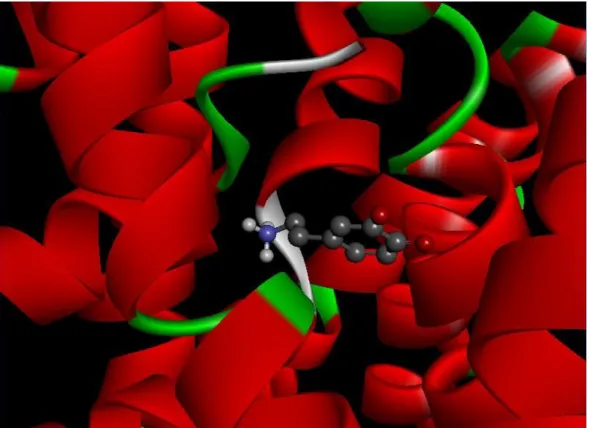
Figure 1.3 Crystal structure of LeuTAa, a bacterial homology of Na+/Cl- dependent neurotransmitter transporters. The determination of the X-ray structure of LeuTAa in complex with its substrate leucine and two Na ions (PDB entry of 2A65 at 1.65 A resolution) has been viewed as a milestone in understanding structural and functional relationships of NSS members. Figure 1.4 Shows model of human DAT with dopamine. Red bars indicate alpha

helices and dopamine shown in ball-and-stick.

Figure 2.1 Summary of PAM and BLOSUM matrices. High-value BLOSUM matrices and low-value PAM matrices are best suited to study well- conserved proteins such as mouse and rat RBP. BLOSUM matrices

with low number (e.g.; BLOSUM45) or high PAM numbers are best suited to detect distantly related proteins.

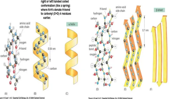
Figure 2.2 Polypeptide chains often fold into one of two orderly repeating forms known as the α helix and the β sheet.

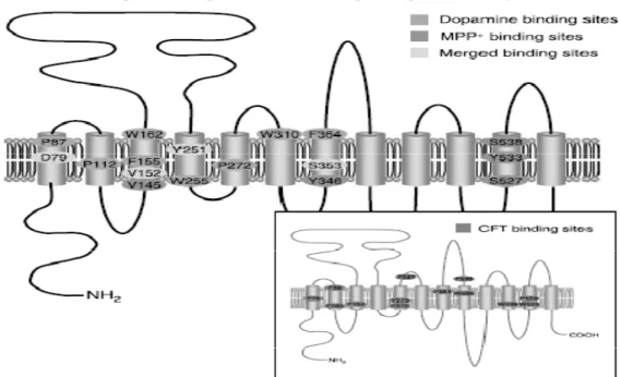
Figure 2.3 Putative topology and structural features of the DAT protein.

Figure 2.4 First picture, shows a target structure superposed on a template structure. Second picture, shows only the target model with the end of the core regions where an insertion has to be modeled.

(13)

xi

Figure 2.5 A schematic illustration viewing the database search method for building loop.

Figure 2.6 (A) In cases where the side chains at a given position are identical, the conformation of the target side chain can be extracted directly from the template. (B) In cases where the side chains are similar but not identical, most of the target side chain can be built from the template. (C) In cases where the side chains are different, the conformation of the target side chain has to be deduced from a library of rotamer structures and an assessment of the energetic.

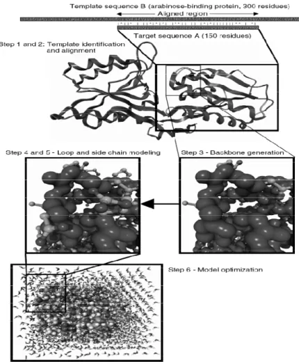
Figure 2.7 Steps in homology modeling. Example, the fragment of the template (arabinose-binding protein) corresponding to the region aligned with the target sequence forms the basis of the model (including conserved side chains). Loops and missing side chains are predicted, then the model is optimized (in this case together with surrounding water molecules).

Figure 3.1 Schematic illustration of a matching algorithm (a) and genetic algorithm (b) in the context of docking of a flexible ligand.

Figure 4.1 Sequence alignment results from BLAST. Blue: identical alignment similarity, light blue: weak alignment similarity, dark blue: strong alignment similarity.

Figure 4.2 The map view displays the coverage of the hits in a map, with one line per sequence. The bars are colored according to the bit score of the hits (with above 400, red, being the best hits).

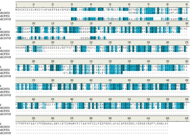
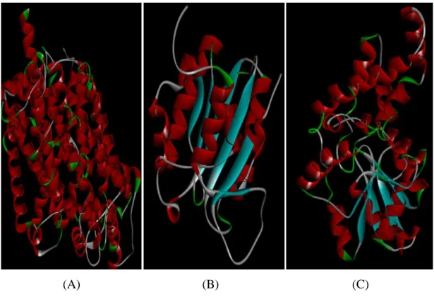
Figure 4.3 The sequence alignment analysis pertaining to the template (2A65, 3FZEA, 1SWWB) and the model (gi: human DAT) proteins. According to the secondary structure definition of Kabsch and Sanger, alpha helix regions are shown in orange. The parts of the model protein and the template proteins which haven't been aligned are defined as X. Figure 4.4 Template structures: 2A65(A); 3FZEA(B); 1SWWB(C). Red bars

indicate alpha helices, blue arrows indicate beta strands and green arrows indicate coil.

(14)

xii

Figure 4.5 The structure alignment results of the models (gi: hDAT), templates (2A65A, 3FZEA, 1SWWB) and the model proteins (gi.M0001 and gi.M0002) created through the MODELER program. Regions colored in orange represent the alpha helix and the arrows colored in blue represent the beta-sheets.

Figure 4.6 The resultant 3D model structures of giM0001 (A) and giM0002 (B). Red bars indicate alpha helices and green arrows indicate coil.

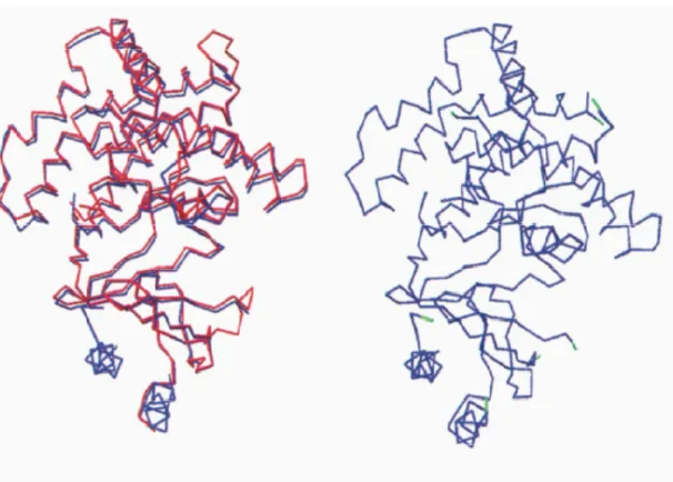
Figure 4.7 The superimposed poses of the tertiary structure prediction result for giM0002 (model protein) from MODELER and the 3D structure of template protein 2A65 from two different view. Yellow color: giM0002 red color: 2A65.

Figure 4.8 The 3D structure of the hDAT protein after the energy minimisation. Purple represents the alpha helix, blue represents the helix_3_10, green represents the turn and red represents sodium ions.

Figure 4.9 Nucleic acid and deduced amino acid sequences of the hDAT cDNA clone. The 12 TMH domains are boxed.

Figure 4.10 Sequence alignment results from BLAST. For BLAST searches; hDAT (query sequence) are aligned with the rDAT_robetta sequence. Figure 4.11 3D structure of rDAT_robetta (A), model structure giM0001 (B) and

giM0002 (C).

Figure 4.12 The tertiary structure prediction results rDAT (template protein) red color and giM0001 (model protein) yellow color.

Figure 4.13 The hDAT model structure (red) created instially by using multiple templates from the database and the hDAT model structure (blue) created as the second which based on the rDAT_robetta as a template. Figure 5.1 Structures of the eight ligands studie as the DAT receptor.

5-hydroxydopamine(1), 6-hydroxydopamine(2), Dopamine(3), Amphetamine(4), Methamphetamine(5), Cocaine(6), Benzene-1.3-diol(benzenediol)(7), Tyramine(8).

Figure 5.2 (A) The structural energy minimized model of the 3D hDAT protein which has been obtained using multiple experimental data as template. (B) The structural model of the 3D hDAT created by taking the rDAT_robetta protein as template. (C) The 3D structural model pertaining to the rDAT_robetta protein.

(15)

xiii

Figure 5.3 Binding site regions pertaining to the hDAT_MS-ligand complexes. Protein is shown in line, and ligands are shown in CPK representation. Orange color cocaine, white color methamphetamine, purple color 5-hyroxydopamine, yellow color benzenediol, red color tyramine, green color amphetamine, blue color 6-hyroxydopamine and pink color dopamine.

Figure 5.4 Binding site regions pertaining to the hDAT_robetta-ligand complexes Protein is shown in line, ligands are shown in CPK. Orange color cocaine, white color methamphetamine, black color 5-hyroxydopamine, yellow color benzenediol, red color tyramine, green color amphetamine, blue color 6-hyroxydopamine and pink color dopamine.

Figure 5.5 Binding site regions pertaining to the rDAT_robetta-ligand complexes Protein is shown in line, ligands are shown in CPK. Orange color cocaine, white color methamphetamine, black color 5-hyroxydopamine, yellow color benzenediol, red color tyramine, green color amphetamine, blue color 6-hyroxydopamine and pink color dopamine.

Figure 5.6 Molecular interactions between hDAT_robetta and dopamine (A) and hDAT_robetta and cocaine (B) in their binding sites. Dopamine and Cocaine are shown in ball-and-stick and protein in lines.

Figure 5.7 Molecular interactions between rDAT_robetta and dopamine (A) and rDAT_robetta and cocaine (B). Dopamine and Cocaine are shown in ball-and-stick and protein in lines.

Figure 5.8 Binding regions of cocaine on the surface of rDAT_robetta. The rat DAT protein, rDAT_robetta indicated surf opaque surface and cocaine indicated with CPK representation.

Figure 5.9 Binding regions pertaining to hDAT_robetta-cocaine. hDAT_robetta indicated as transparent and cocaine indicated as VDW.

Figure 5.10 2D representation of the atomic interactions between the hDAT_MS-Tyramine . hDAT_MS-Tyramine is shown with ball-and-stick model.

Figure 5.11 3D representation of the atomic interactions between the hDAT_MS-Tyramine . hDAT_MS-Tyramine is shown in ball-and-stick model.

(16)

xiv

Figure 5.12 2D representation of the atomic interactions between the hDAT_robetta-Benz-1,3-diol. Benz-1,3-diol is shown in ball-and-stick model.

Figure 5.13 3D representation of the atomic interactions between the hDAT_robetta-Benz-1,3-diol. Benz-1,3-diol is shown in ball-and-stick model.

Figure 5.14 2D representation of the atomic interactions between the rDAT_robetta-Amphetamine. Amphetamine is shown in ball-and-stick model.

Figure 5.15 3D representation of the atomic interactions between the rDAT_robetta-amphetamine. Amphetamine is shown in ball-and-stick model.

(17)

xv

List of Symbols

ΔGbind: Estimation of Binding Affinity

m: sequence of length n: sequence of length m+1: the matrix dimension n+1: the matrix dimension

S(i,j): score

i-1: the score from the cell at position j-1: the score from the cell at position s[i,j]: the new score at position s[i,j-1]: the score one cell to the left

s[i-1,j]: the score immediately above the new cell K,λ: constants

m: length of query sequence n: length of the entire database S: score of the alignment E: expect value

Ki: binding constant V: pair-wise evaluations

: probability density function

: the single body distribution function for atom I and is a constant for a given protein

ΔSconf: entropy lost upon binding L: ligand

(18)

xvi

List of Abbreviations

STS: Ion-coupled secondary transporters superfamily NSS: Sodium symporter

DAT: Dopamine transporter GABA: Gama-aminobutyric acid DA: Dopamine

MPP: 1-methly-4-phenylpyridinium MD: Molecular Dynamics

LeuTAa: Leucine transpoter LacY: Lac permease

SERT: Serotonin transporter NET: Noradrenalin transporter 3D: Three dimension

NMR: Nuclear magnetic resonance hDAT: Human dopamine transporter BLAST: Basic local alignment search

BLOSUM: Blocks of aminoacid substitution matrix TM: Transmembrane

TMH: Transmembrane helix

DSSP: Dictionary of Protein Secondary Structure DOPE: Discrete Optimized Protein Energy PDF: Probability Density Function

PDB: Protein data bank

RMSD: Root-mean-square deviation MC: Monte carlo

GA: Genetic algorithm FF: Force field

SFs: Scoring functions PD: Parkinson

(19)

xvii SN: Substantia nigra

NM: Neuromelamin

GlpT: Glycerol-3-phosphate transporters DS: Discovery studio

gi: Query sequence E: Expect value

TMH: Transmembrane helix rDAT: rat dopamine transporter gpf: Grid parameter file

dpf: Docking parameter file MC: Monte Carlo

(20)

1

Chapter 1 Introduction

The focus of my thesis is the development and application of structure and function prediction methods on membrane proteins called the dopamine transporter (DAT) belonging to the ion-coupled secondary transporters superfamily (STS), taking place in a neurotransmitter sodium symporter (NSS) family [1].

Dopamine neurotransmitter is fundamental for cellular signalling processes that are responsible for information transfer in neurons functioning in the nervous system [2]. The DAT pertains to a large family of Na+ and Cl- dependent transporters. This family comprises other monoamine transporters, such as the norepinephrine and serotonin transporters, gama-aminobutyric acid (GABA) and glycine carriers [3].

There are some experimental studies performed on DAT to gain information about the working mechanism of it. And it has been proven through pharmacological studies that dopamine transporting by DAT is Na+/Cl- dependent [1]. The transport process of the DAT includes the translocation of the substrate dopamine (DA) and two sodium, one chloride ions across the cell membrane [4]. The uptake is energetically coupled to transmembrane concentration gradient of Na+, which is maintained by Na+ K+ ATPase [5].

(21)

2

Figure 1.1: Model for Na+ effects on the interaction of dopamine with its transporter in intact cell [6].

Furthermore, some other experimental studies show that the dopamine transporter ensures the return of dopamine into neurons and is a major target for a variety of pharmacologically active drugs and environmental toxins. Various substances, such as the psychostimulant amphetamine, the dopaminergic neurotoxin 1-methly-4-phenylpyridinium (MPP+) and several sympathomimetic amines, are structurally similar to dopamine. Therefore, they make up substrates for the dopamine carrier and can be transported. In addition to this, the dopamine transporter constitutes an important molecular target for the addictive drug cocaine and to some extent, antidepressants [2].

Figure 1.2: Mechanism of Cocaine and Amphetamine based DAT block: Cocaine binds DAT and slows transport and Amphetamine induces MAPK/PKC to phosphorylate DAT. Phosphorylation slows transport and triggers internalization of DAT [7].

(22)

3

Some more substantial experimental and computational studies, such as Zn2+ binding site engineering, site-directed mutagenesis, Molecular Dynamics (MD) simulations, have also been performed so far in order to further investigate the structure and potential mechanism of DAT [8].

The first structural study related to DAT is the x-ray crystal structure determination for a bacterial homolog of DAT, which is bacterial leucine transporter (LeuTAa) from NSS family. This bacterial homolog has recently been identified as

Aquifex aeolicus as a complex of substrate leucine and two sodium ions (PDB entry

of 2A65 at 1.65 A° resolution) [10].

Consequently, initial computational studies for the structure determination of human DAT (hDAT) had been based on the above LeuTAa template [1]. And some more computational studies make use of Na+/H+ antiporter or Lac permease (LacY) as the template [1]. Further molecular modelling studies had been performed on DAT, serotonin transporter (SERT), and noradrenalin transporter (NET) [1].

However, for the latter there is no experimental evidence supporting the previously reported models from any kind of structural or biological studies. Therefore, the structural models of DAT, SERT, and NET that have previously been reported are not good enough to be used for studying molecular interaction of psychotropic drugs with these transporters. Since, these structural models are not appropriate for the homology modelling of any member of the NSS family consequently, the predicted atomic interactions are not reliable as well.

Up to now, LeuTAa, which has similar structural folding and physiological features as other NSS family members, had been reported to be the most reasonable template to study the substrate binding and transporting mechanism for NSS transporters, especially for DAT and SERT [1].

(23)

4

Figure 1.3: Crystal structure of LeuTAa, a bacterial homology of Na+/Cl- dependent neurotransmitter transporters. The determination of the X-ray structure of LeuTAa in complex with its substrate leucine and two Na ions (PDB entry of 2A65 at 1.65 A° resolution) has been viewed as a milestone in understanding structural and functional relationships of NSS members [1].

As a result, even though there are several studies reported before, the structure and working mechanism of DAT is not revealed at the atomic scale. And furthermore, since the previous studies reported to be not enough, either because of the template they have used or the resolution of the experimental studies. In this thesis, new three-dimensional (3D) structural model of hDAT has been constructed through two different methods; first template is based on an experimental structure obtained from the protein database by the means of the multiple sequence alignment, whereas the second template protein was the protein DAT of rat. Following the construction of the 3D structure, two different hDAT models have been used to dock DAT ligands with automatic computational docking.

(24)

5

Figure 1.4: Shows model of human DAT with dopamine. Red bars indicate alpha helices and dopamine shown in ball-and-stick.

In the Chapter 2, we have given the basic theory of the homology modelling. Here we gave a brief theory of how to perform pairwise and multiple sequence alignment. Furthermore, we introduce the algorithms used for these sequence alignment; methodologies, which have two main categories as local and global alignment algorithms. Finally, in these two sections we talk about secondary structure from sequence and homology modelling of the protein structure. And in Chapter 3, we have given the theory of protein-ligand interaction which have two main categories as docking algorithm and scoring function.

In Chapter 4, we introduce the methods that we used to predict the 3D structural model of DAT. This model has been constructed through comparative homology modelling based on the most reasonable template proteins. At the end, we obtained two different hDAT.

And in Chapter 5, upon obtaining a 3D hDAT model, eight ligands that couple with the macromolecule have been docked using the AutoDock program to obtain the conformation and orientations for hDAT functional analysis. There are eight

(25)

6

ligand molecules, namely 5-hydroxydopamine, 6-hydroxydopamine, Dopamine, Amphetamine, Methamphetamine, Cocaine, Benzene-1.3-diol (benzenediol), Tyramine. These ligand molecules were tested on the predicted hDAT structure model.

(26)

7

Chapter 2 Theory of Homology Modelling

2.1 Introduction

Despite the newly developed techniques in molecular biology that allow rapid identification, isolation, sequencing of genes and consequently the sequences of many proteins, the task of acquiring the 3D structures of these proteins remains a time-consuming task. The 3D structure of the protein, along with the sequence, can provide us a detailed understanding of the protein's function, mechanism of action and its structure-function relation. As the main purpose of structural biology is to infer the three-dimensional structure through the sequence, different approaches are being taken in order to achieve this goal by making up for the constraints related to X-ray diffraction or Nuclear Magnetic Resonance (NMR).

In the field of computational biology there are several studies conducted to support the tertiary protein structure. The most important topic of these studies is the homology modelling method. The observation that tertiary structure is better conserved than amino acid sequence underlies this method of homology modelling [11]. This modelling enables us to detect common structural properties and especially the overall fold of proteins which have observable resemblance despite the considerable change they have undergone in the sequence. While obtaining experimental structures through methods such as X-ray crystallography and protein NMR requires a considerable amount of time and effort, homology modelling provides useful structural models for developing theories on a protein's function and directing prospective experimental work.

(27)

8

For building the first homology models wire and plastic models of bonds and atoms were used in the 1960s. Following this advancement, the first homology model structure, which was of the small globular protein α-lactalbumin, got published in 1968. Hen egg white lysozyme had been taken as the template protein of this model structure. Subsequently, X-ray crystallography method has shown that the model was basically precise except for the misconception that the structure of carboxy-terminal end is similar to that of lysozyme [12].

Basically, there are two types of methods that are used most frequently for tertiary structure prediction. The first is the homology modelling (also known as comparative or knowledge-based modelling) which functions on the basis of modelling the structure of an unknown protein with regard to the known structure of homologous protein. The other approach, which is known as threading of fold recognition, eliminates the need for a homologous protein structure because it tries to match the sequence with all known protein folds to identify the best fit [12].

In our thesis, we have predicted the three-dimensional structure of the human dopamine transporter (hDAT) protein by making use of the homology modelling methods. In the course of this research, we obtained two different 3D hDAT protein structures using two different homology modelling methods. Whereas the templates of the first modelling method were experimental structures, the template of the second method was a structure of the rat DAT protein.

Modelling process of a protein's three-dimensional structure consists of a few steps. Accordingly, this chapter is outlined as follows; first, an introductory information is given about sequence alignment methods, which are basically pairwise sequence alignment and multiple sequence alignment. Then, the algorithms used are explained as; local alignment and global alignment. After that, theory of the corresponding computational tools, i.e. BLAST and FASTA, are given. Definition of substitution matrices and scoring functions; which are PAM and BLOSUM, is included. Secondly, a description of the methods used for secondary structure prediction and structure assignment is given. Finally, principle of homology modelling with automatic homology modelling systems are explained.

(28)

9 2.1.1 Pairwise Sequence Alignment

Sequence alignments are intended to discover and illustrate the similarities, differences, or evolutionary relationships between sequences. Sequence alignment is generally divided into two category; global and local alignment. And for both global and local alignment methods there exists algorithms for performing pairwise

alignments, that is, the alignment of just two sequences, and for performing multiple sequence alignments, in which more than two sequences are aligned with each other

[13].

Pairwise sequence alignment methods are used to find the best-matching piecewise local or global alignments of two query sequences [13], where as in the multiple sequence alignment multiple data within databases are considered.

In this chapter, we will present the basic sequence alignment algorithms, broadly characterized as global alignment, semiglobal alignment, and local

alignment, which are also common in multiple sequence alignment.

2.1.2 Multiple Sequence Alignment

Though the alignment of all sequences together, instead of making use of a generalized representation of the sequence family, multiple sequence alignments are more effective for the comparison of similar sequences. In the cases where there are subgroups of sequences with mutual extra features that are not available in the complete sequences set, these features may disappear during the creation of a profile. This occurs when the subgroup can be used for generating a new profile which is used in the search for other sequences [12].

Multiple alignment programs such as ClustalW and T-Coffee execute Needleman-Wunsch global alignment for every pair of sequence and obtain from these alignments the measure used in developing the guide tree. This measure is, in fact, the evolutionary distance which is a measure of dissimilarity. The percentage of alignment sites at which various residues have been aligned is considered as the simplest evolutionary distance measure. The Needleman-Wunsch alignment of all

(29)

10

sequence pairs takes a very long time when there are too many sequences to be aligned. As a result, faster but more approximate methods have been suggested for obtaining a distance measure [12].

2.1.3 Algorithm of Sequence Alignment

There are two main types of alignment: global and local. The local alignment algorithm of Smith and Waterman (1981) is the most rigorous method by which subsets of two protein or DNA sequences can be aligned. A global alignment such as the method of Needleman and Wunsch (1970) contains the entire sequence of each protein or DNA sequence. At the sequence alignment stage of our research, we made use of the BLAST server which functions on the basis of the below mentioned algorithms [14].

2.1.3.1 Local Alignment Algorithm

Local alignment is extremely useful in a variety of applications such as database searching where we may wish to align domains of proteins.

For the Smith-Waterman algorithm a matrix is constructed with an extra row along the top and the extra column on the left side. Thus for sequences of lengths m and n, the matrix has dimensions m + 1 and n + 1. The score in each cell is selected as the maximum of the preceding diagonal or the score obtained from the introduction of a gap. However, the score cannot be negative: A rule introduced by Smith-Waterman algorithm is that if all other score options produce a negative value, then a zero must be inserted in the cell. Thus the score S(i,j) is given as the maximum of four possible values

1. The score from the cell at position i-1, j-1; that is, the score diagonally up to the left. To this score, add the new score at position s[i, j],which consists of either a match or a mismatch.

2. s(i, j-1)(i.e.,the score one cell to the left)minus a gap penalty

(30)

11

4. The number zero. This condition assures that there are no negative values in the matrix. In contrast negative numbers commonly occur in global alignments because of gap or mismatch penalties [14].

BLAST (Basic Local Alignment Search)

Having primarily been designed as a local alignment search tool, BLAST identifies alignments between a query sequence and database without the introduction of gaps. The current version of BLAST allows gaps in the alignment [14].

By making use of BLAST, the user can select one sequence (termed as the “query”) and furthermore achieve pairwise sequence alignments between the query and the whole database (termed the “target”). As a result BLAST returns just the closest matches of millions of alignments which are analysed in a BLAST search. It also enables you to compare query sequence to DNA or protein sequences in a database.

This algorithm can be described in three phases

1. BLAST compiles a preliminary list of pairwise alignment, called word pairs. 2. The algorithm scans a database for word pairs that meet some threshold score

T.

3. BLAST extends the word pairs to find those that surpass a cut-off score S, at which point those hits will be reported to the user. Scores are calculated from scoring (substitution) matrices (such as BLOSUM62) along with gap penalties [14].

Optional BLAST Search Parameters

We will initially focus our attention on a standard protein-protein BLAST search.

(31)

12

Scoring Matrix: Five amino acid substitution matrices are available for blastp protein-protein searches: PAM30, PAM70, BLOSUM45, BLOSUM62 (default), and BLOSUM80.

Gap Penalties: A gap is a space introduced into an alignment to compensate for insertions and deletions in one sequence relative to another.

Expect Threshold: A threshold value T is established as a cut-off for the score of aligned words. It can be lowered to identify more initial pairwise alignments. This will increase the time required to perform the search but may increase the sensitivity. The default setting for expect value threshold is 10 for blastn, blastp, blastx and tblastn.

Filter Low-Complexity: Low-complexity sequences are defined as having commonly found stretches of amino acids (or nucleotides) with limited information content.

Word Size: For protein searches, a window size of 3 (default) or 2 may be set. When a query is used to search a database, the BLAST algorithm first divides the query into a series of smaller sequences (words) of a particular length (word size), as will be described below

Expect value: Altschul and colleagues revised the application of extreme value distribution to BLAST. The following formula defines the distribution of function scores for two random sequences m and n.

E=K x m x n x e-λS

K,λ: constants

m: length of query sequence n: length of the entire database S: score of the alignment

(32)

13

E is the expect value of different alignment with the same or greater scores than some scores that are expected to be the results of a database search. Very small E-values of 10ˉ20 or less are usually collected from closely related sequences and these scores manifest the resemblance of the database and query sequences. The fact that the E-value is determined by the sequence length, the number of sequences in the database and the alignment score should always be kept in mind. A small E-value mostly signifies a better alignment. Likewise, a higher percentage identity implies a more accurate assessment of the importance of the resemblance between the database sequence and query sequence [14].

2.1.3.2 Global Alignment Algorithm

This algorithm is important because it produces an optimal alignment of protein or DNA sequences, even allowing the introduction of gaps.

We can describe the Needleman-Wunsch approach for global sequence alignment in three steps [14]:

1. Setting up a matrix 2. Scoring the matrix

3. Identifying the optimal alignment

The algorithms for two commonly used search programs BLAST and FASTA. They make use of indexing techniques such as suffix trees and hashing to locate short stretches of database sequences highly similar or identical to parts of the query sequence [14].

2.1.4 Substitution Matrices and Scoring

Referring to a substitution matrix, score values for all possible pairs of residue are calculated for the aligned pairs of amino acids. Among different types of substitution matrices used over the years, there were some based on theoretical considerations, such as the number of mutations that are necessary for converting one amino acid into another, or resemblances in physicochemical characteristics.

(33)

14

Nevertheless, the most effective matrices, which are based on analysis of alignments of many homologs of well-studied protein from a wide range of species, use real proof of what happened during evolution [12].

Two methods have been used in deriving substitution matrices from multiple sequence alignments and the resultant substitution matrices PAM and BLOSUM are used for calculating the scoring matrices [12].

The matrices of BLOSUM (Blocks of Amino Acid SUbstitution Matrix), which is a substitution matrix serving for protein sequence alignment, are based on local alignments and used for scoring alignments between evolutionarily variant protein sequences. First, BLOCKS database has been scanned for highly preserved regions of protein families (the ones without gaps in the sequence alignment) and relevant amino acid frequencies and their substitution probabilities have been calculated. Secondly, a log-odds score for 210 probable substitutions of the 20 standard amino acids has been computed. BLOSUM matrices, which are not extrapolated from related proteins as in the PAM Matrices, function on the basis of examined alignments [15].

Henikoff and Henikoff (1992,1996) used the BLOCKS database, which consisted of over 500 groups of local multiple alignments (blocks) of distantly related protein sequences. Thus the Henikoff’s focused on conserved regions (blocks) of proteins that are distantly related to each other [13].

The aptitude of a range of BLOSUM and PAM matrices was put to test by Henikoff and Henikoff (1992) in order to identify proteins in BLAST searches of database. BLOSUM 62's performance at identifying a variety of proteins was found to be slightly better than BLOSUM 60 or BLOSUM70; but much better than PAM matrices. Their matrices were particularly effective for determining weakly scoring alignments. Other scoring matrices in common used in BLAST searches are BLOSUM 50 (matrix that is best for the alignment of two proteins sharing about 50% identity) and BLOSUM90 [14].

(34)

15

Figure 2.1: Summary of PAM and BLOSUM matrices. High-value BLOSUM matrices and low-value PAM matrices are best suited to study well-conserved proteins such as mouse and rat RBP. BLOSUM matrices with low number (e.g.; BLOSUM45) or high PAM numbers are best suited to detect distantly related proteins.

As seen in the Figure 2.1, based on data from the alignment of highly linked protein families, PAM matrices contain the presumption that substitution probabilities for closely related proteins (e.g., PAM10) can be extrapolated to probabilities for distantly related proteins (e.g., PAM250). On the other hand, BLOSUM matrices are based on empirical observations of more distantly related protein alignments.

Considering all the properties of the substitution matrices, in our research, we preferred to use BLOSUM62 matrix as the scoring matrix [14].

2.2 Secondary structure from sequence

In the case of an atomic-resolution of a structure, the hydrogen bonds of the biopolymer define its secondary structure. In proteins, the patterns of hydrogen bonds between backbone amide and carboxyl groups identify the secondary structure. Whereas, in nucleic acids, it is the hydrogen bonding between the nitrogenous bases that identifies the secondary structure.

An α-helix is generated when a single polypeptide chain turns around itself to form a structurally rigid cylinder. A hydrogen bond is made between every fourth amino acid, linking the C=O of one peptide bond to the N-H of another. This gives rise to a regular helix with a complete turn every 3.6 amino acids [16].

(35)

16

β-strands (sheet) are created when hydrogen bonds form between segments of polypeptide chains lying side by side. A beta strand (also β strand) is a stretch of polypeptide chain typically 3 to 10 amino acid long with backbone in an almost fully extended conformation. When the structure consists of neighbouring polypeptide chains that run in the same orientation, it is considered a parallel β-sheet; opposite to that of its immediate neighbours-the structure is an antiparallel β-sheet [16].

Figure 2.2: Polypeptide chains often fold into one of two orderly repeating forms known as the α helix and the β sheet.

Most transmembrane (TM) proteins span the membrane in the form of one or more α-helix, and we shall discuss these first. The properties of the lipid bilayer force a number of structural constraints on the α-helical TM segments. An average membrane thickness is 30 Ao, which corresponds to an α-helix of between 15 and 30 residue [12].

(36)

17

Figure 2.3: Putative topology and structural features of the DAT protein.

DAT protein structure shown in the Figure 2.3. human dopamine transporter (hDAT), which is in the content of our thesis, pertains to NSS family. Results obtained from structure analysis of previous studies indicate that DAT pertaining to NSS family are transmembrane proteins with the following characteristics; 12 TM α-helices with intracellular location of N-terminal and C-terminal, and a large internal substrate binding cavity on the midpoint of the membrane [17].

Methods for predicting protein secondary structure can be broadly divided into the following categories: statistical analysis, also referred to as probabilistic analysis; knowledge-based analysis; machine-learning methods; and those mainly based on neural networks. Most automated methods in use today use a mixture of these techniques, and all of them incorporate some form of statistical analysis, is employed in most of the automated methods [12].

Many prediction programs are designed to recognize just three different regular structural states: α-helices, β-strand, and β-turns. There are also some algorithms that even try to predict different kinds of helical or turn conformations, such a -helices, 310-helices, and polyproline helices, and type I, II and other types of turns [12].

(37)

18

The most widely used of these programs is Dictionary of Protein Secondary Structure (DSSP), which assigns secondary structure according to hydrogen-bond patterns. DSSP, proposed by Wolfgang Kabsch and Chris Sander in 1983, takes the approach just described to assign helices.

Another program, STRIDE, uses both hydrogen-bond energy and backbone dihedral angles. DEFINE matches the interatomic distances in the protein with those from idealized secondary structures. However, these programs do not always produce identical results from the same data, giving slightly different secondary structure assignments. The differences are almost exclusively at the ends of structural elements. These differences in defining secondary structure elements can affect the apparent accuracy of secondary structure prediction methods. A prediction method should be trained and subsequently tested using training and testing datasets whose structural features were defined using the same assignment method [12].

Table 2.1: The eight structural states detailed by the DSSP method, with their descriptions.

DSSP, is commonly used to describe the protein secondary structure with single letter codes. There are eight types of secondary structure that DSSP defines:

· G = 3-turn helix (310 helix). Min length 3 residues.

· H = 4-turn helix (α helix). Min length 4 residues. · I = 5-turn helix (π helix). Min length 5 residues. · T = hydrogen bonded turn (β-turn)

· E = extended strand in parallel and/or anti-parallel β-strand conformation. Min length 2 residues.

· B = residue in isolated β-bridge (single pair β-sheet hydrogen bond formation) · S = bend (the only non-hydrogen-bond based assignment).

(38)

19 2.3 Homology modelling of protein structure

Homology modelling has several steps. The first step consists of finding structural homologues to the target protein. Most experimentally resolved structures are placed in the Protein Data Bank (PDB). Using one of the sequence-search programs (BLAST and FASTA), a database with the sequences of the PDB structures is searched with the target sequence for homologues. The protein with the highest similarity score and highest sequence identity over the largest stretch of amino acids is chosen as the template. Having identified a matching template protein, the next step should be the alignment of the target and template sequences. The most important step in the modelling process is this alignment [12]. After alignment, the structurally conserved regions-the core-are modelled first. Modelling the core is simply achieved by transferring the x, y, and z coordinates of every matched atom within an aligned residue from the template to the target molecule. The backbone atoms are then joined together to form peptide bonds at the correct angles. It is usually possible to copy only some of the side-chain coordinates, as many side chains in the target will not be identical to those in the template. Regions with insertions and deletions are left for later. It is important to check the core for misfits. In regions that were difficult to align, one should examine whether the insertion by one or two residues would position it in a more favourable conformation [12].

(39)

20

Figure 2.4: First picture, shows a target structure superposed on a template structure. Second picture, shows only the target model with the end of the core regions where an insertion has to be modelled [12].

Once a good alignment has been obtained, the other major procedure in model building is modelling the loops. These are the regions that usually contain insertions or deletions and the most variable in sequence. Because of their variability in both sequence and length, loops are generally the most difficult regions to model. If the target protein contains an insertion in a loop sequence relative to the template structure, there will be no template coordinates from which to model the insertion. The easiest way round this problem is if there are other structure homologs with the same insertion. It is then possible to model the missing part using their coordinates. However, an insertion is often unique to the target protein. In this case, the most widely used method for modelling loops, in both manual and automatic procedures, is to search for fragments of the same length in a database of high-resolution structures. Loops that have the lowest RMSD are selected for further evaluation [12].

(40)

21

Figure 2.5: A schematic illustration viewing the database search method for building loop [12].

Then, to be able to build side chains in a model, however, it is necessary to have some understanding of the conformations they can adopt. A study of atomic coordinates of side-chain atoms of conserved residues in proteins with similar three-dimensional structure has found that in more than 90% of cases the side chains have the same conformations in the two proteins. To predict the side-chain conformation when the aligned residues are not identical, rotamer libraries are used [12].

(41)

22

Figure 2.6: (A) In cases where the side chains at a given position are identical, the conformation of the target side chain can be extracted directly from the template. (B) In cases where the side chains are similar but not identical, most of the target side chain can be built from the template. (C) In cases where the side chains are different, the conformation of the target side chain has to be deduced from a library of rotamer structures and an assessment of the energetic [12].

And the final step is the model optimization. This method boils down to a sequence of rotamer prediction and energy minimization steps. At every minimization step, a few big errors (like bumps, i.e., too short atomic distances) are removed while many small errors are introduced. When the big errors are gone, the small ones start accumulating and the model moves away from the target. As a rule of thumb, today’s modelling programs therefore either restrain the atom positions and/or apply only a few hundred steps of energy minimization. In short, model optimization does not work until energy functions (force fields) get more precise. Such a simulation follows the motions of the protein on a femtosecond (10-15) timescale and mimics the true folding process [18].

(42)

23

Figure 2.7: Steps in homology modelling. Example, the fragment of the template (arabinose-binding protein) corresponding to the region aligned with the target sequence forms the basis of the model (including conserved side chains). Loops and missing side chains are predicted, then the model is optimized (in this case together with surrounding water molecules) [18].

2.3.1 Automated Homology Modelling

Having changed modelling into a practically routine technique for the observation of the three-dimensional structure of a new protein, automated model building by homology has revolutionized the modelling assignment. Fully automatic model-building programs, such as Swiss-Model and MODELLER, brought along the advantages of objectivity, rapidity. We made use of the MODELLER program for the homology modelling in our research. Information about this program is given below [12].

(43)

24 2.3.1.1 MODELLER

With the aim of satisfying constraints, MODELLER develops a hypothetical target structure based on a familiar template structure. First, these spatial constraints in the form of atom-atom distances and dihedral angles are extracted from the template(s), used in the target and afterwards synthesized with general rules of protein structure like bond length and angle preferences.

The alignment enables us to identify parallel residues between the target and the template. The optimization of the target model continues until a model that best satisfies the spatial constraints is obtained. MODELLER is most commonly used for homology modelling of protein's three-dimensional structure as the program deduces structure by satisfaction of spatial constraints; yet, it can also be put into use in experimental structure determination by NMR. The output of MODELLER is a tertiary structure of a protein that satisfies a set of constraints as well as possible [11].

MODELLER protocol evaluates protein structure using the Probability Density Function (PDF) energy data and DOPE (Discrete Optimized Protein Energy) scoring function (in the tutorial) [19].

PDF (Probability Density Function)

In order to constrain a model towards the structure of the template and to preserve fine structure geometry, MODELLER creates numerous restraints. There are dissatisfied restraints at the end of a MODELLER refinement and in order to obtain an evidence of the quality of the model for that particular residue, the PDF energy (i.e., the value of the objective function) regarding each residue is summed. As parts of a model (for example residues alongside an insertion or deletion) are practically sure to have higher restraint violations, a simple interpretation of the absolute value of the energy does not exist. The energies are effective for comparisons between different models. Models with lower energy in a given region are probably better in that region. If these models have been developed from different initial alignments of the model sequence and the homologues, then lower

(44)

25

energies are an evidence of better alignment. Either residue or atomic based statistical potentials are used as quality indicators of protein structures and as potential energy functions in predicting protein structures.

PDF Physical Energy is more of a true energy term. It is comprised of the sum

of energies for the stereo chemical pseudo-energy terms which consist of valence bonds, valence angles and torsion angles, improper torsion angles, and soft-sphere repulsion, as well as knowledge based non-bonded potentials used only for loop and mutant modelling. Higher energy indicates a larger restraint violation in the model.

PDF Total Energy is the total PDF energy, that is the sum of the scoring

function value of all homology-derived pseudo-energy terms and stereo chemical pseudo-energy terms.

DOPE Scoring Function

Many statistical potentials, either residue based or atomic based are used in evaluating the quality of protein structures and as potential energy functions in predicting protein structures.

DOPE is an atomic based statistical potential in MODELLER package for model evaluation and structure prediction. The DOPE score of a protein can be viewed as a conformational energy which measures the relative stability of conformation with respect to other conformations of the same protein. It can assist in choosing the best model out of a set of predicted model structures of a protein sequence. And low scores are better.

In addition, the statistical potential is also used as part of the energy function in predicting loop models or to optimize the local structure of a mutated residue.

The pairwise statistical potential function of a protein with N atoms can be represented by the pairwise probability density function:

(45)

26

3, .

:

where ₃ is the single body distribution function for atom i and is a constant for a given protein.

The pairwise probability density function is proportional to ₃ _. and the (m,n) pair density where m and n are the atom types of atom i and atom j respectively.

The density of (m,n) pairs at distance r is pmn(r)/(4πr2Δr). For a finite system, such as a protein structure, the spherical shell can be partly outside of the protein boundary in many cases and the density should be more accurately represented by pmn (r)/n(r,a) where n(r,a) = 4πr2ξ(r)

3, . 3 . ú /Hn 0

The scores used in the current MODELLER are calculated as a weighted sum from a set of high resolution X-ray structures with low sequence homology:

3, . 7 ,ú , /ú ,

For all the heavy atoms in the 20 standard amino acid residue types, MODELLER determines 158 various atom types. DOPE scores are calculated for each pair of heavy atoms, excluding the N-terminal nitrogen and C-terminal oxygen atoms and tabulated for distances from 0 to 15 Ao with an interval of 0.5 Ao. Atom pairs between different residues have the pair potential; however, the calculation does not include the atom pairs in bond, angle, and torsion angle.

Then, the scores are entered into the cubic spline function. This function not only calculates the single point energy of a protein model, but also calculates the first and second derivatives of the energy function in molecular dynamics protocol. A protein's absolute score is insignificant as the DOPE energy is not standardized

(46)

27

depending on the proportions of the protein. Nevertheless, in model assessment, the related energies of various conformations are effective. Single chain protein structures form a potential. Making use of the score on single chain proteins is highly secure.

DOPE scores can be calculated at high and regular resolutions; for former, a bin size of 0.125 and for latter, a bin size of 0.5 is needed.

2.3.1.2 Verify protein

Verify protein protocol is mostly used in the final phase of a homology modelling for analysing a preliminary protein structure on the basis of experimental data. Compatibility of a protein's structure with its own sequence is a requirement for the functioning of this protocol.

The strategy that Verify Protein makes use of comprises building a protein's 3D profile and calculating its compatibility with the same protein's sequence. Verify Protein can also be used to calculate local 3D-1D scores in a fixed-length sliding window (typically about 5 to 20 residues long). These can be plotted against residue position to expose local regions of comparatively high or low 3D-1D compatibility. Regions with remarkably low scores are likely to be places where the backbone has been incorrectly threaded through the electron density data (if the structure is experimental) [19].

(47)

28

Chapter 3 Prediction of protein-ligand interaction in drug design

3.1 Introduction

Due to the vital role they play in critical metabolic pathways and the incomparable opportunities they offer for structure-based drug design and discovery, many of the macromolecules are considered to be potential therapeutic targets. With a growing importance in the endeavour, structure-based design has now become an integral part of medicinal chemistry [20].

Relenza, which is used for the treatment of flu, is the first drug to be designed in that way. It was developed through the selection of molecules that had the potential of binding the conserved regions of the enzyme neuraminidase, which is created by the flu virus to take newly formed viruses away from infected cells. The prevention of this enzyme would therefore keep new viruses from being dispersed into the body. For the prevention of the parainfluenza virus hemaglutinin-neuraminidase, a similar structure-based approach was applied [12]. Experimental techniques and their outcomes in the database help computational drug design by providing the 3D structure of proteins. More than 35,000 crystallographic or NMR structures of proteins or nucleic acids are available in the Protein Data Bank (PDB). Furthermore, the rate of 3D macromolecular structure identification keeps increasing every year, especially with the development of new techniques such as X-ray crystallography [20]. The interest in computational methods continues to increase for the prediction of protein-drug docking.

When trying to find out the structure of a protein-ligand complex, a problem may sometimes occur in X-ray crystallography. Through analogy with previously

(48)

29

identified homologous proteins, the positions of the protein atoms can be identified more directly. However, the electron density of the ligand may occasionally turn out to be too unclear to determine the atomic positions of its binding mode. Identification of the most favourable conformation of the ligand when bound to the protein molecule can be achieved through computational docking. The protein molecule may later be tested for affinity with the experimental electron density [21].

Computational docking may be used to identify the most convenient form of the ligand when bound to the protein molecule, which may then be tested for compatibility with the experimental electron density. Likewise, making use of computation, the binding of substrates, products, and transition states may be predicted. This would also allow study of enzyme mechanisms and bound states which couldn't be studied experimentally [21].

The structural and energetic recognition of a ligand and a protein helps determine the selective binding of a low-molecular-weight ligand to a particular protein. Free energy decreases when a bond between atoms is formed. ΔG is thus negative. The binding affinity can be determined from the experimentally measured binding constant Ki

ΔG= –RT ln Kİ = ΔH-TΔS

The experimentally estimated binding constant Ki ranges mostly between 10-2 and 10-12 M, equal to a Gibbs free energy of binding ΔG between -10 and -70 kj/mol in aqueous solution [22]. Beside the experimental techniques used for the determination of ΔG, there are also computational methods for that. Docking is one of these methods. Docking protocols are considered to be a combination of a search algorithm and scoring functions. The number of various search algorithms and scoring functions is comparatively large and continues to increase. The degrees of freedom of the protein-ligand system should allow for the system to be adequately tested by the search algorithm, so that it consists of true binding modes. Speed and effectiveness in covering the related conformational space are certainly the key elements of a search algorithm. In addition to these essentials, the thermodynamics of interaction of the protein-ligand system should sufficiently be covered in the

(49)

30

scoring function in a way that the true binding modes could be separated from all the others discovered and be classified appropriately.

3.2Docking algorithm

In the prediction of a ligand binding pose, the effectiveness of a docking algorithm is usually evaluated in terms of the root-mean-square deviation (RMSD) between the experimentally observed heavy-atom positions of the ligands and the system is major challenge in the search for the correct pose. The number of degrees of freedom included in the conformational search is the main feature that affects the searching efficiency. Docking algorithm falls into two general categories: Flexible docking search algorithm and matching algorithm.

3.2.1 Flexible docking search algorithm

Flexible docking search algorithm three general categories of algorithms are designed to treat ligand flexibility: systematic methods; random or stochastic methods; and simulation methods [20].

The systematic search algorithms attempt to examine all the degrees of freedom in a molecule, and can be further divided in three main types: conformational search methods, fragmentation methods, and database methods.

Random search algorithms test the conformational space by performing random changes to a single ligand or multiple ligands. There are three main types of methods based on random algorithms: Monte Carlo methods (MC), Genetic Algorithm methods (GA), and Tabu Search methods [20].

Many programmes function on the basis of GAs (for example, AutoDock, DARWIN, DIVALI, GOLD, EADock, FITTED and PSI-DOCK) [23]. Genetic algorithms (GAs) benefit from ideas obtained from genetics and the theory of biological evolution to docking. GAs firstly start from a population of diverse conformations of the ligand regarding the protein. Each conformation is characterized by a set of state variables (described as genes) that describe facets such