VIVALDI ANTENNA DESIGN FOR GPR APPLICATION

T.C

ISTANBUL AYDIN UNIVERSITY

INSTITUTE OF SCIENCE AND TECHNOLOGY

VIVALDI ANTENNA DESIGN FOR GPR APPLICATION

THESIS

Bader AWAD

Department of Electrical and Electronics Engineering Electrical and Electronics Engineering Program

T.C

ISTANBUL AYDIN UNIVERSITY

INSTITUTE OF SCIENCE AND TECHNOLOGY

VIVALDI ANTENNA DESIGN FOR GPR APPLICATION

THESIS

Bader AWAD (Y1713.300013)

Department of Electrical and Electronics Engineering Electrical and Electronics Engineering Program

DECLARATION

At this moment I declare that all information in this thesis document has been obtained and presented in accordance with academic rules and ethnic conduct at Istanbul Aydin University. And I also declare that, as required by these rules and also ethnical conduct, I have fully citied and also referenced all material and results which are not original from this thesis.

FOREWORD

This thesis is about Designing antenna for GPR application. According to the thesis we introduced meaning of GPR, principle of GPR work, major area for using this technology, moreover our interest in the most important part of GPR application.

I started to study Electrical and Electronics Engineering in Bachelor degree, my passion to study this field comes from my love to analytical subjects like mathematics and physics and engagement in this two field.

During my study I attended a lot of courses in this field like Mobile Communications Radar Equations, wireless communication, Microwave theory and Antenna design. But, my interest was in studying Antenna and how this device work and the criteria that must be taken to design a good antenna according to work that interest in. The amount of researches fast paced development and the number of opportunity in this area grasped my interest and I decided to complete my Master Degree in this field.

When I joined to my Master Degree in Electrical and Electronics Engineering I started to take courses in Electrical Engineering but, I wanted to be my thesis in Antenna Design , after that I met Assoc. Prof. Dr. SAEID KARAMZADEH, in that time he advised me to study some subjects related to Antenna Design , one of those subjects was GPR . I began to collect information about the subject, what is the GPR?, how its work? what are the parts of the device? what type of antenna that will be used to design GPR? What is the simulation programs that I shall use that to design the antenna?

My experience in this work during one year started from knowing the principle of GPR and the fields which GPR work in. In additional to design the important factor to work this technology properly, that is the Antenna. After knowing the type of antenna I had to learn about some simulation programs related to antenna. So, I interested in two types of these simulations programs; Asis HFSS and CST.

Therefore, I started to design the required antenna (Vivaldi Antenna) after reading a lot of reference papers and literature reviews about the design and antennas characteristics. But during the work I faced some difficulties like to choose appropriate size, substrate material and frequency band, until to get the final designs.

Eventually, I would like to thank my advisor Assoc. Prof. Dr. SAEID KARAMZADEH and appreciate his efforts during our work for deeply advices and for his guidance, assistant and support.

And all thanks to my family.

TABLE OF CONTENT

Page

FOREWORD ... vii

TABLE OF CONTENT ... ix

ABBREVIATIONS. ... xi

LIST OF FIGURES ... xiii

LIST OF TABLES ... xv

ABSTRACT ... xvii

ÖZET ... xix

1. INTRUDUCTION ... 1

1.1 What is Ground Penetrating Radar? ... 1

1.2 GPR's Structure ... 1

1.2.1 Reflected signal ... 2

1.2.2 GPR Depth Determination ... 3

1.2.3 How deep can GPR go into ground? ... 3

1.3 Types of Ground Penetrating Radar ... 4

1.3.1 Impulse GPR ... 4

1.3.2 Continuous-Wave GPR ... 4

1.4 GPR Applications Area ... 5

1.5 Three _ Dimensional Imaging ... 5

2. ANTENNA ... 7

2.1 Definition ... 7

2.2 Radiation Pattern ... 7

2.2.1 Antenna pattern in 3D ... 7

2.2.2 Antenna Pattern in 2D ... 8

2.2.3 Antenna pattern lobes ... 8

2.3 Intensity of Radiation ... 9 2.4 Beamwidth ... 10 2.5 Directivity ... 10 2.6 Gain ... 12 2.7 Efficiency Of Antenna... 13 2.8 Input Impedance ... 16

2.9 Return Loss And S11_Parameter ... 17

3. ANTENNA TYPES ... 19

3.1 Wire Antenna ... 19

3.2 Microstrip Antenna ... 23

3.3 Aperture Antenna ... 29

4. METHODOLOGY AND RESULTS DISCUSSION ... 31

4.1 Antipodal Vivaldi Antenna (AVA). ... 31

4.2 Double Slot Antipodal Vivaldi Antenna (DSAVA). ... 37

4.3 CST Studio Suite ... 41

REFFERENCES... 45 RESUME ... 49

ABBREVIATIONS.

UWB : Ultra -wide Band

AVA : Antipodal Vivaldi Antenna GPR : Ground Penetrating Radar SAR : Synthetic- Aperture Radar EMW : Electromagnetic Wave

SFCW : Stepped-Frequency Continuous-Wave IF : Intermediate Frequency

RFI : Radio Frequency Interference HPBW : Half-power beamwidth FNBW : First-null beamwidth

dBi : Decibels relative to isotropic VSWR : Voltage Standing Wave Ratio

DSAVA : Double Slot Antipodal Vivaldi Antenna

HFSS : High Frequency Structure Simulator CST : Computer Simulation Technology AR : Axial Ratio

LIST OF FIGURES

Page

Figure 1.1: GPR working principle . ... 2

Figure 1.2: Radio wave penetrate the ground as elliptical cone. ... 2

Figure 1.3: Impulse GPR system block diagram ... 4

Figure 1.4: A: Chair display of the Miami Oolite 3D GPR survey ... 5

Figure 2.1: The 3D Antenna Radiation Pattern. ... 8

Figure 2.2: The one direction antenna pattern in V and H planes. V plane represents the Vertical pattern, where H plane represents the Horizontal pattern ... 8

Figure 2.3: (a) antenna pattern of radiation main lobe .(b) power pattern and radiation ... 9

Figure 2.4: the two dimensional power pattern... 10

Figure 2.5: Antenna beam Ω . (a) radiation intensity U from a real antenna . (b) intensity of the radiation with all radiation from the real antenna focused into a cone of solid angle Ω with constant intensity of the radiation equal to the maximum of the real pattern . ... 11

Figure2.6: Reference terminal and reference of antenna ... 14

Figure 2.7: Linear , Circular and Elliptical Polarization ... 14

Figure2.8: Radiation Pattern of a polarized circular test antenna given with a rotating, polarized linearly, antenna source. ... 15

Figure 2.9: Equivalent circuits of transmitting antenna ... 17

Figure 3.1: Dipole and monopole antenna (a) Dipole (b)monopole .. ... 19

Figure 3.2. current distribution for various different-fed dipoles ... 20

Figure 3.3: Feed point variations R a and reactance X ... 20

Figure 3.4: Infinitesimal dipole ... 21

Figure 3.5: Antenna pattern for an infinitesimal dipole . ... 21

Figure 3.6: Folded dipole antenna... 22

Figure 3.7: Log periodic dipole array(a)log periodic and (b) its equivalent . ... 22

Figure 3.8: A broadband dipole curtain ... 23

Figure 3.9: Yagi Uda array . ... 23

Figure 3.10: The rectangular patch microstrip antenna ... 24

Figure 3.11: the fields of the microstrip antenna at W=L=0.5 λ. ... 25

Figure 3.12: Helical antenna with ground plane . ... 26

Figure 3.13: Commercial helix ... 26

Figure 3.14: Design of helix. ... 27

Figure3.15: curve of the Equiangular spiral with r= and ... 28

Figure 3.16: Planar equiangular spiral antenna ... 28

Figure 3.17: Archimedean spiral antenna ... 28

Figure 3.18: Vivaldi Antenna ... 29

Figure 4.1: AVAs. (a) Typical AVA . (b) AVA with lens .(c) Proposed AVA. ... 32 Figure 4.2: Simulated gain. (a) Typical AVA ,AVA with lens and Proposed

Antenna.(b) Proposed AVA with different T Distance... 32 Figure 4.3: (a) Proposed AVA ,(b) Proposed AVA two slots ... 33 Figure 4.4: S11 simulations ,(a) Typical AVA, AVA with lens , Proposed AVA , (b) Proposed AVA at different T Distance. ... 34 Figure 4.5: simulation radiation pattern of the antenna . (a) 3GHz. (b) 8.9 GHz.

(c)15 GHz. ... 35 Figure 4.6: Antenna pattern of the antenna. (a)3 GHz . (b) 8.9 GHz . (c) 15 GHz. .. 36 Figure 4.7: configuration of DSAVA . (a) Typical DSAVA. (b) DSAVA with

elliptical shape . (c) Proposed DSAVA. ... 37 Figure 4.8: S11 simulations . Typical DSAVA , elliptical shape, cylinder shape and

Proposed DSAVA. ... 38 Figure 4.9: (a) Proposed DSAVA , (b) Proposed DSAVA two slots. ... 38 Figure 4.10: Kimulated gain. Typical DSAVA , elliptical shape , cylinder shape ,

Proposed DSAVA . ... 39 Figure 4.11: Simulation radiation pattern of the Proposed DSAVA (a) 4 GHz , (b)

9.05 GHz , (c) 15 GHz. ... 40 Figure 4.12: antenna pattern. (a) 3.55 GHz . (b) 9.05 GHz . (c) 15 GHz. ... 41 Figure 4.13: CST Studio 3D interactive modeling. ... 42

LIST OF TABLES

Page

Table 1.1: Dielectric constant for some materials. ... 3

Table 4.1: Proposed AVA Dimensions. ... 33

Table 4.2: Comparison of Antenna Characteristic and literature. ... 35

Table 4.3: Proposed DSAVA Dimensions. ... 39

VIVALDI ANTENNA DESIGN FOR GPR APPLICATION ABSTRACT

Ground Penetrating Radar (GPR) is a radar which detects objects and interfaces buried beneath the earth’s surface. It is considered as a very effective tool for non-destructively sensing of the subsurface environment, since the radar can detect any object that has different electrical properties than the surrounding soil. Thus it senses both metallic and nonmetallic targets as opposed to metal detectors. The GPR system usually contains a receiver and transmitter antennas. Transmitter connected with a source, and receiver connected with signal processing. Civil and military sections are the most popular areas for the GPR applications. In military area, it is commonly used for finding unexploded bombs, underground warehouses, bomb shelters, discovering enemy communication channels, secret rooms. In civil life GPR is commonly applied for finding, buried pipes and undetected voids. Together with these, GPR is used to find people behind the rubble also.

The antennas type is very important, so the antenna plays an important role in GPR systems. The antenna efficiency is also an important part of the system. The high efficiency provides reliable and more information. Having better antenna efficiency depends on the optimization works in antenna's physical features.

Therefore, Vivaldi antenna is one of UWB Antenna that used to build GPR , because it has some properties like great bandwidth , end-fire radiation, moderate gain , small dimension and easy to fabricate. So, in this thesis we have a plan to build two types of Vivaldi antenna one is Antipodal Vivaldi Antenna (AVA) and another Double Slot Vivaldi Antenna (DSAVA), for AVA the substrate material that used is Taconic with dielectric constant 3.55 we aim in this design to get a good antenna pattern at low frequencies and a high radiation pattern at high frequency , whereas it has a small dimension (70×50×0.76)mm3 . In DSAVA we have to get radiation pattern greater than that in AVA , because DSAVA is improved to enhance the Directivity and radiation pattern , the substrate material that used is FR4 with dielectric constant 4.3 and dimension 50×70×1 mm3 , in two designs we used the dielectric lens to improve the radiation pattern at low and high frequency , and for AVA we used a technique elliptical curved edge to enhance the return loss or S11 at low frequencies. Keywords: Double slot Antipodal Vivaldi Antenna (DSAVA), Antipodal Vivaldi

YERALTI GÖRÜNTELEME RADARI İÇİN VİVALDİ ANTEN TASARIMI ÖZET

Yeraltı Görünteleme Radarları (YGR) günümüzde birçok askeri ve sivil uygulamalarda kullanlımlaktadır. Askeri alanda, gömülü nesne, mayın ve patlayıcı tesbiti için önemli rol almaktadır. Sivil uygulamalarda ise, arkeologi çalışmalarında tarihi eserlerin hasarsız tesbiti, plastik ve metal boruların su sızıntılarını bulmak ve inşa edilmiş bir binanın iskelet yapısını incelemek için kullanılmaktadır. Bu radar çeşiti, sadece tesbit etmek değil, harek izleme yeteniğine de sahiptir. Bu doğrultuda insan hareketleri tesbiti de yapılmaktadır. Duvar arkasında saklanan insanlar, deprem sonrası enkaz altında kalmış ve kurtarmayı bekleyenlerın hayatını kurtarmak için, önemli bir teknoloji olarak sunulmuştur.

YGR teknolojisinin en önemli parçası olarak YGR anteni de geliştirilmekte olup, araştırmacılar için odak noktası olmuştur. Bu teknolojide anten tasarımı yaparken, antenin daha iyi ve eş zamanlı data alışverişini sağlamak için geniş bant genişlğine sahip olması, gönderilen işaretin daha derin mesafelere ulaşmak için yüksek kazanca ve başlangıç frekansının düşük olmasına özen gösterilmesi önerilmiştir. Ayrıca, tasırımı yapılacak olan antenin, alıcı verici sitemi ile beraber kullanılması gerektiği ve dron gibi araçlara monte edilebilmesi için oldukça hafif olup, küçük boyutlara sahip olması büyük bir avantaj sağlayacaktır.

Bu doğrultuda, tez çalışması esnasında, YGR sistemleri kapsamlı birşekilde araştırılıp, kullanılan anten yapıları incelenecektir. Anten tasarımına başmadan önce, antenin tüm parameteleri ve çeşitleri gözden geçirelecektir. Tasarım aşamasında ise, literatür araştırmasının ardından oldukç hafıf, küçük boyutlu, yüksek kazanca sahip ve ultra geniş bantlı Vivaldi anten tasarımı gerçekleştirilecektir.

1. INTRUDUCTION

1.1 What is Ground Penetrating Radar?

GPR (Ground Penetrating Radar) is the non-devasting device used to detect object or hidden materials underground by using a pulses of electromagnetics wave. The electromagnetic pulses will be reflected or diffracted when the dielectric constant of ground is variable [1], [2].

GPR is a non-devasting device, a GPR system transmits an electromagnetic pulses some these pulses reflected on the ground when the dielectric constant is varying the reflected pulses received by a receiver and then transmits to the control unit, in this unit the period of time between transmitting and receiving will calculated, in the display unit it appears the different material [3].

1.2 GPR's Structure

GPR, includes a data collection device, transmitter, and a receiver (digital recorder or analog printer). The transmitting antenna transmits wave of electromagnetic to the ground, after that a sensor detects the wave that reflected from the surface. the radar paly to transmits wave after that the receiver receive the reflected wave on the surface, the control unit play to calculate the period time of transmitting and receiving signal.

Figure 1.1: GPR working principle [1].

The electromagnetic wave travel in the ground as the elliptical cone as in the figure 1.2 , the radio wave penetrate the ground and then spread in elliptical shape as shown in the figure [4].

Figure 1.2: Radio wave penetrate the ground as elliptical cone [4]. 1.2.1 Reflected signal

The quantity of reflected signal at an surface is collected by ,

Where is the reflection coefficient and and are the relative permittivity.

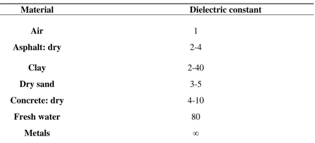
Table 1.1. shows Dielectric constants for some materials.

Table 1.1: Dielectric constant for some materials.

Material Dielectric constant

Air 1 Asphalt: dry 2-4 Clay 2-40 Dry sand 3-5 Concrete: dry 4-10 Fresh water 80 Metals ∞ 1.2.2 GPR Depth Determination

The reflected wave has data on: how much was attenuated and how quickly the signal traveled [5].

The depth of a surface is presented by:

D =

D = depth of object (inch).

t = time of travelling wave (nanosecond). 5.9 = Constant.

Er = Relative permittivity of surface material. 1.2.3 How deep can GPR go into ground? It depends on two conditions:

1-The type of rock or soil in the GPR survey area. 2- The frequency that used of the antenna.

• Low frequency system are more penetrating but resolution of data is low. • High frequency systems have finite penetration but supply a high resolution

1.3 Types of Ground Penetrating Radar

Types of GPR: CW and impulse. Generally most of GPR system are regarded on the impulse penetrating radar and are widespread in the commercial market. stepped-frequency radars and Continues-wave have been improved over the past decade, though most have implicated research universities, institutions, and laboratories. Advanced ways and differences like synthetic aperture radar (SAR) and ultra wideband (UWB) [7].

1.3.1 Impulse GPR

When a data is calculated in time domain by a radar this is called impulse radar. The pulses is transmitted by the domain and the receiver receives the reflected wave in time domain . the major of GPR work as impulse radar. The antenna works a main job in the impulse GPR system as in figure1.3.

Figure 1.3: Impulse GPR system block diagram [7]. 1.3.2 Continuous-Wave GPR

Stepped frequency continuous-wave radar

SFCW GPR system uses separate transmitter and receiver, the signal of the transmitter is received by a radar receiver after reflecting [8].

1.4 GPR Applications Area

GPR application area can be classified in two main application group.in military field, GPR is used for underground warehouses, un exploded bombs, sector room sand also bomb shelter. Besides, in civilian life, it is used for finding buried pipes, undetected blanks and the people who are left under collapsed buildings [9].

In the Science of Earth GPR is worked to detect, soils, bedrocks, water, and ice. [10].

1.5 Three _ Dimensional Imaging

Registration a full-resolution 3D dataset demands a very intensive, whereas in this technique the radar system work to plot the image in 3D and displaying all the information about image and the layer of ground [11]

The example shown below describe the 3D imaging GPR principle.

Figure 1.4: A: Chair display of the Miami Oolite 3D GPR survey [12].

The most important part of GPR system is antenna, improvements in antenna designing way will provide better results in GPR application. SO, in the next chapter fundamental parameters of antenna will be explained.

2. ANTENNA

2.1 Definition

The Antenna is a device used to convert radio frequency into current or vice versa . two types of antenna used in communication systems transmission and receiving antenna . Antenna works a major part in all radio systems and communications [13].

2.2 Radiation Pattern

An antenna pattern or antenna radiation pattern defined as the variation of the power transmitted by an antenna as a function of the direction far away from the antenna. This power deference as a function of the arrival angle is observed in the antenna's far field . Radiation properties include radiation intensity, power flux density, field strength , directivity , polarization or phase [14].

The far field is the area far from the antenna. In this area, the antenna pattern does not change form with distance.[14].

2.2.1 Antenna pattern in 3D

The antenna pattern is a 3D figure and showed in spherical coordinates (r, θ, Φ) regarding its origin at the middle of spherical coordinate system. figure2.1 [15].

Figure 2.1: The 3D Antenna Radiation Pattern [15]. 2.2.2 Antenna Pattern in 2D

The antenna radiation in 2D it represents the vertical and horizontal and it can be represented from 3D radiation pattern. as shown in figure 2.2.

Figure 2.2: The one direction antenna pattern in V and H planes. V plane represents the Vertical pattern, where H plane represents the Horizontal pattern [14]. 2.2.3 Antenna pattern lobes

Different areas of an antenna pattern are classified to as lobes, which may be classified into main or major , back , and side lobes [16].

.

(a) (b)

Figure 2.3: (a) antenna pattern of radiation main lobe .(b) power pattern and radiation[14].

2.3 Intensity of Radiation

Radiation Intensity in a provided guidance is characterized as "the power emanated from an antenna for every unit angle." The intensity of radiation is a far-field parameter, and it very well may be acquired by essentially duplicate the radiation density by the square of the separation . In numerical structure can be gotten as:

U=

(2.1) Where

U= intensity of the radiation (W/unit solid angle) = density of radiation (W/

2.4 Beamwidth

The beamwidth of a radio wire design is characterized as the partition between two indistinguishable focuses on inverse sides of the example most extreme. In antenna pattern, there are difference beamwidths. A most exceptionally utilized beamwidths is the half power beamwidth (HPBW)[17].Another critical beamwidth is the angle division between the main nulls of the radiation design , and it is called to the first null beamwidth (FNBW).

Anyway , by and by , the term beamwidth , with no other recognizable proof , for the most part alludes to the HPBW [17].

Figure 2.4: the two dimensional power pattern [17]. 2.5 Directivity

Isotropic antennas are theoretical point sources that spread electromagnetic energy similarly every which way. The total power radiated is determined by integrating the power flux

density on the surface of a sphere of radius r that surrounds the antenna ( surface area = ) [14].

Antenna directivity is described as "the rate of the radiation power in a provided direction from the antenna to the intensity of the radiation found the middle value of over all bearings. [18].

Maximum directivity can be expressed as

D = directivity (directionless)

Do= highest directivity (directionless)

U= intensity of the radiation ( W/unit sold angle )

= highest intensity of radiation ( W/unit sold angle)

Uo = intensity of the radiation of isotropic source ( W/unit solid angle) = total power radiated (W)

And the maximum directivity written as

Do = (2.4) is the beam solid angle

Figure 2.5: Antenna beam Ω . (a) radiation intensity U from a real antenna . (b) intensity of the radiation with all radiation from the real antenna focused into a cone of solid angle Ω with constant intensity of the radiation equal to the maximum of the

real pattern [14].

The term for changing over the amounts of directivity and most astounding directivity to decibels (dB)are :

D(dB) = 10log10 D _(2.5)

Do(dB) = 10log10 Do (2.6)

2.6 Gain

Gain is One of the useful way to calculate the execution of an antenna.

The intensity of the radiation relating to the isotopically transmitted power is equivalent to the power contribution by the radio wire partitioned by 4π."[13], [14].

Gain = 4π =

(2.7)

Gain =4π = (2.8)

The total power radiated ( ) is concerning to the total power input ( ) by

( ) by

(2.9)

Whereas is the radiation efficiency of antenna (dimensionless) Radiation efficiency can be bounded as

0 ≤ ≥ 1

Then, the antenna gain is equal to its directional directivity multiplied by radiation

efficiency [19] .

G =

Units gain in decibels

G(dB) = 10log10

2.7 Efficiency Of Antenna

The all efficiency of antenna is utilized to take losses at the input and inside the construction of the antenna. As in figure 2.6.

Anyway, the all efficiency can be expressed as

(2.13)

= efficiency of reflection (mismatch) =(1 − ) (dimensionless)

= efficiency of conduction (dimensionless)

= efficiency of dielectric (dimensionless)

Γ = reflection coefficient voltage at the input terminals of the antenna Γ =( − )/( + ) (2.14) Where

VSWR = voltage standing wave ratio = (1 +|Γ|) / (1 −|Γ|)

1- ) (2.15)

Figure2.6: Reference terminal and reference of antenna [14]. Polarization

Antenna Polarization in a genuine way is characterized as "the polarization of Antenna transmitted wave. Note: When the bearing isn't expressed, the polarization is toward greatest gain.”[20].

Polarization might be linear , circular , or elliptical as in Figure2.7.

Figure 2.7: Linear , Circular and Elliptical Polarization[14]

Linear Polarization

Circular Polarization A period consonant wave is circularly polarized at a predetermined spot in space if the magnetic (or electric) field as a component of time .

In the event that the revolution is counterclockwise, the wave is left-hand (or counterclockwise) circularly polarized; if the wave is clockwise, the wave is Right-hand (or clockwise) circularly polarized.

Axial Ratio

It is clear that the pivotal proportion example can be depicted by external and internal envelopes. At any edge, the proportion of the inward and external envelope reactions speak to the pivotal proportion. In the event that the example is perused in decibels, the pivotal proportion is the contrast between the external and inward envelopes (dB); zero dB distinction speaks to roundabout polarization (hub proportion of solidarity).

So thep olarization design is appeared in Figure 2.8[21]

Figure2.8: Radiation Pattern of a polarized circular test antenna given with a rotating, polarized linearly, antenna source. [22].

Elliptical Polarization A period symphonious wave is circularly enraptured if the tip of the field vector (magnetic or electric) follows a elliptical locus in space. [23].

2.8 Input Impedance

Input impedance is characterized as "the impedance depicted by an antenna at its terminals or the proportion of the reasonable segments of the electric to magnetic fields at a point or the proportion of the voltage to current at a couple of terminals."

In Figure2.9 these end points are designated as a – b . The proportion of the voltage to current at these end points [24].

ZA = RA + jXA _(2.16)

Where

ZA= impedance

RA= resistance

XA= reactance

Generally, the resistance is,

RA = Rr+ RL _(2.17)

Where

Rr= antenna radiation resistance

RL=antenna loss resistance

2.9 Return Loss And S11_Parameter

Return loss is a proportion of the proficiency of conveyed power from a transmission line to a load, an antenna return loss is characterized as [25].

(2.20) in term of a transmission line or waveguide the relationship between return loss and reflection coefficient can be expressed as [26].

10 2 10

1

10 log

20 log

RL

dB

dB

=

Γ

= −

Γ

10 log

P

RL

dB

P





=

_

_

_

_





Figure 2.9: Equivalent circuits of transmitting antenna [24]

Rr+RL = Rg _(2.18)

In terms of (VSWR), this is

(2.22)

Low qualities for VSWR speak to a decent antenna coordinate. [26].

S11 is a known starting at how much power is reflected back to the antenna port

since mismatch from the transmission line. S11 values are calculated in dB and

are negative, ex: - 8 dB. S11 is additionally once in a while alluded to as return

loss, which is just S11 however made positive rather (Return Loss = - S11). So if

the reception apparatus Return Loss is 10 dB, S11 is - 10 dB.

In the next chapter, types of antenna will be discussed, which types of antenna is UWB antenna? and which one is appropriate to build GPR system?

These questions will be answered in the next part.

10

1

20 log

1

VSWR

RL

dB

VSWR

+

=

−

3. ANTENNA TYPES

3.1 Wire Antenna

Wire Antennas are the ancient and still the predominant of the antenna form. Wire antennas can be made from either tubular or solid conductors. They are relatively simple concept, easy to fabricate and cheap [13].

3.1.1 Dipole and Monopole Antenna

Dipole, loop, and monopole antennas are the most widely antennas utilized for communication systems, measurements, and broadcasting of magnetic and electric fields [14].

A dipole antenna is generally a metal wire. Generally, a dipole antenna contains two radiating arms symmetrically. A monopole antenna is a singular radiating arm whatever, monopoles are most usually utilized above a full or partial ground plane as in Figure3.1 [15].

Figure 3.1: Dipole and monopole antenna (a) Dipole (b)monopole .[14].

sin , 0 2 2 ( ) sin , 0 2 2 L L Io k z Z I z L L Io k z Z    ₋  _{≤ ≤}    _ _      =       _{+ − ≤ ≤}       _{  }   

It is helpful to visualize the distribution current on the antenna . figure 3.2. Shows the current on the dipole for different lengths.

Figure 3.2. current distribution for various different-fed dipoles [13].

A chart of the variation of the feed-point reactance and resistance of a monopole antenna above ground is given in Figure3.3 as a function of length h/ λ, where λ is the free space wavelength at the radiation frequency [26].

Figure 3.3: Feed point variations R a and reactance X [14]. 3.1.2 Infinitesimal dipole

An infinitesimal Dipole or this is called a Hertzian dipole as in figure 3.4. The magnetic-and electric-field components of the Hertzian dipole are [27].

Figure 3.4: Infinitesimal dipole [13]. 0 ^ 2 1 1 sin 4 jk r jko H IL e r r θ π −   = _ + _ φ   0 ^ 2 3 1 cos 2 jk r o j IL jko E e r ko θ r r π − η   = _ + _   (3.2) 0 2 _^ 2 3 1 sin 2 jk r o o o j IL k jk e ko θ r r r θ π −   η − _− + + _  

The total power radiated is =40π

İ

(L/ λ )

3.1.3 Folded dipole antennas

Figure 3.6: Folded dipole antenna [14].

Zt= jZo tanβ (3.3) The input impedance Zt for this mode is given by the equation for a transmission line with a short circuit load .

3.1.4 Log-periodic antenna

log-periodic antennas are generally utilized as transmitter and receiver antennas. The shape of a log periodic array is in Figure 3.

(3.4)

where τ = / [15].

(3.5)

Figure 3.7: Log periodic dipole array(a)log periodic and (b) its equivalent [15]. 22

3.1.5 Broad band dipole arrays

A broadband dipole curtain like in Figure3.8 is usually utilized for high power .

Figure 3.8: A broadband dipole curtain [14]. 3.1.6 Yagi uda dipole array

Yagi Uda arrays are usually utilized as general aim antennas, in special, as TV antennas. They are cheap, have credible bandwidth. They have single direction beamwidth [14]. As in Figure 3.9.

Figure 3.9: Yagi Uda array [15]. 3.2 Microstrip Antenna

Printed antennas are constructed using printed circuit fabrication techniques like a portion of the metal layer is responsible for radiate power . [13, 14] [15]. In high execution spacecraft ,aircraft, missile, and satellite applications, where weight, size, performance, cost, ease of installation, and aerodynamic profile are constraints, low-profile antennas may be required. Recently there are many other commercial and government applications, like wireless and mobile radio

communications, that have same specifications. To achieve these demands, microstrip antennas can be utilized. These antennas are simple and cheap .[15]. 3.2.1 Microstrip patch antenna

Microstrip device in its simplest form is a layered structure with two conductors parallel inserted by a small dielectric substrate and the lower conductor playing as a ground plane. If the upper metallization is a long narrow strip, a microstrip transmission line is formed as shown in Figure3.11. Conventional patch designs yield bandwidths as low as a few percent. The resonant nature of microstrip antennas also means that at frequencies below UHF they become excessively large [13].

An approximate value for the length of a resonant half-wavelength patch is [13].

L = 0.49

= 0.49

Half wave patch (3.8)

is

.

Input impedances at the edge of a rectangular resonant patch.[13].

(3.9)

Figure 3.10: The rectangular patch microstrip antenna [13].

The microstrip antenna width w controls the input impedance Microstrip field are plotted in figure3.12 for L=W=0.5 λ

Figure 3.11: the fields of the microstrip antenna at W=L=0.5 λ[13]. Travelling Wave Antenna

3.2.2 Helical antenna

Simple, practical, and basic representation of an electromagnetic radiator is a helix, as shown in Figure 3. 13. In most condition the helix is utilized with a ground plane.as shown in figure 3.12 [20].

The geometric representation of a helix depends generally of N turns, spacing S and diameter D between each turn. The total length of the antenna is L = NS whereas the total length of the wire is = NLo = N where Lo =

is the wire length between each turn and the circumference is C =

πD of the helix. [1].

Figure 3.12: Helical antenna with ground plane [20].

Figure 3.13: Commercial helix [13]. Figure 3.14 Design of helix [13].

Figure 3.14: Design of helix[13]. 3.2.3 SpiralAntennas

Spiral antennas and their differences are generally constructed to be either nearly or exactly self complementary. This achieve wide bandwidth.

• Equiangular Spiral Antenna

The equiangular spiral curve shown in Figure. 24 is given by the generating equation.

r = (3.11)

where ro is the radius for = 0 and a is a controlling constant the spiral flare

rate . The spiral of Figure 3.16 is right handed. If the values of

is negative

the left hand spirals can be generated, or by simply turning over the spiral of Fig3.17. The curve of the equiangular spiral is used to create the antenna of Figure3. 25 [28]. Which indicate Planar equiangular spiral antenna.

Figure3.15: curve of the Equiangular spiral with r= and

Figure 3.16: Planar equiangular spiral antenna [28]. • Archimedean Spiral Antenna

Different shape of the planar spiral is the Archimedean spiral antenna in Figure3.18. This antenna, as are many spiral antennas, is readily fabricated . The equation of the two spirals in Figure 3.26 are

r = and (3.12)

Figure 3.17: Archimedean spiral antenna [28].

3.3 Aperture Antenna 3.3.1 Vivaldi antenna

Vivaldi Antenna is a broadband antenna, which can be fabricate from a solid piece of metal sheet, board of a printed circuit , or from a dielectric substrate on one or both sides as in figure 3.19 [27].

The feeding line excites an open space via a coaxial cable or microstrip line, and may be terminated with a shaped sector area or a coaxial connection direct. Vivaldi antennas can be fabricate for linear wave polarized or using two devices putted in orthogonal direction for transmitter , receiver both polarization orientations[27].

Vivaldi antennas are work for any frequency.

Advantages of Vivaldi antennas are their wide broadband Antenna , their easy fabricating process , low cost , end-fire radiation.[28].

Figure 3.18: Vivaldi Antenna [28]. 3.3.2 Horn antenna

Types Of Antenna Horn 1. Pyramidal horn

An antenna Horn with the horn in the form of a four sided pyramid, with a rectangle cross section [29].

2. E-plane horn

A radiation in the direction of the E-field in the waveguide.

3. H-plane horn

4. Conical horn

A horn in the shape of a cone , with a circle cross section. As in figure 3.20.

Figure 3.19: Typical electromagnetic horn antenna configurations [13].

In the next chapter, candidate Antenna and methodology of designing with results will be introduced.

4. METHODOLOGY AND RESULTS DISCUSSION

4.1 Antipodal Vivaldi Antenna (AVA).

Designing (AVA) starts from choosing the dimensions and substrate material that will assist to give a good reading in radiation pattern and return loss , after that we will move to any other additional techniques like dielectric lens , elliptical curve edges , that make any enhancement for required readings .

In this design we will discuss all factors that used for design, and how each factor made an improvement in the results. The antenna fed by 50 ohm coplanar waveguide and simulated by CST studio suit program 2018.

Figure 4.1(a) represents the structure of the proposed AVA with dimensions of 50 × 70mm2 on a substrate of Taconic with dielectric constant of 3.55, tangent loss of 0. 0025 and 0.76 mm height. The antenna consists from one plate and two slots at front and back sides the thickness of slots are 0.035 mm.

But this design suffers from low and inconsistent gain and directivity.

For this, a dielectric lens is added as shown in figure 4.1. (b). The lens tends to limit their wide spread utilization. They are costlier due to complex fabrication process

For getting a good radiation pattern at low frequencies too and to make improvement in S11 parameter readings an elliptical curvature edge is inserted to

Figure 4.1: AVAs. (a) Typical AVA . (b) AVA with lens .(c) Proposed AVA. According to figure 4.2.(a) the highest reading of proposed antenna was at 15 GHz (10.2dBi), whereas at Typical AVA and AVA with lens the highest gain was less than this result .Moreover at low frequencies at 3 GHz the reading when antenna designed with elliptical curvature edge the reading raised to 7.4 dBi , although the first result was at 5.7 dBi.

(a) (b)

Figure 4.2: Simulated gain. (a) Typical AVA ,AVA with lens and Proposed Antenna.(b) Proposed AVA with different T Distance.

On another hand , the gain is varied depending on shape of the curvature and length of the taper [30],according to the form of curvature the distance between two curves at slot T have revers relation with gain at high frequencies as shown in figure 4.2.(b).

When T=5.5 mm at 15 GHz the gain is 12.2 dBi , and T= 8 mm at same frequency the gain is 11.8 dBi, but the proposed antenna with T=15 mm has the advantage with highest gain at low frequency 3 GHz with gain is 7.4 dBi

.whereas at the same frequency the readings were 6.1 and 6 dBi at T=5.5 and T=8mm respectively.

Figure 4.3: (a) Proposed AVA ,(b) Proposed AVA two slots

Figure 4.3. represent the proposed antenna table 4.1 shows the dimensions of the Antenna , with AVA the dielectric lens is utilized to enhance various specifications of the Vivaldi antennas, is utilized to increase gain of the antenna as represented in figure4.3.(a) , in order to the lens shape and its dielectric constant are most important parameter in its design [13-14]. Besides shape, dielectric constant of the lens works an important job in the antenna’s specifications. High dielectric constant supplies higher gain and more beam directed.

To improve the S11 reading the elliptical curved edge is inserted to design with

this dimensions , these edges play to make S11 < -10 dB at low frequencies in

this design by this dimensions.

Figure 4.4(a). represent the S11 readings of the antennas and figure 4.4(b).

Represent S11 readings of Proposed antenna at different T distances .

Table 4.1: Proposed AVA Dimensions.

Parameter Value(mm) parameter Value(mm)

L 70 D1 14 L1 60 D2 17 L2 8.85 W1 2 L3 18.35 T 15 SL 15 R 10 W 50

Figure 4.4: S11 simulations ,(a) Typical AVA, AVA with lens , Proposed AVA , (b) Proposed AVA at different T Distance.

According to figure 4.4(a) typical AVA and AVA with lens have the S11 reading

to whole frequency range and the S11 < -10 dB start from 4.9 GHz , it means at

low frequency these designs don’t work in good way, by this information the dielectric lens doesn’t has a role to make improvement in S11 reading at low

frequency , whereas when Proposed AVA designed with elliptical curvature edges , these edges work to improve S11 reading at low frequency and enhances

the reading in high frequency , as shown in figure 4.4 (a) proposed AVA has S11

reading < -10 dB at whole frequency band .

According to this readings the elliptical curvature edges are most important parameter for design this AVA with good S11 readings at low frequencies.

In figure 4.4.(b) S11 reading for proposed Antenna at T=15 mm is better than at

T=5.5 and T=8 mm , as showed in the figure at T=5.5 and 8 mm the S11 reading

is same at whole frequency band , but when T= 15 mm the reading is improved at low frequency at 3 GHz to be less than -10 dB.

Proposed AVA with this design with dimensions has the best radiation pattern and S11 parameter reading.

All factors work together to apply this requirements, it depends on each others The radiation pattern in 3D at low and high frequency are presented in figure 4.5 . The antenna produce symmetrical antenna pattern in H-plane and E-plane[11] .

(a) (b) (c) Figure 4.5: simulation radiation pattern of the antenna . (a) 3GHz. (b) 8.9 GHz.

(c)15 GHz.

Table 4.2. recognize the antenna compression with other antennas literature according to The design and lens and the gain improvement with operational frequency.

Table 4.2: Comparison of Antenna Characteristic and literature.

REF. Dimensions (mm3) Frequency (GHz) Relative Permittivity and material Freq(GHz) Gain(dB) [30] 178×140×251 0.83-12.8 2.2 AN-79 0.83 0 12 10 [31] 96×50×3.15 3-18 2.55 ArlonAD255 3 5 18 14 [32] 130×76×1 3.1-14 4.2 FR4 3.1 5.8 10 7.26 [33] 40×90×0.508 3.8-40 3.3 RO4003C 3.4 8 19.5 12.8 This work 70×50×0.76 2.8-15 3.55 Taconic 3 5.2 15 9.9

(a)

(b)

(c)

Figure 4.6: Antenna pattern of the antenna. (a)3 GHz . (b) 8.9 GHz . (c) 15 GHz. Figure 4.6. represent the radiation pattern of the antenna H-Field and E-field , it appears that at high frequency the radiation pattern is better than at low

frequency, for instance at 15 GHz E-Field is 15 dBV/m in direction of 90o and with angular width 60o ,whereas the angular width is the distance between the two half power beam width (HPBM) , for H-Field is -36.6 dBA/m at the same frequency in the direction in the same of E-Field.

4.2 Double Slot Antipodal Vivaldi Antenna (DSAVA).

DSAVA is a technique used to enhance directivity or radiation pattern, in this design the antenna is fed by 50 ohm coplanar wave guide and designed by FR4 substrate material of dielectric constant 4.3 . The first step is to choose the dimension of the antenna and the thickness of the substrate material after that we added some additional technique that assist to enhance the radiation characteristics like dielectric lens, the antenna is simulated by CST Suit Studio program 2018 , and fed by 50 ohm coplanar wave guide.

Figure 4.7 (a) represents the geometry of the proposed AVA with dimensions of 50 × 70 mm2 on a substrate of FR4 of dielectric constant of 4.3, tangent loss of 0. 025 and 1 mm height. The antenna consists from one plate and two slots at front and back sides the thickness of slots are 0.035 mm.

Actually , the elliptical shape is added to enhance some parameters , but in this design unfortunately, this technique did not add any improvement to results as in figure 4.7 .(b). To enhance the directivity and radiation pattern a dielectric lens is added to design as shown in figure 4.7 .(c), whereas a dielectric lens play good role to limit their wide spread utilization. They are costlier due to complex fabrication process .

Figure 4.7: configuration of DSAVA . (a) Typical DSAVA. (b) DSAVA with elliptical shape . (c) Proposed DSAVA.

Figure 4.8 represents the S11 parameter reading of these designs , according to

the figure 8 the DSAVA without lens has a good reading at low frequencies whereas the reading < -10 dB starts at 3.5 GHz and still until whole frequency band , but when dielectric lens is added figure 1 (c) the reading has a little enhancement at low frequency where the reading still starts at 3.5 GHz and stay until whole frequency band.

Figure 4.8: S11 simulations . Typical DSAVA , elliptical shape, cylinder shape and

Proposed DSAVA.

When elliptical shape is added to design figure 4.7 (b), the S11 reading was not

affected at low frequency it means this technic dose not has enhancement at S11

reading in DSAVA design.

In the same way the cylinder shape is added as another technic , but this method gave a negative results at low frequencies where the reading goes above -10 dB from 3.5 to 6 GHz as in figure 4.7.

Figure 4.9: (a) Proposed DSAVA , (b) Proposed DSAVA two slots.

Figure 4.9. represents the Proposed DSAVA the dimensions of the antenna represented in Table 4.3, the dielectric lens is used to enhance various characteristics of the Vivaldi antennas, is used to enhance gain of the antenna as represented in figure 4.11, in order to the lens shape and its dielectric constant are most important parameter in its design [31-33].

-60 -55 -50 -45 -40 -35 -30 -25 -20 -15 -10 -5 0 2 3 4 5 6 7 8 9 10 11 12 13 14 15 16 dB Frequency/ GHz S - Parameter Typical DSAVA elliptical shape cylinder shape Proposed DSAVA 38

With shape, dielectric constant of the lens works an important job in the antenna’s specifications. High dielectric constant supplies high gain and more beam directed.

Figure 4.10: Kimulated gain. Typical DSAVA , elliptical shape , cylinder shape , Proposed DSAVA .

Table 4.3: Proposed DSAVA Dimensions.

Parameters Value (mm) Parameters Value(mm)

L 70 W 50

L1 20 W1 2

X1 50 W2 25

X2 20 W3 1

SL 9 R 18

Proposed DSAVA with this dimensions and this design has the best radiation pattern and S11 parameter reading at low and high frequency , all parameter

work together to achieve this results.

The radiation pattern in 3D at low and high frequency are presented in figure 4.11 . The antenna produce symmetrical antenna pattern in H-plane and E-plane[31] . 3 4 5 6 7 8 9 10 11 12 13 14 15 2 3 4 5 6 7 8 9 10 11 12 13 14 15 16 dB i Frequency / GHz Gain Typical DSAVA elliptical shape cylinder shape Proposed DSAVA

(a) (b) (c)

Figure 4.11: Simulation radiation pattern of the Proposed DSAVA (a) 4 GHz , (b) 9.05 GHz , (c) 15 GHz.

Table 4.4 recognize the antenna compression with other antennas literature according to the design and lens and the gain improvement with operational frequency.

Table 4.4: Comparison of Antenna Characteristic and literature REF. Dimensions (mm3) Frequency (GHz) Relative Permittivity and material Freq(GHz) Gain(dB) [30] 178×140×251 0.83-12.8 2.2 AN-79 0.83 0 12 10 [34] 50×150×1 2-18 4.3 FR4 2 0 18 5.3 [31] 96×50×3.15 3-18 2.55 ArlonAD255 3 5 18 14 [32] 130×76×1 3.1-14 4.2 FR4 3.1 5.8 10 7.26 [33] 40×90×0.508 3.8-40 3.3 RO4003C 3.4 8 19.5 12.8 This work 70×50×1 3-15 4.3 FR4 4 5.57 15 10.3 40

(a)

(b)

(c)

E-Field pattern H-Field pattern Figure 4.12: antenna pattern. (a) 3.55 GHz . (b) 9.05 GHz . (c) 15 GHz.

Figure 4.12. represents the radiation pattern H-field and E-Field of the antenna at different frequencies , we notice that at high frequencies the radiation pattern is better than at low frequencies , in comparison of the radiation pattern in DSAVA is better than in AVA.

4.3 CST Studio Suite

The CST Studio Suite design environment is common across all the modules. Comprising a 3D interactive model tool and a layout tool, the electromagnetic

(EM) design environment combines a pre processor for the solvers, post-processing tools tailored to industry needs, and an intuitive user interface for model construction and solver set-up.

Figure 4.13: CST Studio 3D interactive modeling.

The two antennas are simulated , each one in different dimensions , different substrate material and different shape , the methodology and results are discussed .

5. CONCLUSION

This thesis was about Ground Penetrating Radar (GPR) is a radar which detects objects under the ground . The GPR system usually consists of receiving and transmitting device , transmitter connected with a source, and receiver connected with signal processing. The antennas type and antenna’s efficiency is also an important part of the system. So, the antenna plays an important role in GPR .

GPR used in UWB application, therefor GPR required an UWB Antenna to design its system so, after a comparative study between all types of antenna as in chapter 3 and the specification of each type, one of the best UWB antennas has been used to build GPR system is Vivaldi Antenna , it refer for its end-fire radiation , moderate gain, small dimensions, and easy fabrication.

Two types of Vivaldi Antenna are designed in this thesis, one is Antipodal Vivaldi Antenna (AVA) and other one is Double Slot Antipodal Vivaldi Antenna (DSAVA) , each one of these antennas has some properties different than other one , starting from antenna shape until to the results as in chapter 4. In this work , AVA with exponentially dielectric lens and elliptical curvature edge for GPR application has been introduce. The proposed geometry presents an introduce in radiation pattern of an antenna . working a dielectric lens enhance the radiation characteristic than when it hasn’t introduced . Moreover, elliptical curvature edges improved the return loss (S11) characteristics at low

frequency , the substrate material that used is Taconic and the highest radiation pattern is 10.3 dBi at 15 GHz , although it has a good reading of radiation pattern at low frequency 7.4 dBi at 3 GHz. So, this proposed is a good candidate for UWB application and GPR.

In another hand , DSAVA is proposed with dielectric lens , DSAVA has an advantage because it produced to enhance directivity and radiation pattern , it is appear in the radiation characteristic is better than in AVA , in additional of

dielectric lens tend to enhance radiation characteristic especially at high frequency.

The substrate material is FR4 with dielectric constant 4.3 , and the highest radiation pattern is 13.9 dBi at 15 GHz , in another side at 4 GHz is 6.7 dBi . The presented structure proves stable radiation characteristics with the all range of frequencies, which makes it a good candidate for GPR and UWB application.

REFFERENCES

[1] A. D. Zhang College of Resource Environment and Tourism, Capital Normal University, No.105, North West 3rd Ring Road Haidian District, 100048, Beijing,china.

[2] B. J.C. Li

College of Resource Environment and Tourism, Capital Normal University, No.105, North West 3rd Ring Road Haidian District, 100048, Beijing, China.

[3] http://www.nesubsurface.com/index.php/equipment/gpr-equipment

[4] Conyers, Lawrence B. and Dean Goodman (1997) Ground-Penetrating

Radar: An Introduction for Archaeologists. Altimira Press, Walnut

Creek.

[5] Daniels DJ (ed.) (2004).Ground Penetrating Radar (2nd ed.). Knoval (İnstitution of Engineering and Technology ).pp.1-4. İSBN 978-0-86341-360-5

[6] Derald G. Smith, Harry M. Jol, Ground penetrating radar: antenna frequencies and maximum probable depths of penetration in Quaternary sediments.

[7] HARRY M . JOL, Ground Panetrating Radar Theory And Applications, first edition , 2009.

[8] V.G. Sugak, "Reconstruction of Electrical Constants of Soil and Depth of Subsurface Objects Using Data of Subsurface Sounding", Telecommunication and Radio Engineering, vol. 59, no. 1 & 2, pp. 54-63, 2003.

[9] Saeid KARAMZADEH, Ahmet Said HEPBİÇER, FatihDEMİRBAŞ,Oğuz Furkan KILIÇ ‘Double Band Fractal Bow Tie Antenna Design for GPR Application’ 2017.

[10] Wilson, M. G. C.; Henry, G.; Marshall, T. R. (2006). "A review of the alluvial diamond industry and the gravels of the North West Province, South Africa" (PDF). South African Journal of Geology. Geological Society of South Africa. 109 (3): 301– 314. doi:10.2113/gssajg.109.3.301. Retrieved 9 December 2012.

[11] M.Grasmueck, R.Weger, H.Horstmeyer “ Full-resolution 3D GPR imaging for geoscience and archeology’’.

[12] Hoffmeister, J.E., Stockman, K.W., and Multer, H.G., 1967, Miami

Limestone of Florida and its Recent Bahamian counterpart: Geological Society of America Bulletin, vol.78, no.2, p.175-189.

[13]Warren L. Stutzman, Gary A. Thiele ‘’ Antenna Theory And Design 3rd Edition ‘’2012.

[14] Constantine A. Balanis ‘’ Modern Antenna Handbook,John Willy 2008 ‘’ [15] W.R.Scott JR. A general program for plotting three-dimensional antenna

[16] C.A. Balanis , Antenna Theory : Analysis and Design (3rd eds) 2005. [17] NEIL K. JABLON, Effect of Element Errors on Half-Power Beamwidth of

the Capon Adaptive Beamformer, İEEE , july 1987.

[18] J.D. Kraus and R.J. Marhefka, Antenna, McGraw-Hill, New York 2002 [19] J.D.Kraus, Radio Astronomy, McGraw-Hill, New York 1966

[20]. C. A. Balanis, Advanced Engineering Electromagnetics , John Wiley & Sons, Hoboken, NJ, 1989.

[21] G. A. Deschamps, Part II—Geometrical representation of the polarization of a plane electromagnetic wave, Proc. IRE , Vol. 39, pp. 540–544, May 1951.

[22]. G. Sinclair, The transmission and reflection of elliptically polarized waves, Proc. IRE , Vol. 38, pp. 148–151, February 1950.

[23] C. A. Balanis, Antenna theory: a review, Proc. IEEE , Vol. 80, No. 1, pp. 7–23, January 1992.

[24] E. S. Gillespie, “Measurement of Antenna Radiation Characteristics on Far-Field Ranges,” Chapter 32 in Antenna Handbook (Y. T. Lo and S. W. Lee, eds.), pp. 32-1–32-91, Van Nostrand Reinhold Co., Inc., New York, 1988.

[25] D. M Pozar, Microwave Engineering, New York:AddisonWesley, 1990. p. 633f.

[26] E. C. Jordan and K. G. Balmain, Electromagnetic Waves and Radiating Systems , 2nd ed., Prentice Hall, Englewood Cliffs, NJ, 1968.

[27] R. C. Johnson (Ed.), Antenna Engineering Handbook , 3rd ed., McGraw-Hill, New York, 1993.

[28] G. A. Thiele, Analysis of Yagi–Uda type antennas, IEEE Trans. Antennas Propag. , Vol. 14, No. 5, pp. 648–649, September 1966.

[29] Montoya, T.P. and Smith, G.S., 1996, A study of pulse radiation from several broad-band loaded monopoles: IEEE Trans. Antennas Propagat., v. AP-44, no. 8, p. 1172–1182.

[30] Jinjin Shao, Guangyou Fang, Jingjing Fan, YiCai Ji, and Hejun Yin” TEM Horn Antenna Loaded With Absorbing Material for GPR Applications,” IEEE ANTENNAS AND WIRELESS PROPAGATION LETTERS, VOL. 13, 2014.

[31] Ziani Tahar, Xavier D´erobert, and Malek Benslama, “An Ultra-Wideband Modified Vivaldi Antenna Applied to Ground and Through the Wall Imaging,” Progress In Electromagnetics Research C, Vol. 86, 111– 122, 2018.

[32] Majid Amiri, Farzad Tofigh, Student Member, IEEE, Ali Ghafoorzadeh-Yazdi, Member, IEEE, and Mehran Abolhasan, Senior Member, IEEE,” Exponential Antipodal Vivaldi Antenna With Exponential Dielectric Lens,” IEEE ANTENNAS AND WIRELESS PROPAGATION LETTERS, VOL. 16, 2017.

[33] M. Moosazadeh and S. Kharkovsky, “A compact high-gain and front-toback ratio elliptically tapered antipodal Vivaldi antenna with trapezoidshaped dielectric lens,” IEEE Antennas Wireless Propag. Lett., vol. 15, pp. 552–555, 2016.

[34] Youngmin So1, Woojoong Kim1, Jaesik Kim1, Young Joong Yoon1, and Jinsung Park2 “

Double-slot Antipodal Vivaldi Antenna for Improved Directivity and Radiation Patterns “, 1Department of Electrical and Electronic Engineering,

Yonsei University, Seoul, Republic of Korea 2Agency for Defense Development.

RESUME

Name Surname: Bader Awad

Place and Date of Birth : 05/07/1990 , Palestine (Filistin) Education:

• Bachelor : 2014 , Palestine Polytechnic

University in Palestine, Institute of Electrical and Electronics Engineering , Electronics and Communications Engineering.

• Master : 2019, Istanbul Aydin University , Turkey, Department of Electrical and Electronics Engineering , Electrical and Electronics