Research Article
An Improved Demand Forecasting Model Using
Deep Learning Approach and Proposed Decision
Integration Strategy for Supply Chain
Zeynep Hilal Kilimci ,
1A. Okay Akyuz ,
1,2Mitat Uysal,
1Selim Akyokus ,
3M. Ozan Uysal,
1Berna Atak Bulbul ,
2and Mehmet Ali Ekmis
21Department of Computer Engineering, Dogus University, Istanbul, Turkey 2OBASE Research & Development Center, Istanbul, Turkey
3Department of Computer Engineering, Istanbul Medipol University, Istanbul, Turkey
Correspondence should be addressed to Berna Atak Bulbul; [email protected] Received 1 February 2019; Accepted 5 March 2019; Published 26 March 2019 Guest Editor: Thiago C. Silva
Copyright © 2019 Zeynep Hilal Kilimci et al. This is an open access article distributed under the Creative Commons Attribution License, which permits unrestricted use, distribution, and reproduction in any medium, provided the original work is properly cited.
Demand forecasting is one of the main issues of supply chains. It aimed to optimize stocks, reduce costs, and increase sales, profit, and customer loyalty. For this purpose, historical data can be analyzed to improve demand forecasting by using various methods like machine learning techniques, time series analysis, and deep learning models. In this work, an intelligent demand forecasting system is developed. This improved model is based on the analysis and interpretation of the historical data by using different forecasting methods which include time series analysis techniques, support vector regression algorithm, and deep learning models. To the best of our knowledge, this is the first study to blend the deep learning methodology, support vector regression algorithm, and different time series analysis models by a novel decision integration strategy for demand forecasting approach. The other novelty of this work is the adaptation of boosting ensemble strategy to demand forecasting system by implementing a novel decision integration model. The developed system is applied and tested on real life data obtained from SOK Market in Turkey which operates as a fast-growing company with 6700 stores, 1500 products, and 23 distribution centers. A wide range of comparative and extensive experiments demonstrate that the proposed demand forecasting system exhibits noteworthy results compared to the state-of-art studies. Unlike the state-of-art studies, inclusion of support vector regression, deep learning model, and a novel integration strategy to the proposed forecasting system ensures significant accuracy improvement.
1. Introduction
Since competition is increasing day by day among retailers at the market, companies are focusing more predictive analytics techniques in order to decrease their costs and increase their productivity and profit. Excessive stocks (overstock) and out-of-stock (stockouts) are very serious problems for retailers. Excessive stock levels can cause revenue loss because of company capital bound to stock surplus. Excess inventory can also lead to increased storage, labor, and insurance costs, and quality reduction and degradation depending on the type of the product. Out-of-stock products can result in
lost for sales and reduced customer satisfaction and store loyalty. If customers cannot find products at the shelves that they are looking for, they might shift to another competitor or buy substitute items. Especially at middle and low level segments, customer’s loyalty is quite difficult for retailers [1]. Sales and customer loss is a critical problem for retailers. Considering competition and financial constraints in retail industry, it is very crucial to have an accurate demand forecasting and inventory control system for management of effective operations. Supply chain operations are cost oriented and retailers need to optimize their stocks to carry less financial risks. It seems that retail industry will face more
Volume 2019, Article ID 9067367, 15 pages https://doi.org/10.1155/2019/9067367
competition in future. Therefore, the usage of technological tools and predictive methods is becoming more popular and necessary for retailers [2]. Retailers in different sectors are looking for automated demand forecasting and replenish-ment solutions that use big data and predictive analytics technologies [3]. There has been extensive set of methods and research performed in the area of demand forecasting. Traditional forecasting methods are based on time-series forecasting approaches. These forecasting approaches predict future demand based on historical time series data which is a sequence of data points measured at successive intervals in time. These methods use a limited number of historical time-series data related with demand. In the last two decades, data mining and machine learning models have drawn more attention and have been successfully applied to time series forecasting. Machine learning forecasting methods can use a large amount of data and features related with demand and predict future demand and patterns using different learning algorithms. Among many machine learning methods, deep learning (DL) methods have become very popular and have been recently applied to many fields such as image and speech recognition, natural language processing, and machine trans-lation. DL methods have produced better predictions and results, when compared with traditional machine learning algorithms in many researches. Ensemble learning (EL) is also another methodology to boost the system performance. An ensemble system is composed of two parts: ensemble gen-eration and ensemble integration [4]. In ensemble gengen-eration part, a diverse set of base prediction models is generated by using different methods or samples. In integration part, the predictions of all models are combined by using an integration strategy.
In this study, we propose a novel model to improve demand forecasting process which is one of the main issues of supply chains. For this purpose, nine different time series methods, support vector regression algorithm (SVR), and DL approach based demand forecasting model are constructed. To get the final decision of these models for the proposed system, nine different time series methods, SVR algorithm, and DL model are blended by a new integration strategy which is reminiscent of boosting ensemble strategy. The other novelty of this work is the adaptation of boosting strategy to demand forecasting model. In this way, the final decision of the proposed system is based on the best algorithms of the week by gaining more weight. This makes our forecasts more reliable with respect to the trend changes and seasonality behaviors. The proposed system is implemented and tested on SOK Market real-life data. Experiment results indicate that the proposed system presents noticeable accuracy enhance-ments for demand forecasting process when compared to single prediction models. In Table 3, the enhancements obtained by the novel integration method compared to single best predictor model are presented. To the best of our knowl-edge, this is the first study to consolidate the deep learning methodology, different time series analysis models, and a novel integration strategy for demand forecasting process. The rest of this paper is organized as follows: Section 2 gives a summary of related work about demand forecasting, time series methods, DL approach, and ensemble learning
methodologies. Section 3 describes the proposed framework. Sections 4, 5, and 6 present experiment setup, experimental results, and conclusions, respectively.
2. Related Work
This section gives a summary of some of researches about demand forecasting, EL, and DL. There are many appli-cation areas of automatic demand forecasting methodolo-gies at the literature. Energy load demand, transportation, tourism, stock market, and retail forecasting are some of important application areas of automatic demand forecasting. Traditional approaches for demand forecasting use time series methods. Time series methods include Na¨ıve method, average method, exponential smoothing, Holt’s linear trend method, exponential trend method, damped trend methods, Holt-Winters seasonal method, moving averages, ARMA (Autoregressive Moving Average), and ARIMA (Autoregres-sive Integrated Moving Average) models [5]. Exponential smoothing methods can have different forms depending on the usage of trend and seasonal components and additive, multiplicative, and damped calculations. Pegels presented different possible exponential smoothing methods in graphi-cal form [6]. The types of exponential smoothing methods are further extended by Gardder [7] to include additive and mul-tiplicative damped trend methods. ARMA and ARIMA (also called the Box–Jenkins method named after the statisticians George Box and Gwilym Jenkins) are most common methods that are applied to find the best fit of a model to historical values of a time series [8].
Intermittent Demand Forecasting methods try to detect intermittent demand patterns that are characterized with zero or varied demands at different periods. Intermittent demand patterns occur in areas like fashion retail, automotive spare parts, and manufacturing. Modelling of intermittent demand is a challenging task because of different variations. One of the influential methods about intermittent demand forecasting is proposed by Croston [9]. Croston’s method uses a decomposition approach that uses separate exponentially smoothed estimates of the demand size and the interval between demand incidences. Its superior performance over the single exponential smoothing (SES) method has been demonstrated by Willemain [10]. To address some limitations on Croston’s method, some additional studies were per-formed by Syntetos–Boylan [11, 12] and Teunter, Syntetos, and Babai [13]. Some applications use multiple time series that can be organized hierarchically and can be combined using bottom up and top down approaches at different levels in groups based on product types, geography, or other features. A hierarchical forecasting framework is proposed by Hydman et al. [14] that provides better forecasts produced by either a top-down or a bottom-up approach.
On supply chain context, since there are a high number of time series methods, automatic model selection becomes very crucial [15]. Aggregate selection is a single source of forecasts and is chosen for all the time series. Also all combinations of trend and cyclical effects in additive and multiplicative form should be considered. Petropoulos et al. in 2014 analyzed via regression analysis the main determinants of forecasting
accuracy. Li et al. introduced a revised mean absolute scaled error (RMASE) in their study as a new accuracy measure for intermittent demand forecasting which is a relative error measure and scale-independent [16]. In addition to time series methods, artificial intelligence approaches are becoming popular with the growth of big data technologies. An initial attempt was made in the study of Garcia [17].
In recent years, EL is also popular and used by researchers in many research areas. In the study of Song and Dai [18], they proposed a novel double deep Extreme Learning Machine (ELM) ensemble system focusing on the problem of time series forecasting. In the study by Araque et al., DL based sentiment classifier is developed [19]. This classifier serves as a baseline when compared to subsequent results proposing two ensemble techniques, which aggregate baseline classifier with other surface classifiers in sentiment analysis. Tong et al. proposed a new software defect predicting approach including two phases: the deep learning phase and two-stage ensemble (TSE) phase [20]. Qiua presented an ensemble method [21] composed of empirical mode decomposition (EMD) algorithm and DL approach both together in his work. He focused on electric load demand forecasting prob-lem comparing different algorithms with their ensemble strategy. Qi et al. present the combination of Ex-Adaboost learning strategy and the DL research based on support vector machine (SVM) and then propose a new Deep Support Vector Machine (DeepSVM) [22].
In classification problems, the performance of learning algorithms mostly depends on the nature of data repre-sentation [23]. DL was firstly proposed in 2006 by the study of Geoff Hinton who reported a significant invention in the feature extraction [24]. After then, DL researchers generated many new application areas in different fields [25]. Deep Belief Networks (DBN) based on Restricted Boltzmann Machines (RBMs) is another representative algorithm of DL [24] where there are connections between the layers but none of them among units within each layer [24]. At first, a DBN is implemented to train data in an unsupervised learning way. DBN learns the common features of inputs as much as possible it can. Then, DBN can be optimized in a supervised way. With DBN, the corresponding model can be constructed for classification or other pattern recognition tasks. Convolutional Neural Networks (CNN) is another instance of DL [22] and multiple layers neural networks. In CNN, each layer contains several two-dimensional planes, and those are composed of many neurons. The main principal advantage of CNN is that the weight in each convolutional layer is shared among each of them. In other words, the neurons use the same filter in each two-dimensional plane. As a result, feature tunable parameters reduce computation complexity [22, 25]. Auto Encoder (AE) is also being thought to train on deep architectures in an acquisitive layer-wise manner [22]. In neural network (NN) systems, it is supposed that the output itself can be thought as the input data. It is possible to obtain the different data representations for the original data by adjusting the weight of each layer. Input data is composed of encoder and decoder. AE is a NN for reconstructing the input data. Other types of DL methods can be found in [24, 26, 27].
Our work differs from the above mentioned literature studies in that this is the very first attempt of employing dif-ferent time series methods, SVR algorithm, and DL approach for demand forecasting process. Unlike the literature studies, a novel final decision integration strategy is proposed to boost the performance of demand forecasting system. The details of the proposed study can be found in Section 3.
3. Proposed Framework
This section gives a summary of base forecasting techniques such as time series and regression methods, support vector regression model, feature reduction approach, deep learning methodology, and a new final decision integration strategy.
3.1. Time Series and Regression Methods. In our proposed
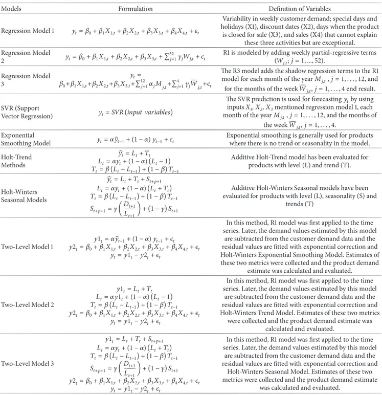
system, nine different time series algorithms including mov-ing average (MA), exponential smoothmov-ing, Holt-Winters, ARIMA [28] methods, and three different Regression Models are employed. In time series forecasting models, the classical approach is to collect historical data, analyze these data underlying feature, and utilize the model to predict the future [28]. Table 1 shows algorithm definitions and parameters which are used in the proposed system. These algorithms are commonly used forecasting algorithms in time series demand forecasting domain.
3.2. Support Vector Regression. Support Vector Machines
(SVM) is a powerful classification technique based on a supervised learning theory developed and presented by Vladimir Vapnik [29]. The background works for SVM depend on early studies of Vapnik’s and Alexei Chervo-nenkis’s on statistical learning theory, about 1960s. Although the training time of even the fastest SVM can be quite slow, their main properties are highly accurate and their ability to model complex and nonlinear decision bound-aries is really powerful. They show much less proneness to overfitting than other methods. The support vectors can also provide a very compact description of the learned model.
We also use SVR algorithm in our proposed system, which is regression implementation of SVM for continuous variable classification problems. SVR algorithm is being used for continuous variable prediction problems as a regression method that preserves all the main properties (maximal margin) as well as classification problems. The main idea of SVR is the computation of a linear regression function in a high dimensional feature space. The input data are mapped by means of a nonlinear function in high dimensional space. SVR has been applied in different variety of areas, especially on time series and financial prediction problems; handwritten digit recognition, speaker identification, object recognition, convex quadratic programming, and choices of loss functions are some of them [4]. SVR is a continuous variable prediction method like regression. In this study, SVR is used to forecast sales demands by using the input variables explained in Table 1.
Table 1: Time series algorithms used in demand forecasting.
Models Formulation Definition of Variables
Regression Model 1 𝑦𝑡= 𝛽0+ 𝛽1𝑋1,𝑡+ 𝛽2𝑋2,𝑡+ 𝛽3𝑋3,𝑡+ 𝛽4𝑋4,𝑡+ 𝜖𝑡
Variability in weekly customer demand; special days and holidays (X1), discount dates (X2), days when the product
is closed for sale (X3), and sales (X4) that cannot explain these three activities but are exceptional. Regression Model
2 𝑦𝑡= 𝛽0+ 𝛽1𝑋1,𝑡+ 𝛽2𝑋2,𝑡+ 𝛽3𝑋3,𝑡+ ∑
52
𝑗=1𝛾𝑗𝑊𝑗,𝑡+ 𝜖𝑡 R1 is modeled by adding weekly partial-regressive terms(𝑊 𝑗,𝑡; 𝑗 = 1, ..., 52).
Regression Model 3
𝑦𝑡=
𝛽0+𝛽1𝑋1,𝑡+𝛽2𝑋2,𝑡+𝛽3𝑋3,𝑡+∑12𝑗=1𝛼𝑗𝑀𝑗,𝑡+∑4𝑗=1𝛾𝑗𝑊𝑗,𝑡+𝜖𝑡
The R3 model adds the shadow regression terms to the R1 model for each month of the year𝑀𝑗,𝑡, 𝑗 = 1, . . . , 12, and for the months of the week𝑊𝑗,𝑡, 𝑗 = 1, . . . , 4 end result. SVR (Support
Vector Regression) 𝑦𝑡= 𝑆𝑉𝑅 (𝑖𝑛𝑝𝑢𝑡 V𝑎𝑟𝑖𝑎𝑏𝑙𝑒𝑠)
The SVR prediction is used for forecasting𝑦𝑡by using inputs X1, X2, X3mentioned regression model 1, each
month of the year𝑀𝑗,𝑡, 𝑗 = 1, . . . , 12, and the months of the week𝑊𝑗,𝑡, 𝑗 = 1, . . . , 4.
Exponential
Smoothing Model 𝑦𝑡= 𝛼̂𝑦𝑡−1+ (1 − 𝛼) 𝑦𝑡−1+ 𝜖𝑡
Exponential smoothing is generally used for products where there is no trend or seasonality in the model. Holt-Trend Methods ̂ 𝑦𝑡= 𝐿𝑡+ 𝑇𝑡 𝐿𝑡= 𝛼𝑦𝑡+ (1 − 𝛼) (𝐿𝑡− 1) 𝑇𝑡= 𝛽 (𝐿𝑡− 𝐿𝑡−1) + (1 − 𝛽) 𝑇𝑡−1
Additive Holt-Trend model has been evaluated for products with level (L) and trend (T).
Holt-Winters Seasonal Models ̂ 𝑦𝑡= 𝐿𝑡+ 𝑇𝑡+ 𝑆𝑡+𝑝+1 𝐿𝑡= 𝛼𝑦𝑡+ (1 − 𝛼) (𝐿𝑡+ 𝑇𝑡) 𝑇𝑡= 𝛽 (𝐿𝑡− 𝐿𝑡−1) + (1 − 𝛽) 𝑇𝑡−1 𝑆𝑡+𝑝+1= 𝛾 (𝐷𝐿𝑡+1 𝑡+1) + (1 − 𝛾) 𝑆𝑡+1
Additive Holt-Winters Seasonal models have been evaluated for products with level (L), seasonality (S) and
trends (T)
Two-Level Model 1
𝑦1𝑡= 𝛼̂𝑦𝑡−1+ (1 − 𝛼) 𝑦𝑡−1+ 𝜖𝑡
𝑦2𝑡= 𝛽0+ 𝛽1𝑋1,𝑡+ 𝛽2𝑋2,𝑡+ 𝛽3𝑋3,𝑡+ 𝛽4𝑋4,𝑡+ 𝜖𝑡 𝑦𝑡= 𝑦1𝑡− 𝑦2𝑡+ 𝜖𝑡
In this method, R1 model was first applied to the time series. Later, the demand values estimated by this model
are subtracted from the customer demand data and the residual values are fitted with exponential correction and Holt-Winters Exponential Smoothing Model. Estimates of these two metrics were collected and the product demand
estimate was calculated and evaluated.
Two-Level Model 2 𝑦1𝑡= 𝐿𝑡+ 𝑇𝑡 𝐿𝑡= 𝛼𝑦1𝑡+ (1 − 𝛼) (𝐿𝑡− 1) 𝑇𝑡= 𝛽 (𝐿𝑡− 𝐿𝑡−1) + (1 − 𝛽) 𝑇𝑡−1 𝑦2𝑡= 𝛽0+ 𝛽1𝑋1,𝑡+ 𝛽2𝑋2,𝑡+ 𝛽3𝑋3,𝑡+ 𝛽4𝑋4,𝑡+ 𝜖𝑡 𝑦𝑡= 𝑦1𝑡− 𝑦2𝑡+ 𝜖𝑡
In this method, R1 model was first applied to the time series. Later, the demand values estimated by this model
are subtracted from the customer demand data and the residual values are fitted with exponential correction and Holt-Winters Trend Model. Estimates of these two metrics
were collected and the product demand estimate was calculated and evaluated.
Two-Level Model 3 𝑦1𝑡= 𝐿𝑡+ 𝑇𝑡+ 𝑆𝑡+𝑝+1 𝐿𝑡= 𝛼𝑦𝑡+ (1 − 𝛼) (𝐿𝑡+ 𝑇𝑡) 𝑇𝑡= 𝛽 (𝐿𝑡− 𝐿𝑡−1) + (1 − 𝛽) 𝑇𝑡−1 𝑆𝑡+𝑝+1= 𝛾 (𝐷𝑡+1 𝐿𝑡+1) + (1 − 𝛾) 𝑆𝑡+1 𝑦2𝑡= 𝛽0+ 𝛽1𝑋1,𝑡+ 𝛽2𝑋2,𝑡+ 𝛽3𝑋3,𝑡+ 𝛽4𝑋4,𝑡+ 𝜖𝑡 𝑦𝑡= 𝑦1𝑡− 𝑦2𝑡+ 𝜖𝑡
In this method, R1 model was first applied to the time series. Later, the demand values estimated by this model
are subtracted from the customer demand data and the residual values are fitted with exponential correction and
Holt-Winters Seasonal Model. Estimates of these two metrics were collected and the product demand estimate
was calculated and evaluated.
3.3. Deep Learning. Machine learning approach can analyze
features, relationships, and complex interactions among fea-tures of a problem from samples of a dataset and learn a model, which can be used for demand forecasting. Deep learning (DL) is a machine learning technique that applies deep neural network architectures to solve various complex problems. DL has become a very popular research topic among researchers and has been shown to provide impres-sive results in image processing, computer vision, natural language processing, bioinformatics, and many other fields [25, 26].
In principle, DL is an implementation of artificial neural networks, which mimic natural human brain [30]. However, a deep neural network is more powerful and capable of analyzing and composing more complex features and rela-tionships than a traditional neural network. DL requires high computing power and large amounts of data for training. The recent improvements in GPU (Graphical Processing Unit) and parallel architectures enabled the necessary computing power required in deep neural networks. DL uses successive layers of neurons, where each layer extracts more complex and abstracts features from the output of previous layers.
Thus, a DL can automatically perform feature extraction in itself without any preprocessing step. Visual object recogni-tion, speech recognirecogni-tion, and genomics are some of the fields where DL is applied successfully [26].
A multilayer feedforward artificial neural network (MLFANN) is employed as a deep learning algorithm in this study. In a feedforward neural network, information moves from the input nodes to the hidden nodes and at the end to the output nodes in successive layers of the network without any feedback. MLFANN is trained with stochastic gradient descent using backpropagation. It uses gradient descent algorithm to update the weights purposing to minimize the squared error among the network output values and the target output values. Using gradient descent, each weight is adjusted according to its contribution value to the error. For deep learning part, H2O library [31] is used as an open source big data artificial intelligence platform.
3.4. Feature Extraction. In this work, there are some issues
because of the huge amount of data. When we try to use all of the features of all products in each store with 155 features and 875 million records, deep learning algorithm took days to finish its job due to limited computational power. For the purpose, reducing the number of features and the computational time is required for each algorithm. In order to overcome this problem and to accelerate clustering and modelling phases, PCA (Principal Component Analysis) is used as a feature extraction algorithm. PCA is a commonly used dimension reduction algorithm that presents the most significant features. PCA transforms each instance of the given dataset from d dimensional space to a k dimensional subspace in which the new generated set of k dimensions are called the Principal Components (PC) [32]. Each principal component is directed to a maximum variance excluding the variance, accounted for in all its preceding components. As a result, the first component covers the maximum variance and so on. In brief, Principal Components are represented as
PCi= a1X1+ a2X2+... (1)
where PCiis ithprincipal component, Xjis jthoriginal feature, and ajis the numerical coefficient for feature Xj.
3.5. Proposed Integration Strategy. Decision integration
approach is being used by the way of combining the strengths of different algorithms into a single collaborated method philosophy. By the help of this approach, it is aimed to improve the success of the proposed forecasting system by combining different algorithms. Since each algorithm can be more sensitive or can have some weaknesses under different conditions, collecting decision of each model provides more effective and powerful results for decision making processes.
There are two main EL approaches in the literature, called homogeneous and heterogeneous EL. If different types of classifiers are used as base algorithms, then such a system is called heterogeneous ensemble, otherwise, homogenous ensemble. In this study, we concentrate on heterogeneous ensembles. An ensemble system is composed of two parts:
ensemble generation and ensemble integration [33–36]. In ensemble generation part, a diverse set of models are gen-erated using different base classifiers. Nine different time series and regression methods, support vector regression model, and deep learning algorithm are employed as base classifiers in this study. There are many integration methods that combine decisions of base classifiers to obtain a final decision [37–40]. For integration step, a new decision inte-gration strategy is proposed for demand forecasting model in this work. We draw inspiration from boosting ensemble model [4, 41] to construct our proposed decision integration strategy. The essential concept behind boosting methodol-ogy is that, in prediction or classification problems, final decisions can be calculated as weighted combination of the results.
In order to integrate the prediction of each forecasting algorithm, we used two integration strategies for the pro-posed approach. The first integration strategy selects the best performing forecasting method among others and uses that method to predict the demand of a product in a store for the next week. The second integration strategy chooses the best performing forecasting methods of current week and calculates the prediction by combining weighted predictions of winners. In our decision integration strategy, final decision is determined by regarding contribution of all algorithms like democratic systems. Our approach considers decisions of forecasting algorithms; those are performing better by considering the previous 4 weeks of this year and last year transformation of current week and previous week. While algorithms are getting better at forecasts by the time, their contribution weights are increasing accordingly, or vice versa. In first decision integration strategy, we do not consider contribution of all algorithms in fully democratic manner; we only look at contributions of the best algorithms of related week. In other words, final decision is maintained by integrating the decisions of only the best ones (selected according to their historical decisions) for each store and product. On the other hand, the best algorithms of a week can change according to each store, product couple, since every algorithm has different behavior for different products and locations.
The second decision integration strategy is based on the weighted average of mean absolute percentage error (MAPE) and mean absolute deviation (MAD) [42]. These are two popular evaluation metrics to assess the performance of forecasting models. The equations for calculation of these forecast accuracy measures are as follows:
MAPE (Mean Absolute Percentage Error)
MAPE= 1 n n ∑ t=1 Ft − At At (2) MAD= 1 n n ∑ t=1Ft − At (3) MAD (Mean Absolute Deviation)
where
(i)𝐹𝑡is the expected or estimated value for period𝑡 (ii)𝐴𝑡is the actual value for period t
(iii) n is also taking the value of the number of periods Accuracy of a model can be simply computed as follows: Accuracy = 1-MAPE. If the values of the above two measures are small, it means that forecasting model performs better [43].
Replenishment for demand forecasting in retail industry needs some modifications in general EL strategies, regarding retail specific trends and dynamics. For this purpose, the proposed second integration strategy takes calculation of weighted average of MAPE for each week of previous 4 weeks and additionally MAPE of the previous year’s same week and previous year following week’s trend in Equation (4). This makes our forecasts more reliable with respect to trend changes and seasonality behaviors. MAPE of each week is being calculated by the formula defined in Equation (2) above. The proposed model automatically changes weekly weights of each member algorithm by the way of their average MAPE for each week at store and product level. Based on the results of MAPE weights, the best algorithms of the week gain more weight on final decision.
Average MAPE of each algorithm for a product at each store is calculated with Equation (4). Suppose that MAPEs of an algorithm are 0.2, 0.3, 0.1, and 0.1 for the previous 4 weeks of the current week and 0.1 and 0.2 for the previous year’s same week and prior week. Assume that weekly coefficients are 25%, 20%, 10%, 5%, 30%, and 10%, respectively. Then, the average MAPE of an algorithm for the current week will be 0.3∗ 0.25 + 0.3 ∗ 0.2 + 0.1 ∗0.1 + 0.1 ∗ 0.05 + 0.1 ∗ 0.3 + 0.2 ∗ 0.1 = 0.2 according to Equation (4). Mavg= n ∑ k=1 CkMk (4)
In Equation (4), the sum of coefficients should be 1; that is, ∑𝑛𝑘=1𝐶𝑘= 1. 𝑀𝑘 means MAPE of the related weeks, where
(i) M1is the MAPE of previous week
(ii) M2is the MAPE of 2 weeks before related week (iii) M3is the MAPE of 3 weeks before related week (iv) M4is the MAPE of 4 weeks before related week
(v) M5is the MAPE of the previous year's same week (vi) M6is the MAPE of the previous year's previous week The proposed decision integration system computes a MAPE for each algorithm for the coming forecasting week per store and product level. In addition, the effects of special days are taken into consideration. Christmas, Valentine’s day, mother’s day, start of Ramadan, and other religious days can be thought as some examples of special days. System users, considering the current year’s calendar, can define special days manually. Thus, trends of special days are computed by using previous year’s trends automatically. This enables the consideration of seasonality and special events that results in evaluation
of more accurate forecasting values. Meanwhile, seasonality and other effects can be taken under consideration, as well. Following MAPE calculation of the algorithms, new weights (Wiwhere i=1..n) are being assigned to each of them according to their weighted average for the current week.
The next step is the definition of the best algorithms of the week for each store and product couple. We only take 30% of the best performing methods into consideration as the best algorithms. After making many empirical observations, this ratio is giving ultimate results according to the dataset. It is obvious that these parameters are very specific to dataset characteristics and also depend on which algorithms are included in the integration strategy. Scaling is the last preprocess for the calculation of final decision forecast. Suppose that we have n algorithms (A1,A2,. . .An) and k of them are the best models of the week for a store and product couple, in which𝑘 ≤ 𝑛. The weight of each winner is being scaled according to its weighted average in Equation (5).
Wt = Wt
∑kj=1Wj, t in (1, . . . , k) (5) Assume that there are 3 best algorithms and their weights are
𝑊1 = 30%, 𝑊2 = 18%, and 𝑊3 = 12%, respectively. Their scaled new weights are going to be
𝑊1= 30 60 = 50%, 𝑊2= 1860 = 30%, 𝑊3= 12 60 = 20%, (6)
respectively, according to Equation (5).
Scaling makes our calculation more comprehensible. After scaling the weight of each algorithm, the system gives ultimate decision according to new weights by considering the performance of each algorithm’s with Equation (5).
Favg=
k
∑
j=1
FjWj (7)
In Equation (7), the main constraint is∑𝑘𝑗=1𝑊𝑗 = 1, 𝑘 is the number of champion algorithms, and F1 is the forecast of the related algorithm. Suppose that the best performing algorithms are A1, A2, and A3 and algorithm A1 forecasts sales quantity as 20 and A2says it will be 10 for the next week; A3 forecast is 5. Let us assume that their scaled weights are 50%, 30%, and 20%, respectively. Then the weighted forecast is as follows according to Equation (7):
Favg= 20 ∗ 0.50 + 10 ∗ 0.30 + 5 ∗ 0.20 = 14 (8) Every algorithm has vote right according to its weight. Finally, if a member algorithm does not appear in the list of the best algorithms for a product and store couple for a specific period, it is automatically being put into a black list, so that it will not be used anymore for a product, store level
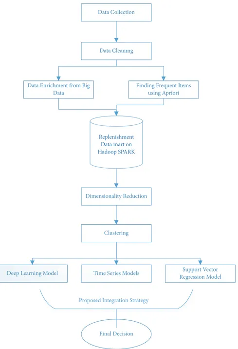
Data Collection
Data Cleaning
Data Enrichment from Big Data
Finding Frequent Items using Apriori Replenishment Data mart on Hadoop SPARK Dimensionality Reduction Clustering
Deep Learning Model Time Series Models Support Vector
Regression Model
Final Decision Proposed Integration Strategy
Figure 1: Flowchart of the proposed system.
as it is marked. This enables faster computation time in which the system disregards poor performing algorithms. The algorithm of the proposed demand forecasting system and the flowchart of the proposed system are given in Algorithm 1 and Figure 1, respectively.
4. Experiment Setup
We use an enhanced dataset which includes SOK Market’s real life sales and stock data with enriched features. The dataset consists of 106 weeks of sales data that includes 7888 distinct products for different stores of SOK Market. On each store, around 1500 products are actively sold while the rest
rarely become active. The forecasting is being performed for each week to predict demand of the following week. Three-fold cross validation methodology is applied for testing data and then decides with the best accurate one of them for the next coming week forecast. This is a common approach making demand forecasting in retail [44]. Furthermore, outside weather information, such as daily temperature and other weather conditions, is joined to the model as new variables. Since it is known that there is a certain correlation between shopping trends and weather conditions at retail in most circumstances [33], we enriched the dataset with the weather information. The dataset also includes mostly sales related features filled from relational legacy data sources.
Given: n is the number of stores, m is the number of products, t is the number of
algorithms in the system and𝐴𝑡is an algorithm with index t.𝑠𝑚,𝑛is the matrix which includes the number of best performing algorithms for each store, and product,𝐵𝑚,𝑛is the matrix which contains the set of blacklist of algorithms for each store, and product, and 𝐹𝑖,𝑗is the matrix which stores final decision of each forecast where i is the number of stores and j is the number of products.
for i=1:n for j=1:m
for k=1:t
if𝐴𝑘is in list𝐵𝑖,𝑗then continue else run𝐴𝑘
Calculate algorithm weight𝑊𝑘 end if
end for for k=1:t
Choice best performing algorithms and locate in{𝑠𝑖,𝑗} end for
for z=1:𝑠𝑖,𝑗 do scaling for𝐴𝑧 end for
Calculate proposed integration strategy, and store in𝐹𝑖,𝑗 end for
end for return all𝐹𝑛,𝑚
Algorithm 1: The algorithm of the proposed demand forecasting system.
Deep learning approach is used to estimate customer demand for each product at each store of SOK Market retail chain. There is also very apparent similarity between products, which are mostly in the same basket in terms of sales trends. For this purpose, Apriori algorithm [4] is utilized to find correlated products of each product. Apriori algorithm is a fast way to find out most associated products which are at the same basket. The most associated product’s sales related features are added to dataset, as well. This takes the advantage of relationships among products with similar sales trends. Addition of associated product of a product and its features enables DL algorithm to learn better within different hidden layers. In summary, it is observed in extensive experiments that enhancements of training dataset with weather data and most associated products sales data made our estimates more powerful with the usage of DL algorithm.
The dataset includes weekly based data of each product at each store for the latest 8 weeks and sales quantities of the last 4 weeks in the same season. Historically, 2 years of data are included for each 5500 stores and 1500 products. Data size is about 875 million records within 155 features. These features include sales quantity, customer return quantity, received product quantities from distribution centers, sales amount, discount amount, receipt counts of a product, customer counts who bought a specific product, sales quantity for each day of week (Monday, Tuesday, etc.), maximum and minimum stock level of each day, average stock level for each week, sales quantity for each hour of the days, and also sales quantities of last 4 weeks of the same season. Since there is a relationship between products which are generally in the same basket, we prepared the same features defined above for
the most associated products, as well. Detailed explanation of the dataset is presented in Table 2.
In Table 2 fields given with square brackets mean that it is an array for each week (Ex. Sales quantity week 0 means sales quantity of current week and sales quantity week 1 is for sales quantity for one week before and so on). Regarding experimental results, taking weekly data for the latest 8 weeks and 4 weeks of the same season at previous year gives more acceptable trends of changes in seasonality.
For DL implementation part, H2O library [31] is used as an open source big data artificial intelligence platform. H2O is a powerful machine learning library and gives us opportunity to implement DL algorithms on Hadoop Spark big data environments. It puts together the power of highly advanced machine learning algorithms and provides to get benefit of truly scalable in-memory processing for Spark big data environment on one or many nodes via its version of Sparkling Water. By the help of in-memory processing capability of Spark technologies, it provides faster parallel platform to utilize big data for business requirements to get maximum benefit. In this study, we use H2O version 3.14.0.2 on 64-bit, 16-core, and 32GB memory machine to observe the power of parallelism during DL modelling while increasing the number of neurons.
A multilayer feedforward artificial neural network (MLFANN) is employed as a deep learning algorithm. MLFANN is trained with stochastic gradient descent using backpropagation. Using gradient descent, each weight is adjusted according to its contribution value to the error. H2O has also advanced features like momentum training, adaptive learning rate, L1 or L2 regularization, rate annealing,
Table 2: Dataset explanation.
Name Description Example
Yearweek Related yearweek, weeks are starting from Monday to Sunday 201801
Store Store number 1234
Product Product Identification Number 1
Product Adjactive Associated product with the product according to apriori algorithm. Most frequent
product at the same basket with a specific product. 2
Stock In Quantity Week[0-8] Stock increase quantity of the product in related week, ex. stock transfer quantityfrom distribution center to store. 50
Return Quantity Week[0-8] Stock return quantity from customers at a specific week and store 20
Sales Quantity Week[0-8] Weekly sales quantity of related product at a specific store 120
Sales Amount Week[0-8] Total sales amount of the product at the customer receipt 2500
Discount Amount Week[0-8] Discount amount of the product if there is any 500
Customer Count Week[0-8] How many customers bought this product at a specific week 30
Receipt Count Week[0-8] Distinct receipt count for related product 20
Sales Quantity Time[9-22] Hourly sales quantity of related product from 9 am to 22 pm. 5
Last4weeks Day[1-7] Total sales of each weekday of last 4 weeks. Total sales of Mondays, Tuesdays. . . etc. 10
Last8weeks Day[1-7] Total sales of each weekday of last 8 weeks. Total sales of Mondays, Tuesdays. . . etc. 10
Max Stock Week[0-8] Maximum stock quantity of related week. 12
Min Stock Week[0-8] Minimum stock quantity of related week 2
Avg Stock Week[0-8] Average stock quantity of related week 5
Sales Quantity Adj Week[0-8] Sales quantity of most associated product 14
Temperature Weekday[1-7] Daily temperature of weekdays. Monday, Tuesday. . . etc. 22
Weekly Avg Temperature[0-8] Average weather temperature of related week. 23
Weather Condition Weekday[1-7] Nominal variable; rainy, snowy, sunny, cloudy etc. Rainy
Sales Quantity Next Week Target variable of our classification problem 25
dropout, and grid search. Gaussian distribution is applied because of the usage of continuous variable as response variable. H2O performs very well in our environment when 3 level hidden layers, 10 nodes each of them, and totally 300 epochs are set as parameters.
After implementing dimension reduction step, K-means is employed as a clustering algorithm. K-means is a greedy and fast clustering algorithm [45] that tries to partition samples into k clusters in which each sample is near to the cluster center. K is selected as 20 because, after several trials and empirical observations, the most even distribution on dataset is reached and divided our dataset into 20 differ-ent clusters for each store. After that part, deep learning algorithm is applied and obtained 20 different DL models for each store. Then, demand forecasting for each product is performed by using its cluster’s model on a store basis. The main reason of using clustering is time and computing lack for DL algorithm. Instead of making modelling for each store, 20 models are generated for each store in product level. Our trials with sample dataset bias difference are less than 2%, so this speed-up is very beneficial and a good option for researchers. The forecasting result of the DL model is transferred into our forecasting system that makes its final decision by considering decisions of 11 forecasting methods including DL model.
Forecasting solutions should be scalable, process large amounts of data, and extract a model from data. Big data
environments using Spark technologies give us opportunity for implementing algorithms with scalability that shares tasks of machine learning algorithms among nodes of parallel architectures. Considering huge amounts of samples and large number of features, even the computational power of parallel architecture is not enough in some of cases. For this reason, dimension reduction is needed for big data applications. In this study, PCA is employed as a feature extraction step.
5. Experimental Results
Forecasting solutions should be scalable, process large amounts of data, and extract a model from data. Big data environments using Spark technologies give us opportunity for implementing algorithms with scalability that shares tasks of machine learning algorithms among nodes of parallel architectures. Considering huge amounts of samples and large number of features, even the computational power of parallel architecture is not enough in some of cases. For this reason, dimension reduction is needed for big data applications. In this study, PCA is employed as a feature extraction step.
SOK Market sells 21 different groups of items. We assess the performance of the proposed forecasting system on group basis as shown in Table 3. Table 3 shows MAPE (Mean Abso-lute Percentage Error) of integration strategies (S1) and (S2)
T a b le 3: D em an d fo recas tin g im p ro vem en ts p er p ro d u ct gr o u p . Pro d u ct Gr ou p s Me th o d I wi th o u t P ro p o se d In tegra tio n Stra teg y (𝑆1 ) MAP E Me th o d II wi th P ro p os ed In tegra tio n Stra teg y (𝑆2 ) MAP E Prop o se d In te gr at io n Stra teg y w ith Deep Le ar n in g (𝑆𝐷 ) MAP E Pe rc en ta ge Succes s Ra te 𝑃1 =( 𝑆1 −𝑆 2 )/𝑆2 Pe rc en ta ge Succes s Ra te 𝑃2 =( 𝑆1 −𝑆 𝐷 )/𝑆𝐷 Im p ro vem en t 𝐷=𝑃 2 −𝑃 1 B ab y P ro d uc ts 0.51 57 0.3 08 1 0.29 27 4 0.26% 43 .2 5% 2.99 % B ak er y P ro d uc ts 0.3 4 82 0.2059 0.1 96 6 4 0 .8 5% 43 .5 2% 2.67% B ev erag e 0.3 71 4 0.2 31 6 0.2207 37 .6 4 % 4 0.58 % 2.9 4% B is cui t-Cho co la te 0 .3 358 0 .207 7 0 .1 97 7 38 .1 4 % 4 1.13% 2.9 9% B reakfas t P ro d u ct s 0 .4 4 43 0 .27 70 0 .26 61 37 .6 5% 4 0.11% 2.45% C anned -P as te-S auces 0.3 83 6 0.2 30 9 0.21 98 39 .8 0% 42.6 9% 2.8 9% Chees e 0 .3 95 3 0 .2 457 0 .2 34 5 37 .8 4 % 4 0.6 8% 2.8 4% Clea nin g P ro d uc ts 0.45 6 0 0.279 1 0.26 50 38 .79 % 41 .8 9% 3.1 0 % C o sm etic s P ro d u ct s 0 .5 39 7 0 .3 26 6 0 .3 14 8 39 .4 9% 4 1.67% 2.1 9% Deli M ea ts 0 .42 4 2 0 .26 02 0 .2 4 88 38 .6 5% 4 1.3 6 % 2.70% E d ib le Oils 0.4 0 6 0 0.2299 0 .221 5 43.3 6 % 4 5.4 5% 2.0 9% H o us eho ld G o o d s 0 .57 13 0 .3 65 6 0 .35 35 36.01% 38 .13% 2.12% Ic e C re am -F ro zen 0 .5 012 0 .3 25 5 0 .3 10 6 35.05% 38 .0 3% 2.9 8% L egumes -P as ta-S o u p 0.3 85 0 0.2 39 7 0.226 9 37 .7 4 % 4 1. 07% 3.3 3% N u ts -C hi ps 0.3 31 6 0 .20 49 0 .1 96 6 38 .20% 4 0.7 1% 2.51% P o ul tr y E ggs 0.421 9 0.2 527 0.2 4 03 4 0 .1 1% 43 .0 4% 2.9 4 % R ead y M eals 0.4 61 3 0.26 10 0.2 520 43 .42% 45.3 6% 1. 94 % Red M ea t 0 .2 51 4 0 .16 16 0 .15 32 35.7 1% 39 .0 6% 3.35% T ea-C o ff ee P ro d u ct s 0 .4 34 7 0 .26 50 0 .2 53 5 39 .0 4 % 4 1.6 8% 2.6 4% T extile P ro d u ct s 0 .5 418 0 .3 0 4 8 0 .29 0 7 43.7 4 % 4 6.3 4 % 2.6 0% T o bacco P ro d uc ts 0.3 79 1 0.2 37 8 0.2290 37 .29 % 39 .6 1% 2.3 2% A ver ag e 0 .4 23 8 0 .2 58 2 0 .2 46 9 38.9 9% 41 .6 8% 2.6 9%
1.00 0.75 0.50 0.25 0.00 MAPE PRODUCT GROUPS B ab y P ro d uc ts B ak er y P ro d uc ts B ev erag e B is cui t–Cho co la te B re akfast P ro d uc ts C anned–P ast e–Sa uces Ch eese Cle anin g P ro d uc ts C osmetics P ro d uc ts D eli M ea ts Edib le Oils H o us eho ld G o o d s Ice Cr ea m–F ro zen L egumes–P ast a–S o u p N u ts–Chi ps P o ul tr y–E gg s Red M ea t Re ad y M eals T ea–C o ff ee P ro d uc ts T extile P ro d uc ts T o bacco P ro d uc ts
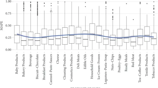
Figure 2: MAPE distribution according to product groups with S1integration strategy.
in columns 2 and 3. The average percentage forecasting errors of strategies (S1) and (S2) are 0.42 and 0.26, respectively. As it can be seen from Table 3, the percentage success rate of (S2) in accordance with (S1) is represented in column 5. The current integration strategy (S2) provides 38.99% improvement over the first integration strategy (S1) average. In some product groups like Textile Products, the error rate is reduced from 0.54 to 0.31 with 43.74% enhancement in MAPE.
With this work, a further improvement is obtained by utilizing DL model compared to the usage of just 10 algorithms which are based on forecasting strategy. Column 4 of Table 3 demonstrates MAPEs of 21 different groups of products after the addition of DL model. After the inclusion of DL model into the proposed system, we observed around 2% to 3.4% increase in demand forecast accuracies in some of product groups. The error rates of some product groups like “baby products,” “cosmetic products,” and “household goods” are usually higher than others, since these product groups do not have continuous demand by consumers. For example, the error rate for “household goods” group is 0.35 while the error rate for “red meat” group is 0.15. The error rates in food products are usually lower, since customers consider their daily consumption regularly to buy these products. However, the error rates are higher in baby, textile, and household goods. Customers buy products from these groups depending on whether they like the product or not selectively. In addition, the prices of goods in these groups and promotion effects are usually high relative to the prices of goods in other groups.
Moreover, it is observed that the top benefitted product groups for Method I accomplishes over 40% success rate on Baby Products, Bakery Products, Edible Oils, Poultry Eggs, Ready Meals, and Textile Products when the column
of percentage success rate is analyzed. The common point of these groups is that each one of them is being consumed by a specific customer segment, regularly. For instance, baby products group is being chosen by families who have kids; Edible Oils, Poultry Eggs, and Bakery Products are being preferred by frequently and continuously shopping customer segments; and Ready Meals are being preferred by mostly bachelor, single, and working consumers, etc. Furthermore, the inclusion of DL into the forecasting system indicates that some other consuming groups (for example, Cleaning Products, Red Meats, and Legumes Pasta Soup) exhibit better performance than the others with additional over 3%.
Figure 2 shows the box plots of mean percentage errors (MAPE) for each group of products after application of (S1) integration strategy. The box plots enable us to analyze distributional characteristics of forecasting errors for product groups. As it can be seen from the figure, there are different medians for each product group. Thus, the forecasting errors are usually dissimilar for different products groups. The interquartile range box represents the middle 50% of scores in data. The lengths of interquartile range boxes are usually very tall. This means that there are quite number of different prediction errors within products of a given group.
Figure 3 presents the box plots of MAPEs of the proposed forecasting system that apply proposed integration approach (S2) which combines the predictions of 10 different forecast-ing algorithms.
Figure 4 shows after adding DL to our system results. The lengths of interquartile range boxes are narrower when compared to the ones in Figures 2 and 3. This means that the distribution of forecasting errors is less than Figures 2 and 3. Finally, the integration of DL into the proposed forecasting system generates results that are more accurate.
1.00 0.75 0.50 0.25 0.00 MAPE PRODUCT GROUPS B ab y P ro d uc ts B ak er y P ro d uc ts B ev erag e B is cui t–Cho co la te B re akfast P ro d uc ts C anned–P ast e–Sa uces Ch eese Cle anin g P ro d uc ts C osmetics P ro d uc ts D eli M ea ts Edib le Oils H o us eho ld G o o d s Ice Cr ea m–F ro zen L egumes–P ast a–S o u p N u ts–C hi ps P o ul tr y–E gg s Red M ea t Re ad y M eals T ea–C o ff ee P ro d uc ts T extile P ro d uc ts T o bacco P ro d uc ts
Figure 3: MAPE distribution according to product groups with S2integration strategy.
1.00 0.75 0.50 0.25 0.00 MAPE PRODUCT GROUPS B ab y P ro d uc ts B ak er y P ro d uc ts B ev erag e B is cui t–Cho co la te B re akfast P ro d uc ts C anned–P ast e–Sa uces Ch eese Cle anin g P ro d uc ts C osmetics P ro d uc ts D eli M ea ts Edib le Oils H o us eho ld G o o d s Ice Cr ea m–F ro zen L egumes–P ast a–S o u p N u ts–Chi ps P o ul tr y–E gg s Red M ea t Re ad y M eals T ea–C o ff ee P ro d uc ts T extile P ro d uc ts T o bacco P ro d uc ts
Figure 4: MAPE distribution according to product groups after deep learning algorithms.
For example, for the (S1) integration strategy in Baby Products product group MAPE distribution for the 1st quar-tile of data 5 is observed between 0% and 23%, for 2nd quarquar-tile between 23% and 48%, and for 3rd and 4th between 48% and 75% in Figure 2. After applying integration strategy for Baby Products product group, MAPE distribution becomes 0%–16% for the 1st quartile, 16%–30% for the 2nd quartile of the data, and 30%–50% for the rest. This gives around 8% improvement for the first quartile, from 8% to 18% enhancement for the second quartile, and from 18% to 25% advancement for the rest of the data according to boundaries
differences. Median of MAPE distribution is analyzed as 48%. After applying the proposed integration strategy, it is observed as 27%, which means 21% improvement. Approx-imately 1%-3% enhancement is observed for each quartile of the data with the inclusion of deep learning strategy in Figure 4.
For Cleaning Products, similar improvements are observed with the others; for integration strategy MAPE distribution of the 1st quartile of data is observed between 0% and 19%, for the 2nd quartile it is between 19% and 40%, and for the rest of data it is observed between 40% and
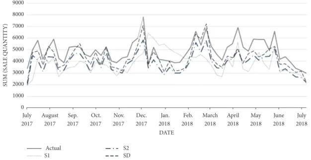
SU M (SALE Q U ANTIT Y) DATE 9000 8000 7000 6000 5000 4000 3000 2000 1000 0
July August Sep. Oct. Nov. Dec. Jan. Feb. March April May June July
Actual S1
S2 SD
2017 2017 2017 2017 2017 2017 2018 2018 2018 2018 2018 2018 2018
Figure 5: Accuracy comparison among integration strategies for one sample product group.
73% in Figure 2. After performing the proposed integration strategy for Cleaning Products, MAPE distribution becomes 0%–10% for the 1st quartile of data, 10%–17% for the 2nd quartile, and 27%–43% for the 3rd and 4th quartiles together. Improvements are observed as follows: 9% for the 1st quartile, from 9% to 13% for the 2nd quartile, and from 13% to 20% for the rest of the data at boundaries. After implementation of the integration strategy for the 1st and 2nd quartiles, the system advancement is observed as 2%, and for the 3rd and 4th quartiles it is %3, respectively. Briefly, integration strategy improvement is remarkable for each product group and consolidation of DL to the proposed integration strategy advances results between almost 2% and 3%, additionally.
In Figure 5, the accuracy comparison among integration strategies of one of the best performing sample groups is presented during 1-year period. Particularly, Christmas and other seasonality effects can be seen very clearly at Figure 5 and integration strategy with DL (SD) is performing with the best accuracy.
It is hard to compare the performance of our proposed system with the other studies because of the lack of works with similar combinations of deep learning approach, the proposed decision integration strategies, and different learn-ing algorithms for demand forecastlearn-ing process. Another difficulty is the deficiency of real-life dataset similar to SOK dataset in order to compare the state-of-art studies. Although the results of proposed system are given in this study, we also report the results of a number of research works here on demand forecasting domain. A greedy aggregation-decomposition method has solved a real-world intermittent demand forecasting problem for a fashion retailer in Sin-gapore [46]. They report 5.9% MAPE success rate with a small dataset. Authors compare different approaches such as statistical model, winter model, and radius basis function neural network (RBFNN) with SVM for demand forecasting process in [47]. As a result, they conclude the study by the
fact that the success of SVM algorithm surpasses others with around 7.7% enhancement at average MAPE results level. A novel demand forecasting model called SHEnSVM (Selective and Heterogeneous Ensemble of Support Vec-tor Machines) is proposed in [48]. The proposed model presents that the individual SVMs are trained by different samples generated by bootstrap algorithm. After that, genetic algorithm is employed for retrieving the best individual combination schema. They report 10% advancement with SVM algorithm and 64% MAPE improvement. They only employ beer data with 3 different brands in their experiments. Tugba Efendigil et al. propose a novel forecasting mechanism which is modeled by artificial intelligence approaches in [49]. They compared both artificial neural networks and adaptive network-based fuzzy inference system techniques to manage the fuzzy demand with incomplete information. They reached around 18% MAPE rates for some products during their experiments.
6. Conclusion
In retail industry, demand forecasting is one of the main problems of supply chains to optimize stocks, reduce costs, and increase sales, profit, and customer loyalty. To overcome this issue, there are several methods such as time series analysis and machine learning approaches to analyze and learn complex interactions and patterns from historical data. In this study, there is a novel attempt to integrate the 11 different forecasting models that include time series algo-rithms, support vector regression model, and deep learning method for demand forecasting process. Moreover, a novel decision integration strategy is developed by drawing inspi-ration from the ensemble methodology, namely, boosting. The proposed approach considers the performance of each model in time and combines the weighted predictions of the best performing models for demand forecasting process. The
proposed forecasting system is tested and carried out real life data obtained from SOK Market retail chain. It is observed that the inclusion of different learning algorithms except time series models and a novel integration strategy advanced the performance of demand forecasting system. To the best of our knowledge, this is the very first attempt to consolidate deep learning methodology, SVR algorithm, and different time series methods for demand forecasting systems. Fur-thermore, the other novelty of this work is the adaptation of boosting ensemble strategy to the demand forecasting model. In this way, the final decision of the proposed system is based on the best algorithms of the week by gaining more weight. This makes our forecasts more reliable with respect to the trend changes and seasonality behaviors. Moreover, the proposed approach performs very well integrating with deep learning algorithm on Spark big data environment. Dimension reduction process and clustering methods help to decrease time consuming with less computing power during deep learning modelling phase. Although a review of some of similar studies is presented in Section 5, as it is expected, it is very difficult to compare the results of other studies with ours because of the use of different datasets and methods. In this study, we compare results of three models where model one selects the best performing forecasting method depending on its success on previous period with 42.4% MAPE on average. The second model with the novel integration strategy results in 25.8% MAPE on average. The last model with the novel integration strat-egy enhanced with deep learning approach provides 24.7% MAPE on average. As a result, the inclusion of deep learning approach into the novel integration strategy reduces average prediction error for demand forecasting process in supply chain.
As a future work, we plan to enrich the set of features by gathering data from other sources like economic studies, shopping trends, social media, social events, and location based demographic data of stores. New variety of data sources contributions to deep learning can be observed. One more study can be done to determine the hyperpa-rameters for deep learning algorithm. In addition, we also plan to use other deep learning techniques such as con-volutional neural networks, recurrent neural networks, and deep neural networks as learning algorithms. Furthermore, our another objective is to use heuristic methods MBO (Migrating Birds Optimization) and other related algorithms [50] to optimize some of coefficients/weights which were determined empirically by trial-and-error like taking 30% percent of the best performing methods in our current system.
Data Availability
This dataset is private customer data, so the agreement with the organization SOK does not allow sharing data.
Conflicts of Interest
The authors declare that there are no conflicts of interest regarding the publication of this article.
Acknowledgments
This work is supported by OBASE Research & Development Center.
References
[1] P. J. McGoldrick and E. Andre, “Consumer misbehaviour: promiscuity or loyalty in grocery shopping,” Journal of Retailing
and Consumer Services, vol. 4, no. 2, pp. 73–81, 1997.
[2] D. Grewal, A. L. Roggeveen, and J. Nordf¨alt, “The Future of Retailing,” Journal of Retailing, vol. 93, no. 1, pp. 1–6, 2017. [3] E. T. Bradlow, M. Gangwar, P. Kopalle, and S. Voleti, “the role
of big data and predictive analytics in retailing,” Journal of
Retailing, vol. 93, no. 1, pp. 79–95, 2017.
[4] J. Han, M. Kamber, and J. Pei, Data Mining: Concepts and
Techniques, Morgan Kaufmann Publishers, USA, 2013.
[5] R. Hyndman and G. Athanasopoulos, Forecasting: Principles
and Practice, OTexts, Melbourne, Australia, 2018, http://otexts
.org/fpp2/.
[6] C. C. Pegels, “Exponential forecasting: some new variations,”
Management Science, vol. 12, pp. 311–315, 1969.
[7] E. S. Gardner, “Exponential smoothing: the state of the art,”
Journal of Forecasting, vol. 4, no. 1, pp. 1–28, 1985.
[8] D. Gujarati, Basic Econometrics, Mcgraw-Hill, New York, NY, USA, 2003.
[9] J. D. Croston, “Forecasting and stock control for intermittent demands,” Operational Research Quarterly, vol. 23, no. 3, pp. 289–303, 1972.
[10] T. R. Willemain, C. N. Smart, J. H. Shockor, and P. A. DeSautels, “Forecasting intermittent demand in manufacturing: a compar-ative evaluation of Croston’s method,” International Journal of
Forecasting, vol. 10, no. 4, pp. 529–538, 1994.
[11] A. Syntetos, Forecasting of intermittent demand, Brunel Univer-sity, 2001.
[12] A. A. Syntetos and J. E. Boylan, “The accuracy of intermittent demand estimates,” International Journal of Forecasting, vol. 21, no. 2, pp. 303–314, 2005.
[13] R. H. Teunter, A. A. Syntetos, and M. Z. Babai, “Intermittent demand: linking forecasting to inventory obsolescence,”
Euro-pean Journal of Operational Research, vol. 214, no. 3, pp. 606–
615, 2011.
[14] R. J. Hyndman, R. A. Ahmed, G. Athanasopoulos, and H. L. Shang, “Optimal combination forecasts for hierarchical time series,” Computational Statistics & Data Analysis, vol. 55, no. 9, pp. 2579–2589, 2011.
[15] R. Fildes and F. Petropoulos, “Simple versus complex selection rules for forecasting many time series,” Journal of Business
Research, vol. 68, no. 8, pp. 1692–1701, 2015.
[16] C. Li and A. Lim, “A greedy aggregation–decomposition method for intermittent demand forecasting in fashion retail-ing,” European Journal of Operational Research, vol. 269, no. 3, pp. 860–869, 2018.
[17] F. Turrado Garc´ıa, L. J. Garc´ıa Villalba, and J. Portela, “Intelli-gent system for time series classification using support vector machines applied to supply-chain,” Expert Systems with
Appli-cations, vol. 39, no. 12, pp. 10590–10599, 2012.
[18] G. Song and Q. Dai, “A novel double deep ELMs ensemble system for time series forecasting,” Knowledge-Based Systems, vol. 134, pp. 31–49, 2017.
[19] O. Araque, I. Corcuera-Platas, J. F. S´anchez-Rada, and C. A. Iglesias, “Enhancing deep learning sentiment analysis with ensemble techniques in social applications,” Expert Systems with
Applications, vol. 77, pp. 236–246, 2017.
[20] H. Tong, B. Liu, and S. Wang, “Software defect prediction using stacked denoising autoencoders and twostage ensemble learning,” Information and Software Technology, vol. 96, pp. 94– 111, 2018.
[21] X. Qiu, Y. Ren, P. N. Suganthan, and G. A. J. Amaratunga, “Empirical mode decomposition based ensemble deep learning for load demand time series forecasting,” Applied Soft
Comput-ing, vol. 54, pp. 246–255, 2017.
[22] Z. Qi, B. Wang, Y. Tian, and P. Zhang, “When ensemble learning meets deep learning: a new deep support vector machine for classification,” Knowledge-Based Systems, vol. 107, pp. 54–60, 2016.
[23] Y. Bengio, A. Courville, and P. Vincent, “Representation learn-ing: a review and new perspectives,” IEEE Transactions on
Pattern Analysis and Machine Intelligence, vol. 35, no. 8, pp.
1798–1828, 2013.
[24] G. E. Hinton, S. Osindero, and Y. Teh, “A fast learning algorithm for deep belief nets,” Neural Computation, vol. 18, no. 7, pp. 1527– 1554, 2006.
[25] Y. Bengio, “Practical recommendations for gradient-based training of deep architectures,” in Neural Networks: Tricks of the
Trade, vol. 7700 of Lecture Notes in Computer Science, pp. 437–
478, Springer, Berlin, Germany, 2nd edition, 2012.
[26] Y. LeCun, Y. Bengio, and G. Hinton, “Deep learning Review,”
International Journal of Business and Social Science, vol. 3, 2015.
[27] S. Kim, Z. Yu, R. M. Kil, and M. Lee, “Deep learning of support vector machines with class probability output networks,” Neural
Networks, vol. 64, pp. 19–28, 2015.
[28] P. J. Brockwell and R. A. Davis, Time Series: Theory And
Methods, Springer Series in Statistics, New York, NY, USA, 1989.
[29] V. N. Vapnik, Statistical Learning Theory, Wiley- Interscience, New York, NY, USA, 1998.
[30] S. Haykin, Neural Networks and Learning Machines, Macmillan Publishers Limited, New Jersey, NJ, USA, 2009.
[31] A. Candel, V. Parmar, E. LeDell, and A. Arora, Deep Learning
with H2O, United States of America, 2018.
[32] K. Keerthi Vasan and B. Surendiran, “Dimensionality reduction using principal component analysis for network intrusion detection,” Perspectives in Science, vol. 8, pp. 510–512, 2016. [33] L. Rokach, “Ensemble-based classifiers,” Artificial Intelligence
Review, vol. 33, no. 1-2, pp. 1–39, 2010.
[34] R. Polikar, “Ensemble based systems in decision making,” IEEE
Circuits and Systems Magazine, vol. 6, no. 3, pp. 21–45, 2006.
[35] Reid. Sam, A review of heterogeneous ensemble methods, Depart-ment of Computer Science, University of Colorado at Boulder, 2007.
[36] D. Gopika and B. Azhagusundari, “An analysis on ensem-ble methods in classification tasks,” International Journal of
Advanced Research in Computer and Communication Engineer-ing, vol. 3, no. 7, pp. 7423–7427, 2014.
[37] Y. Ren, L. Zhang, and P. N. Suganthan, “Ensemble classification and regression-recent developments, applications and future directions,” IEEE Computational Intelligence Magazine, vol. 11, no. 1, pp. 41–53, 2016.
[38] U. G. Mangai, S. Samanta, S. Das, and P. R. Chowdhury, “A survey of decision fusion and feature fusion strategies for
pattern classification,” IETE Technical Review, vol. 27, no. 4, pp. 293–307, 2010.
[39] M. Wo´zniak, M. Gra˜na, and E. Corchado, “A survey of multiple classifier systems as hybrid systems,” Information Fusion, vol. 16, no. 1, pp. 3–17, 2014.
[40] G. Tsoumakas, L. Angelis, and I. Vlahavas, “Selective fusion of heterogeneous classifiers,” Intelligent Data Analysis, vol. 9, no. 6, pp. 511–525, 2005.
[41] Y. Freund and R. E. Schapire, “A decision-theoretic generaliza-tion of on-line learning and an applicageneraliza-tion to boosting,” Journal
of Computer and System Sciences, vol. 55, no. 1, part 2, pp. 119–
139, 1997.
[42] S. Chopra and P. Meindl, Supply Chain Management: Strategy,
Planning, and Operation, Prentice Hall, 2004.
[43] G. Kushwaha, “Operational performance through supply chain management practices,” International Journal of Business and
Social Science, vol. 217, pp. 65–77, 2012.
[44] G. E. Box, G. M. Jenkins, G. Reinsel, and G. M. Ljung,
Time Series Analysis: Forecasting and Control, Wiley Series in
Probability and Statistics, John Wiley & Sons, Hoboken, NJ, USA, 5th edition, 2015.
[45] W.-L. Zhao, C.-H. Deng, and C.-W. Ngo, “k-means: a revisit,”
Neurocomputing, vol. 291, pp. 195–206, 2018.
[46] C. Li and A. Lim, “A greedy aggregation-decomposition method for intermittent demand forecasting in fashion retailing,”
Euro-pean Journal of Operational Research, vol. 269, no. 3, pp. 860–
869, 2018.
[47] L. Yue, Y. Yafeng, G. Junjun, and T. Chongli, “Demand forecast-ing by usforecast-ing support vector machine,” in Proceedforecast-ings of the Third
International Conference on Natural Computation (ICNC 2007),
pp. 272–276, Haikou, China, August 2007.
[48] L. Yue, L. Zhenjiang, Y. Yafeng, T. Zaixia, G. Junjun, and Z. Bofeng, “Selective and heterogeneous SVM ensemble for demand forecasting,” in Proceedings of the 2010 IEEE 10th
Inter-national Conference on Computer and Information Technology (CIT), pp. 1519–1524, Bradford, UK, June 2010.
[49] T. Efendigil, S. ¨On¨ut, and C. Kahraman, “A decision support system for demand forecasting with artificial neural networks and neuro-fuzzy models: a comparative analysis,” Expert
Sys-tems with Applications, vol. 36, no. 3, pp. 6697–6707, 2009.
[50] E. Duman, M. Uysal, and A. F. Alkaya, “Migrating birds opti-mization: a new metaheuristic approach and its performance on quadratic assignment problem,” Information Sciences, vol. 217, pp. 65–77, 2012.
Hindawi www.hindawi.com Volume 2018
Mathematics
Journal of Hindawi www.hindawi.com Volume 2018 Mathematical Problems in Engineering Applied Mathematics Hindawi www.hindawi.com Volume 2018Probability and Statistics Hindawi
www.hindawi.com Volume 2018
Hindawi
www.hindawi.com Volume 2018
Mathematical PhysicsAdvances in
Complex Analysis
Journal ofHindawi www.hindawi.com Volume 2018
Optimization
Journal of Hindawi www.hindawi.com Volume 2018 Hindawi www.hindawi.com Volume 2018 Engineering Mathematics International Journal of Hindawi www.hindawi.com Volume 2018 Operations Research Journal of Hindawi www.hindawi.com Volume 2018Function Spaces
Abstract and Applied AnalysisHindawi www.hindawi.com Volume 2018 International Journal of Mathematics and Mathematical Sciences Hindawi www.hindawi.com Volume 2018
Hindawi Publishing Corporation
http://www.hindawi.com Volume 2013 Hindawi www.hindawi.com
World Journal
Volume 2018 Hindawiwww.hindawi.com Volume 2018Volume 2018