A- APPLIED SCIENCES AND ENGINEERING
2019, 20(3), pp. 346 - 364, DOI: 10.18038/estubtda.540384
RISK-AVERSE STOCHASTIC ORIENTEERING PROBLEMS Özlem ÇAVUŞ 1,*
1 Department of Industrial Engineering, Faculty of Engineering, Bilkent University, Ankara, Turkey ABSTRACT
In this study, we consider risk-averse orienteering problems with stochastic travel times or stochastic rewards. In risk-neutral orienteering problems, the objective is generally to maximize the expected total reward of visited nodes. However, due to uncertain travel times or uncertain rewards, the dispersion in total reward collected may be large, which necessitates an approach that minimizes the dispersion (risk) in addition to maximizing the expected total reward. To handle this, for the orienteering problems with stochastic travel times or stochastic rewards, we suggest two different formulations with an objective of coherent measures of risk. For both problems, we conduct an experimental study using two different coherent measures of risk, which have been extensively used in the literature, and compare the results. The computational results show that, in both models suggested and under both risk measures used, the decision maker is able to obtain a tour with expected total reward being close to the expected total reward of risk-neutral solution, however with a significant decrease in the standard deviation of total reward.
Keywords: Stochastic orienteering problem, Risk-averse optimization, Coherent measures of risk, Mean conditional
value-at-risk, Mean semi-deviation
1. INTRODUCTION
Orienteering Problem (OP) aims to find a tour that starts at a depot node, visits each node in a subset of all nodes exactly once and ends at the depot node. Different from the travelling salesman problem, not all the nodes are required to be visited, the tour should be completed within a given time limit, and each node has an associated reward. The objective of OP is to maximize the total reward collected from the visited nodes. The orienteering problem is first introduced by Tsiligirides [1] and Golden et al. [2], since then has been studied extensively in the literature. The reader is referred to the survey papers Vansteenwegen et al. [3] and Gunawan et al. [4] for details.
The OP has many different applications in many different areas, e.g. logistics, traffic problems and defense industry. In the literature, there is a large number of studies focusing on deterministic OP, however, the number of studies on stochastic variant is limited. In deterministic OP, the profit and service time of each node and the travel times between the nodes are assumed to be deterministic. However, this assumption may not be realistic for some real life applications, for example, in a logistics system, the congestion on the road network leads to random travel times or customers may have stochastic demands.
The stochastic OP is first introduced by Teng et al. [5], where a two-stage stochastic programming formulation with stochastic travel and service times is proposed. The tour is constructed in the first stage before observing the uncertainty, and after the uncertainty is resolved, the time of the tour in excess of the time limit is computed in the second stage. The objective is to maximize the expected profit of the tour, which is total reward of the tour minus the expected penalty of exceeding the time limit. A two-stage problem with stochastic travel and service times is also considered by Campbell et al. [6], however, with different penalty cost definition. A penalty is incurred if a customer in the first stage tour is not visited due to resolved uncertainty. Tang and Miller-Hooks [7] suggest a risk-averse orienteering model with stochastic service times, where risk-aversion is modeled by a chance constraint ensuring that the
probability of the tour not being completed within the time limit does not exceed a threshold probability. Differently, Ilhan et al. [8] study the case of stochastic rewards and propose a model maximizing the probability that the collected total reward will exceed a target level. This model constitutes a risk-averse formulation where risk-aversion is controlled by changing the target level.
Most of the studies on stochastic OP consider only stochastic travel times. Evers et al. [9] propose a two-stage stochastic programming model where the tour constructed in the first stage can be aborted in the second stage before reaching the depot node due to random travel times. The objective is to
maximize the expected total reward of visited nodes. A similar model is suggested by Shang et al.
[10], however with less number of variables and constraints. A chance constrained model with
stochastic travel times is proposed by Varakantham and Kumar [11]. With chance constraint, the
probability that the tour will not be completed within the time limit is forced to be less than some threshold. Dolinskaya et al. [12] propose a dynamic OP with stochastic travel times, where the uncertainty is resolved gradually and the tour is constructed dynamically based on resolved
uncertainty. All these studies consider time independent stochastic travel times. On the other hand, in
Hoong et al. [13], random travel times are assumed to be time dependent. Here, the travel time from
node a to node b depends on the arrival time at node a. Additionally, the decision maker is supposed to be risk-aware and this is taken into account by maximizing total expected utilities of the visited nodes subject to a chance constraint which ensures the tour will be completed within the time limit
with at least a threshold probability. Varakantham et al. [14] extend the study in [11] by considering
time dependent stochastic travel times. Verbeeck et al. [15] also work on an OP with stochastic time dependent travel times and with time windows.
A different version of OP, which has an application in pharmaceutical industry, is considered by Zhang et al. [16]. In that problem context, the sales representatives visit doctors and the time that a sales representative waits at the office of a doctor before seeing him/her, called as waiting time, is assumed to
be random. The problem is modeled as a two-stage stochastic programing model with time windows.
The tour is constructed in the first stage. In the second stage, there are two different recourse actions: a doctor in the tour can be skipped if the representative cannot arrive within the time window of doctor or the representative may renege from or balk the queue if the queue at the doctor is long upon arrival. The objective is to maximize the expected total reward of the tour. This study is extended in [17] by allowing the routing and queuing decisions to be made dynamically based on the realized waiting times.
The literature on the stochastic OP assumes, in general, the decision maker is risk-neutral. Therefore, there is a very limited number of studies focusing on risk-averse decision makers. The risk-averse orienteering studies in the literature can be categorized into three groups based on the modeling approach of the risk-aversion: (i) using probabilistic objective functions [8], (ii) using chance constraints [7], [11], [13], (iii) using utility functions [13]. However, chance constraints are in general nonconvex and additionally may ignore the deviation of the extreme losses (or costs) and the utility functions are difficult to interpret (see, for instance, Shapiro et al. [18]). A modern approach in the literature to model risk-aversion is to use coherent measures of risk. The coherent measures of risk are first introduced by Artzner et al. [19] and the theoretical properties of the stochastic optimization problems with an objective of coherent measure of risk are studied in Ruszczynski and Shapiro [20]-[21].
In general, the objective in a risk-neutral stochastic OP is to maximize the expected total reward of the visited nodes. However, due to the uncertainty in the travel times or the rewards of the nodes, the deviation in the total reward collected may be large. In this study, we do not only aim to maximize the expected total reward of visited nodes but also to minimize the dispersion of total reward. Therefore, the decision maker is assumed to be risk-averse and we use coherent measures of risk to model the risk-aversion. To the best of our knowledge, this is the first study considering coherent measures of risk in OP framework. We focus on two versions of the problem: (i) with stochastic rewards and (ii) with stochastic travel times. For both problems, we propose a stochastic programming model with an
objective of coherent measure of risk. We then use two different coherent measures of risk, which are extensively used in the literature: mean conditional-value-at risk (mean-CVaR) and mean semi-deviation. For both orienteering problems with different risk measures, we provide numerical results on different levels of risk-aversion.
The presentation of the paper is as follows: In Section 2, we briefly explain the concept of coherent measures of risk and provide the definitions of the risk measures considered in the computational results. We introduce our mathematical models in Section 3 and present the numerical results in Section 4. Section 5 is devoted to the concluding remarks.
2. COHERENT MEASURES OF RISK
The concept of coherent measures of risk is first introduced by Artzner et al. [19]. In this section, we briefly explain the axiomatic properties of these risk measures and provide the definitions of the measures of risk we consider in our computational results.
Let (Ω, ℱ, 𝑃) be a probability space where is Ω the sample space, ℱ is sigma algebra of the subsets
of Ω, and 𝑃 is a probability distribution on Ω. In this study, we assume that Ω is finite. Also, let 𝒵 =
ℒ𝑞(Ω, ℱ, 𝑃) be the space of 𝑞-integrable random costs (for which lower values are preferable) for 𝑞 ≥
1 and 𝑝𝜔 be the probability of elementary event 𝜔 ∈ Ω. A risk measure 𝜌: 𝒵 → ℝ is called coherent if
it satisfies the following four axioms [19]:
A1. (Convexity) 𝜌(𝜆𝑋 + (1 − 𝜆)𝑌) ≤ 𝜆𝜌(𝑋) + (1 − 𝜆)𝜌(𝑌) for all 𝜆 ∈ (0,1), 𝑋, 𝑌 ∈ 𝒵, A2. (Monotonicity) If 𝑋(𝜔) ≤ 𝑌(𝜔) for all 𝜔 ∈ Ω then 𝜌(𝑋) ≤ 𝜌(𝑌) for all 𝑋, 𝑌 ∈ 𝒵, A3. (Translation Invariance) 𝜌(𝛾 + 𝑋) = 𝛾 + 𝜌(𝑋) for all 𝛾 ∈ ℝ, 𝑋 ∈ 𝒵,
A4. (Positive Homogeneity) 𝜌(𝛽𝑋) = 𝛽𝜌(𝑋) for all 𝛽 ≥ 0, 𝑋 ∈ 𝒵.
It can be easily shown that the convexity and positive homogeneity axioms together result in subadditivity property:
A5. (Subadditivity) 𝜌(𝑋 + 𝑌) ≤ 𝜌(𝑋) + 𝜌(𝑌) for all 𝑋, 𝑌 ∈ 𝒵.
All these axioms have rational interpretations. Subadditivity (or convexity) axiom implies that
diversification decreases the risk. If a random cost 𝑋 is smaller than or equal to a random cost 𝑌 for
each elementary event 𝜔 ∈ Ω, then we expect the risk of 𝑋 to be smaller than or equal to the risk of 𝑌. This is what monotonicity axiom implies. Translation invariance axiom states that if a random cost is increased by a constant then the risk of it will increase by the same amount. Finally, the constant 𝛽 in positive homogeneity axiom can be interpreted as a currency exchange rate, implying that it does not matter in which currency the risk is computed.
In this study, we use two different coherent measures of risk: mean-CVaR and first-order mean semi-deviation.
Conditional value-at-risk (CVaR) is introduced by Rockafellar and Uryasev [22] and its definition is
extended to any general distribution in [23]. Given an atomless random cost 𝑋, CVaR of 𝑋 at
confidence level 𝛼 ∈ (0,1), denoted as CVaR𝛼(𝑋), is defined as:
CVaR𝛼(𝑋) = 𝔼[𝑋|𝑋 ≥ VaR𝛼(𝑋)],
where VaR𝛼(𝑋) = inf{𝑥: ℙ(𝑋 ≤ 𝑥) ≥ 𝛼}. Note that, for an atomless random cost 𝑋, CVaR𝛼(𝑋) is the
conditional expectation of the values of 𝑋 exceeding value-at-risk (VaR) at level 𝛼, that is VaR𝛼(𝑋).
CVaR𝛼(𝑋) = inf {𝜂 + 1
1−𝛼𝔼[(𝑋 − 𝜂)+]: 𝜂 ∈ ℝ}, (1)
where (𝑎)+= max{𝑎, 0} for 𝑎 ∈ ℝ and the infimum is attained at 𝜂∗=VaR𝛼(𝑋). As 𝛼 increases in
CVaR, the decision maker becomes more risk-averse.
If the sample space Ω is finite then the expression in (1) can be written as the following linear program (see [23]): min 𝜂 + 1 1 − 𝛼∑ 𝑝𝜔𝑧𝜔 𝜔∈Ω (2) s.t. 𝑧𝜔≥ 𝑋(𝜔) − 𝜂, ∀𝜔 ∈ Ω (3) 𝑧𝜔≥ 0, ∀𝜔 ∈ Ω, 𝜂 ∈ ℝ. (4)
In this study, in order to consider the expected cost in addition to the dispersion of cost measured by CVaR, we use mean-CVaR risk measure, which is a weighted sum of mean and CVaR:
𝜌(𝑋) = λ𝔼[𝑋] + (1 − λ)CVaR𝛼(𝑋), (5)
where 𝜆 ∈ [0,1]. Note that the risk measure in (5) is a coherent measure of risk since it satisfies the
axioms A1-A4. Clearly, as 𝜆 decreases, the decision maker becomes more averse and it is
risk-neutral when 𝜆=1. Here, the dispersion of the random cost is measured by CVaR. Since a high
deviation in the upper tail of a cost distribution is not desirable, one may take 𝛼 ≥0.7 in order to focus on the deviation of upper tail. The reader is referred to [18] for the details of mean-CVaR.
Although both CVaR and VaR are used extensively in the literature, CVaR has some advantages compared to VaR. Firstly, VaR is not a coherent measure of risk due to violating the convexity axiom A1. Furthermore, while CVaR is a convex function, VaR is nonconvex in general. Additionally, VaR is insensitive to the magnitude of the extreme costs on the other hand CVaR is sensitive. For a detailed discussion on the disadvantages of VaR optimization, the reader is referred to [22] and [24]. Here, it is important to remark that a chance constraint can be written as a VaR constraint. Therefore, the risk-averse orienteering studies [7], [11], [13] consider indeed VaR as the measure of risk.
The second coherent risk measure used in this study is first-order mean semi-deviation, which has the following representation (see [18] and references therein for the details):
𝜌(𝑋) = 𝔼[𝑋] + κ𝔼[(𝑋 − 𝔼[𝑋])+], (6)
where 𝜅 ∈ [0,1]. This risk measure is a weighted sum of the mean of cost and expected upper
deviation of the cost from its mean. Here, the second term is the dispersion measure. As 𝜅 increases,
the decision maker becomes more risk-averse, furthermore, 𝜅 = 0 implies that the decision maker is
risk-neutral. When the sample space Ω is finite, similar to (1), the risk measure in (6) can be written as the following linear program:
min ∑ 𝑝𝜔𝑋(𝜔) 𝜔∈Ω + 𝜅 ∑ 𝑝𝜔𝑧𝜔 𝜔∈Ω (7) s.t. 𝑧𝜔≥ 𝑋(𝜔) − ∑ 𝑝𝜔̅𝑋(𝜔̅) 𝜔̅ ∈Ω , ∀𝜔 ∈ Ω (8) 𝑧𝜔 ≥ 0, ∀𝜔 ∈ Ω. (9)
3. RISK-AVERSE STOCHASTIC ORIENTEERING MODELS
In this section, we introduce two different risk-averse stochastic orienteering problems, each having different stochastic parameters. While the first model we suggest assumes the rewards are random, the second one assumes stochastic travel times. We first provide an existing formulation of deterministic OP (see [3] and references therein) and then introduce the proposed risk-averse models.
3.1. Deterministic Orienteering Problem
Let 𝑁 denote the set of nodes and |𝑁| be its cardinality. We also define a depot node 0 ∉ 𝑁 and set
𝑁+≔ 𝑁 ∪ {0}. We assume that there is a direct path from each node 𝑖 ∈ 𝑁+ to any node 𝑗 ∈ 𝑁+\{𝑖}
and denote this path as arc (𝑖, 𝑗) and its travel time as 𝑡𝑖𝑗 (it may include the service time of node 𝑗).
We call a tour feasible if it starts from a depot node, visits each node in a subset of 𝑁 exactly once,
and ends at the depot node with a total travel time of at most 𝑇. Each node 𝑖 ∈ 𝑁 has an associated
reward 𝑟𝑖. For 𝑖 ∈ 𝑁+, 𝑗 ∈ 𝑁+\{𝑖}, let 𝑥𝑖𝑗 be a binary decision variable taking value of 1 if the arc
(𝑖, 𝑗) is traveled in the tour and 0 otherwise. Also, let 𝑢𝑖 be an auxiliary decision variable denoting the
position of node 𝑖 in the tour for 𝑖 ∈ 𝑁. Then the orienteering problem is to find a feasible tour having the maximum total reward:
max ∑ 𝑟𝑗 𝑗∈𝑁 ∑ 𝑥𝑖𝑗 𝑖∈𝑁+\{𝑗} (10) s.t. ∑ 𝑥0𝑖 𝑖∈𝑁 = ∑ 𝑥𝑖0 𝑖∈𝑁 = 1 (11) ∑ 𝑥𝑖𝑗 𝑖∈𝑁+\{𝑗} = ∑ 𝑥𝑗𝑖 𝑖∈𝑁+\{𝑗} ≤ 1, ∀𝑗 ∈ 𝑁 (12) ∑ 𝑡𝑖𝑗 𝑖∈𝑁+ 𝑗∈𝑁+\{𝑖} 𝑥𝑖𝑗≤ 𝑇 (13) 𝑢𝑖− 𝑢𝑗+ 1 ≤ (1 − 𝑥𝑖𝑗)|𝑁|, ∀𝑖 ∈ 𝑁, 𝑗 ∈ 𝑁\{𝑖} (14) 1 ≤ 𝑢𝑖 ≤ |𝑁|, ∀𝑖 ∈ 𝑁 (15) 𝑥𝑖𝑗 ∈ {0,1}, ∀𝑖 ∈ 𝑁+, 𝑗 ∈ 𝑁+\{𝑖}. (16)
Constraint (11) ensures that the tour starts and ends at depot node. Constraints (12) are flow balance constraints also guaranteeing that a node in the tour can be visited at most once. Constraint (13)
implies that the total travel time of the tour cannot exceed 𝑇. Constraints (14) and (15) eliminate the
subtours and finally constraints (16) are domain restrictions.
3.2. Risk-Averse Orienteering Problem with Stochastic Rewards
Given a finite sample space Ω, let us call an elementary element 𝜔 ∈ Ω as a scenario and 𝑝𝜔 as its
probability. For each 𝑖 ∈ 𝑁, let 𝑅𝑖 be a random variable having value 𝑟𝑖𝜔 under scenario 𝜔 ∈ Ω. Then,
(RA-OP-SR): min 𝜌 (− ∑ 𝑅𝑗 𝑗∈𝑁 ∑ 𝑥𝑖𝑗 𝑖∈𝑁+\{𝑗} ) (17) s.t. (11)-(16),
where 𝜌 is a coherent measure of risk which may have the form given in (5) or (6). Note that, the
concept of coherent measures of risk and also the risk measures in (5) and (6) are defined for random costs for which lower values are preferable. Therefore, in objective (17), we consider negative value of the total reward of the tour. Then, the objective is to find a tour, which has minimum risk in terms of total collected reward. To explain more clearly, if 𝜌 has the form provided in (6), then the objective is to minimize a weighted sum of negative expected total reward and expected lower deviation of total reward from its mean.
3.3. Risk-Averse Orienteering Problem with Stochastic Travel Times
We formulate risk-averse OP with stochastic travel times as a two-stage stochastic programming, which is an extension of the risk-neutral model, suggested in [10] to risk-averse setting. In two-stage stochastic programming, there are two stages of decision making. While the first stage decisions are taken before the uncertainty is resolved, the second stage decisions are made after the uncertainty is realized. In our formulation, in the first stage, the decision maker decides on a priori tour. In the second stage, based on realized travel times, the decision maker decides on at which node to quit a priori tour in order to return back to the depot node within the time limit.
Some of the applications of this stochastic OP model with a priori tour are in the sectors of fast moving consumer goods (FMCG) and energy. Generally, in FMCG sector, especially in the traditional channel, a list of customers to be visited is provided to the sales representative at the beginning of the day. However, the travel times on the network are not deterministic in general. Additionally, the amount of time that the sales representative spends at a customer is also random. Therefore, the sales representative may not be able to complete the tour during the work time and may quit it earlier. A similar application exists in energy sector where sales representatives visit customers in order to add them to their customer pool. For a general application similar to these, the reader is referred to Campbell et al. [6] where a business providing deliveries or services to its customers is discussed.
To this end, for each 𝑖 ∈ 𝑁+ and 𝑗 ∈ 𝑁+\{𝑖}, let the travel time from node 𝑖 to node 𝑗 have value 𝑡
𝑖𝑗𝜔
under scenario 𝜔 ∈ Ω. Here, 𝑡𝑖𝑗𝜔 may include the service time at node 𝑗 ∈ 𝑁. Note that, we again
assume the sample space Ω to be finite. We define a new parameter 𝑡̅𝑖𝑗 denoting the mean travel time
of arc (𝑖, 𝑗). For 𝑖 ∈ 𝑁+, 𝑗 ∈ 𝑁+\{𝑖}, let 𝑥
𝑖𝑗 be a binary decision variable taking value of 1 if the arc
(𝑖, 𝑗) is traveled in a priori tour. Also, let 𝑢𝑖 be an auxiliary decision variable denoting the position of
node 𝑖 in a priori tour for 𝑖 ∈ 𝑁. Note that, these variables are related to a priori tour and they are first stage decision variables since their values should be decided before uncertainty related to travel times
is resolved. Additionally, for 𝑖 ∈ 𝑁+, 𝑗 ∈ 𝑁+\{𝑖}, 𝜔 ∈ Ω, let 𝑦
𝑖𝑗𝜔 be a second stage decision variable
taking value of 1 if arc (𝑖, 𝑗) of a priori tour is cancelled under scenario 𝜔 and 0 otherwise. Since second stage decisions are taken after uncertainty is resolved those variables have a scenario index. Therefore, under two different scenarios, the tour may be quitted at different nodes of a priori tour.
Now, we define a random variable 𝑌𝑖𝑗, which takes value of 𝑦𝑖𝑗𝜔 under scenario 𝜔 ∈ Ω. Then the
objective is to minimize the risk involved in the total reward of the visited nodes. Below, we provide the extensive formulation of our risk-averse two-stage stochastic program, named as RA-OP-ST:
(RA-OP-ST): min − ∑ 𝑟𝑗 𝑗∈𝑁 ∑ 𝑥𝑖𝑗 𝑖∈𝑁+\{𝑗} + 𝜌 (∑ 𝑟𝑗 𝑗∈𝑁 ∑ 𝑌𝑖𝑗 𝑖∈𝑁+\{𝑗} ) (18) s.t. (11), (12), (14) − (16) 𝑦𝑖𝑗𝜔≤ 𝑥𝑖𝑗, ∀𝑖 ∈ 𝑁+, 𝑗 ∈ 𝑁+\{𝑖}, 𝜔 ∈ Ω (19) ∑ 𝑦𝑖𝑗𝜔 𝑖∈ 𝑁+\{𝑗} ≤ ∑ 𝑦𝑗𝑖𝜔 𝑖∈𝑁+\{𝑗} , ∀𝑗 ∈ 𝑁, 𝜔 ∈ Ω (20) ∑ 𝑡𝑖𝑗𝜔𝑥𝑖𝑗 𝑖∈𝑁+ 𝑗∈𝑁+\{𝑗} − ∑ 𝑡𝑖𝑗𝜔𝑦𝑖𝑗𝜔 𝑖∈𝑁+ 𝑗∈𝑁+\{𝑗} + ∑ ( ∑ 𝑦𝑗𝑖𝜔 𝑖∈𝑁+\{𝑗} − ∑ 𝑦𝑖𝑗𝜔 𝑖∈𝑁+\{𝑗} ) 𝑗∈𝑁 𝑡̅𝑗0≤ 𝑇, ∀𝜔 ∈ Ω (21) 𝑦𝑖𝑗𝜔∈ {0,1}, ∀𝑖 ∈ 𝑁+, 𝑗 ∈ 𝑁+\{𝑖}, 𝜔 ∈ Ω. (22)
Here, 𝜌 is a coherent measure of risk. The first term of the objective function is deterministic and
gives the total reward of a priori tour. This deterministic term is moved out of the risk measure due to
translation invariance axiom A3. The term inside the risk measure 𝜌 is random and gives the total
reward lost due to cancelled arcs. Constraints (19) ensure that under any scenario, only an arc existing in a priori tour can be cancelled. Constraints (20) imply that, under any scenario and for any node 𝑗, if an outgoing arc from this node is not cancelled then an incoming arc to this node cannot be cancelled neither. Constraints (21) state that, under any scenario, when a priori tour is quitted the summation of the total travel time observed so far and the mean time necessary to return back to the depot node must be within the time limit 𝑇. Finally, the domain restrictions on second stage variables are provided in (22).
Note that, an optimal solution of this model, that is 𝑥𝑖𝑗∗, 𝑖 ∈ 𝑁+, 𝑗 ∈ 𝑁+\{𝑖}, 𝑢𝑖∗, 𝑖 ∈ 𝑁, 𝑦𝑖𝑗𝜔∗ , 𝑖 ∈
𝑁+, 𝑗 ∈ 𝑁+\{𝑖}, 𝜔 ∈ Ω, gives the optimal a priori tour (provided by optimal first stage decisions) and at
which node to quit the a priori tour under each scenario (provided by optimal second stage decisions).
4. COMPUTATIONAL RESULTS
In this section, we present the results of the computational experiments conducted on RA-OP-SR and RA-OP-ST models under two different coherent measures of risk, which are mean-CVaR and first-order mean semi-deviation, introduced earlier in (5) and (6). Each risk measure results in a nonlinear objective function for each model. On the other hand, using the linearization techniques provided in (2)-(4) and (7)-(9) for mean-CVaR and first-order mean semi-deviation objectives, respectively, we are able to obtain mixed integer linear programming (MILP) formulations for both problems. We solve the resulting MILP models using IBM ILOG CPLEX version 12.6.
4.1. Data and Test Instances
We create test instances of 21 nodes for the problem RA-OP-SR, using a deterministic OP data set of 64 nodes, provided by Chao et al. [25]. The first two nodes of this data set are the start and end nodes of a feasible tour. Since a feasible tour starts from and ends at a depot node in our formulations, we use the second node of this data set as depot and select 20 nodes out of remaining 62 nodes randomly. With this, we generate two different data sets, which we name as DS1 and DS2.
These data sets provide the coordinates of the nodes and the deterministic reward values of each node.
We then set the deterministic travel time 𝑡𝑖𝑗 to the Euclidean distance between nodes 𝑖 and 𝑗. To
generate reward scenarios, normal distribution with mean of 𝑟𝑖 and standard deviation of 0.25𝑟𝑖 at
node 𝑖 is used. Note that, here 𝑟𝑖 denotes the deterministic reward of node 𝑖. Then a scenario 𝜔 ∈ Ω
specifying a reward realization for each node 𝑖 is obtained by drawing a value from the associated
normal distribution. Whenever a negative reward realization is obtained, a new value is drawn until getting a positive value. We generate a test instance with 100 scenarios from each data set and assume that the probability of each scenario is equally likely.
To obtain test instances for RA-OP-ST, we follow a similar procedure on problem sets 1 and 3 from Tsiligirides [1] and generate data sets including 11 nodes, named as DS3 and DS4. We again use normal distribution to obtain travel time scenarios. We get a realization of the travel time between
nodes 𝑖 and 𝑗 from a normal distribution with mean of 𝑡𝑖𝑗 and standard deviation of 0.25𝑡𝑖𝑗. We
generate two test instances of 25 scenarios, one from each of the data sets DS3 and DS4, and again
assume that the probability of each scenario is equally likely. The mean travel time 𝑡̅𝑖𝑗 is assumed to
be equal to deterministic travel time value 𝑡𝑖𝑗.
4.2. Results
For the test instances generated, we use three different 𝑇 values and two different risk measures. In all
computational experiments, the 𝜆 parameter of mean-CVaR gets values from the set {0, 0.5, 1} and
the 𝛼 parameter takes values from the set {0, 0.7, 0.9}. Note that 𝛼=0 or 𝜆=1 implies that the decision
maker is risk-neutral and the level of risk-aversion is expected to increase when the value of 𝛼
increases or the value of 𝜆 decreases. When 𝜆=0, all the weight is given to the CVaR term of the
objective function and the other case, 𝜆=0.5, gives equal weight to the expected value and CVaR. In
this way, we are able to investigate risk-neutral, moderate risk-aversion and high risk-aversion cases. Similarly, 𝛼=0.7 and 𝛼=0.9, respectively, imply moderate and high risk-aversion. The 𝜅 parameter of first-order mean semi-deviation takes values from the set {0, 0.5, 1}. The value of zero provides the risk-neutral case, the level of risk-aversion increases as the value of 𝜅 increases and 𝜅=1 denotes the highest risk-aversion.
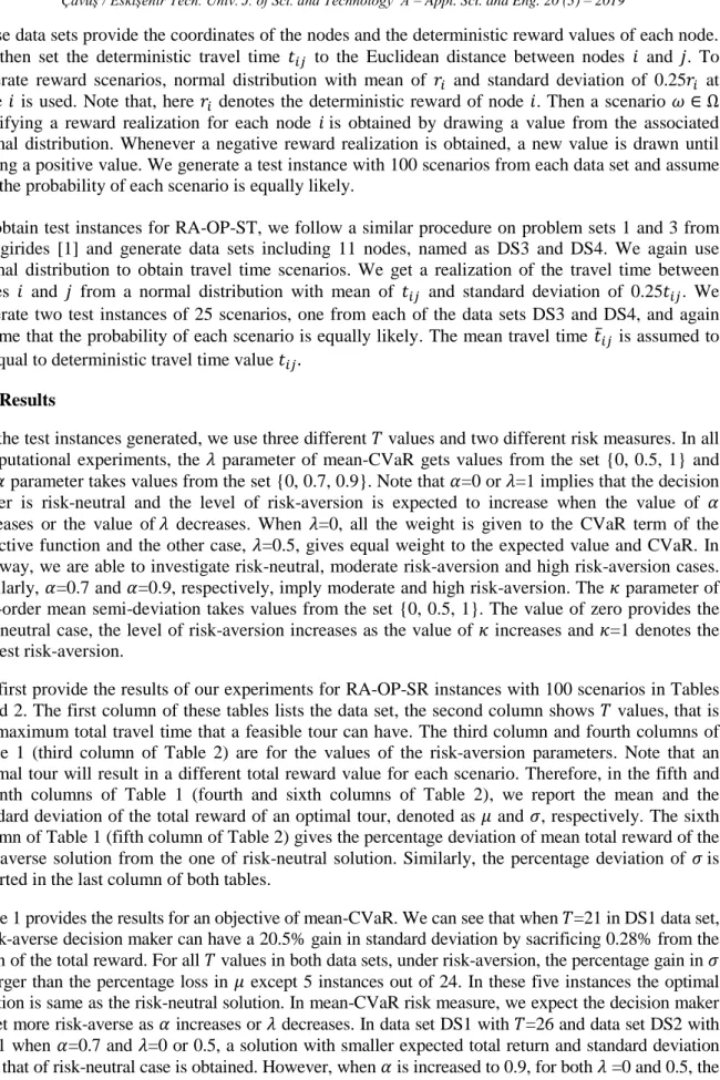
We first provide the results of our experiments for RA-OP-SR instances with 100 scenarios in Tables 1 and 2. The first column of these tables lists the data set, the second column shows 𝑇 values, that is the maximum total travel time that a feasible tour can have. The third column and fourth columns of Table 1 (third column of Table 2) are for the values of the risk-aversion parameters. Note that an optimal tour will result in a different total reward value for each scenario. Therefore, in the fifth and seventh columns of Table 1 (fourth and sixth columns of Table 2), we report the mean and the
standard deviation of the total reward of an optimal tour, denoted as 𝜇 and 𝜎, respectively. The sixth
column of Table 1 (fifth column of Table 2) gives the percentage deviation of mean total reward of the
risk-averse solution from the one of risk-neutral solution. Similarly, the percentage deviation of 𝜎 is
reported in the last column of both tables.
Table 1 provides the results for an objective of mean-CVaR. We can see that when 𝑇=21 in DS1 data set, a risk-averse decision maker can have a 20.5% gain in standard deviation by sacrificing 0.28% from the mean of the total reward. For all 𝑇 values in both data sets, under risk-aversion, the percentage gain in 𝜎
is larger than the percentage loss in 𝜇 except 5 instances out of 24. In these five instances the optimal
solution is same as the risk-neutral solution. In mean-CVaR risk measure, we expect the decision maker to get more risk-averse as 𝛼 increases or 𝜆 decreases. In data set DS1 with 𝑇=26 and data set DS2 with 𝑇=31 when 𝛼=0.7 and 𝜆=0 or 0.5, a solution with smaller expected total return and standard deviation than that of risk-neutral case is obtained. However, when 𝛼 is increased to 0.9, for both 𝜆 =0 and 0.5, the optimal solution is same as the one in risk-neutral case. Such behavior of mean-CVaR at high 𝛼 values is reported in some other studies in the literature, see for instance [26].
Table 1. The results of the problem RA-OP-SR under mean-CvaR Data Set 𝝀 Total Reward 𝑻 𝜶 𝝁 Deviation of 𝝁 (%) 𝝈 Deviation of 𝝈 (%) DS1 0 1 143.3 - 17.1 - 21 0.7 0.7 0 0.5 142.8 142.9 -0.35 -0.28 14.0 13.6 -18.1 -20.5 0.9 0.9 0 0.5 142.9 142.9 -0.28 -0.28 13.6 13.6 -20.5 -20.5 0 1 167.4 - 17.8 - 23 0.7 0.7 0 0.5 166.8 166.8 -0.36 -0.36 14.8 14.8 -16.9 -16.9 0.9 0.9 0 0.5 166.8 166.8 -0.36 -0.36 14.8 14.8 -16.9 -16.9 0 1 208.7 - 19.4 - 26 0.7 0.7 0 0.5 208.6 208.6 -0.05 -0.05 19.3 19.3 -0.5 -0.5 0.9 0.9 0 0.5 208.7 208.7 0 0 19.4 19.4 0 0 DS2 0 1 175.3 - 16.7 - 25 0.7 0.7 0 0.5 174.5 174.5 -0.46 -0.46 15.2 15.2 -9.0 -9.0 0.9 0.9 0 0.5 174.3 174.5 -0.57 -0.46 14.6 15.2 -12.6 -9.0 0 1 248.2 - 19.8 - 31 0.7 0.7 0 0.5 247.7 247.7 -0.20 -0.20 18.9 18.9 -4.5 -4.5 0.9 0.9 0 0.5 248.2 248.2 0 0 19.8 19.8 0 0 0 1 301.9 - 22.4 - 36 0.7 0.7 0 0.5 301.6 301.9 -0.10 0 21.8 22.4 -2.7 0 0.9 0.9 0 0.5 301.6 301.6 -0.10 -0.10 21.8 21.8 -2.7 -2.7
Recall from Section 2, given a random cost 𝑋, CVaR𝛼(𝑋) can be interpreted as the conditional
expectation of 𝑋 values exceeding VaR𝛼(𝑋), where VaR𝛼(𝑋) is 𝛼-quantile of the distribution of 𝑋. In
other words, CVaR𝛼 considers the loss values falling into the tail exceeding 𝛼-quantile. We will call
this tail as 𝛼-upper tail for the rest of the paper. Even the standard deviation of a distribution is large; it might be the case that the dispersion of the 𝛼-upper tail is small. In such cases, mean-CVaR may prefer a cost distribution with high standard deviation to a cost distribution with less standard deviation.
To explain more specifically, we focus on data set DS1 with 𝑇=26. In order to make the explanation
easier, we take λ=0, because in this case, the objective reduces to minimize CVaR value of negative
total reward.
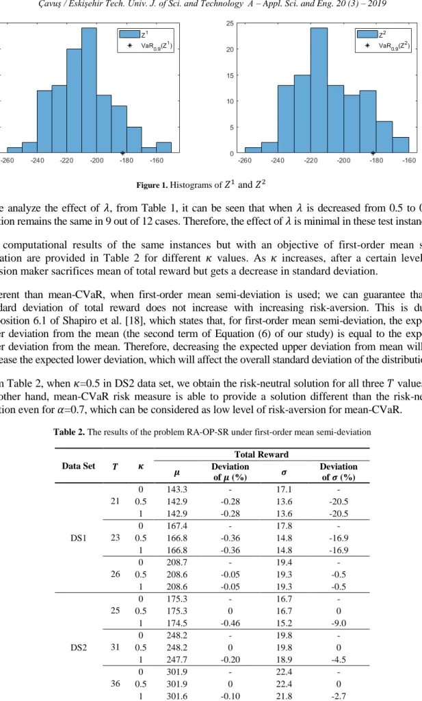
Let 𝑍𝜔1 and 𝑍𝜔2 denote negative of optimal total reward under scenario 𝜔 ∈ Ω when 𝛼=0.7 and 𝛼=0.9,
respectively. Also let 𝑍𝑖 be a discrete random variable for which 𝑍𝑖(𝜔) = 𝑍𝜔𝑖 with probability 1/100
for 𝑖=1,2. We provide the histograms and VaR0.9 values of 𝑍1 and 𝑍2 in Figure 1. It can be seen that
even VaR0.9(𝑍1) and VaR0.9(𝑍2) are close to each other, the 𝛼-upper tail of 𝑍1 is fatter than the
𝛼-upper tail of 𝑍2. Therefore, CVaR0.9(𝑍1) > CVaR0.9(𝑍2) and 𝑍2 is preferred to 𝑍1 at significance level
𝛼 = 0.9. This means that, when risk measure mean-CVaR is used, focusing on tails of random cost distribution exceeding different quantiles, we may have solutions with different behavior.
Figure 1. Histograms of 𝑍1 and 𝑍2
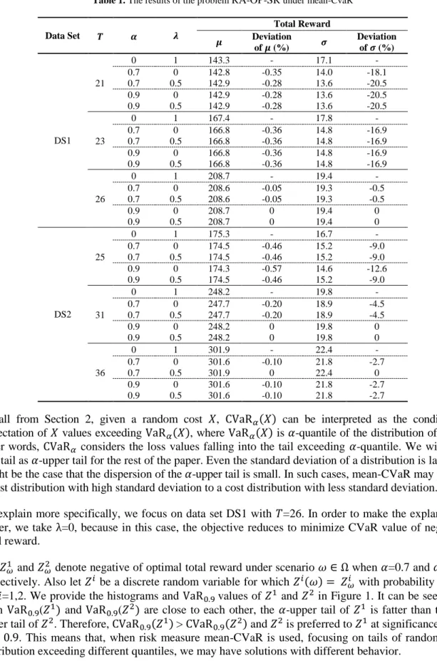
If we analyze the effect of 𝜆, from Table 1, it can be seen that when 𝜆 is decreased from 0.5 to 0, the
solution remains the same in 9 out of 12 cases. Therefore, the effect of 𝜆 is minimal in these test instances. The computational results of the same instances but with an objective of first-order mean
semi-deviation are provided in Table 2 for different 𝜅 values. As 𝜅 increases, after a certain level, the
decision maker sacrifices mean of total reward but gets a decrease in standard deviation.
Different than mean-CVaR, when first-order mean semi-deviation is used; we can guarantee that the standard deviation of total reward does not increase with increasing risk-aversion. This is due to Proposition 6.1 of Shapiro et al. [18], which states that, for first-order mean semi-deviation, the expected upper deviation from the mean (the second term of Equation (6) of our study) is equal to the expected lower deviation from the mean. Therefore, decreasing the expected upper deviation from mean will also decrease the expected lower deviation, which will affect the overall standard deviation of the distribution. From Table 2, when 𝜅=0.5 in DS2 data set, we obtain the risk-neutral solution for all three 𝑇 values. On the other hand, mean-CVaR risk measure is able to provide a solution different than the risk-neutral solution even for 𝛼=0.7, which can be considered as low level of risk-aversion for mean-CVaR.
Table 2. The results of the problem RA-OP-SR under first-order mean semi-deviation
Data Set 𝜿 Total Reward 𝑻 𝝁 Deviation of 𝝁 (%) 𝝈 Deviation of 𝝈 (%) DS1 0 143.3 - 17.1 - 21 0.5 142.9 -0.28 13.6 -20.5 1 142.9 -0.28 13.6 -20.5 0 167.4 - 17.8 - 23 0.5 166.8 -0.36 14.8 -16.9 1 166.8 -0.36 14.8 -16.9 0 208.7 - 19.4 - 26 0.5 208.6 -0.05 19.3 -0.5 1 208.6 -0.05 19.3 -0.5 DS2 0 175.3 - 16.7 - 25 0.5 175.3 0 16.7 0 1 174.5 -0.46 15.2 -9.0 0 248.2 - 19.8 - 31 0.5 248.2 0 19.8 0 1 247.7 -0.20 18.9 -4.5 0 301.9 - 22.4 - 36 0.5 301.9 0 22.4 0 1 301.6 -0.10 21.8 -2.7
In most of RA-OP-SR instances, an optimal tour of a risk-averse decision maker is rather different than an optimal tour of a risk-neutral decision maker. We illustrate this in Figure 2 which includes the optimal tours of risk-neutral and risk-averse decision makers for the data set DS1 with 𝑇=21.
(a)
(b)
Figure 2. Optimal tour of data set DS1 with 𝑇=21 under first-order mean semi-deviation. (a) Risk-neutral solution (𝜅=0); (b) Risk-averse solution (𝜅=0.5 or 𝜅=1).
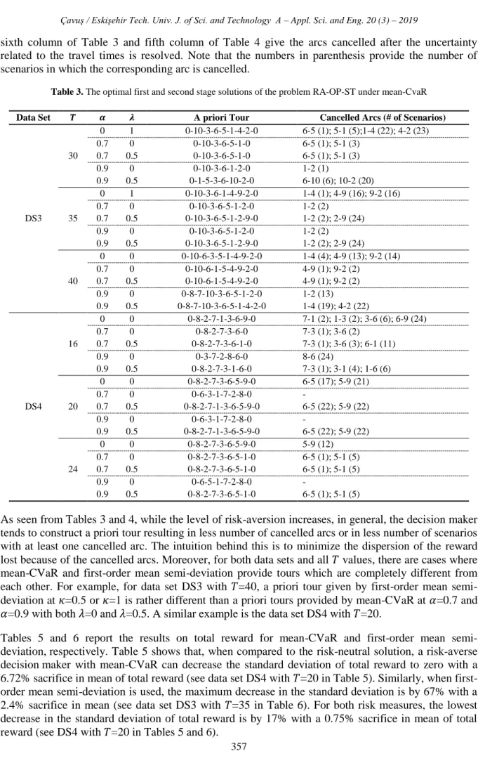
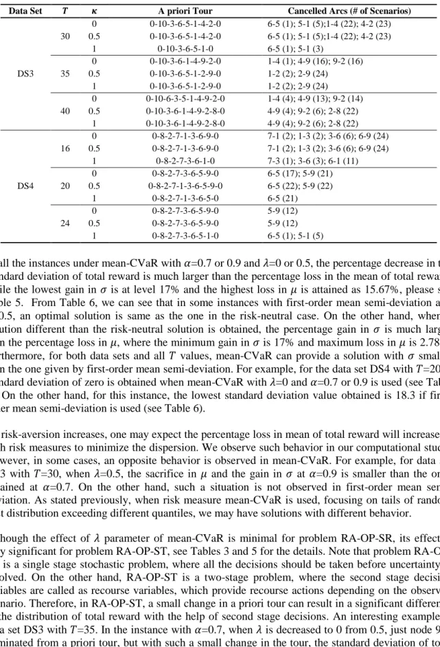
For the case of stochastic travel time (problem RA-OP-ST), test instances with 25 scenarios are generated. Computational results for the constructed tours under mean-CVaR and first-order mean semi-deviation are reported in Tables 3 and 4, respectively. Tables 5 and 6 present the results on the total reward for both risk measures. The first four columns of Table 3 and the first three columns of Table 4 are for the data set, maximum travel time and risk parameters. The fifth column of Table 3 and fourth column of Table 4 provide an optimal a priori tour, where node 0 denotes the depot node. The
sixth column of Table 3 and fifth column of Table 4 give the arcs cancelled after the uncertainty related to the travel times is resolved. Note that the numbers in parenthesis provide the number of scenarios in which the corresponding arc is cancelled.
Table 3. The optimal first and second stage solutions of the problem RA-OP-ST under mean-CvaR Data Set 𝑻 𝜶 𝝀 A priori Tour Cancelled Arcs (# of Scenarios)
DS3 30 0 1 0-10-3-6-5-1-4-2-0 6-5 (1); 5-1 (5);1-4 (22); 4-2 (23) 0.7 0.7 0 0.5 0-10-3-6-5-1-0 0-10-3-6-5-1-0 6-5 (1); 5-1 (3) 6-5 (1); 5-1 (3) 0.9 0.9 0 0.5 0-10-3-6-1-2-0 0-1-5-3-6-10-2-0 1-2 (1) 6-10 (6); 10-2 (20) 35 0 1 0-10-3-6-1-4-9-2-0 1-4 (1); 4-9 (16); 9-2 (16) 0.7 0.7 0 0.5 0-10-3-6-5-1-2-0 0-10-3-6-5-1-2-9-0 1-2 (2) 1-2 (2); 2-9 (24) 0.9 0.9 0 0.5 0-10-3-6-5-1-2-0 0-10-3-6-5-1-2-9-0 1-2 (2) 1-2 (2); 2-9 (24) 40 0 0 0-10-6-3-5-1-4-9-2-0 1-4 (4); 4-9 (13); 9-2 (14) 0.7 0.7 0 0.5 0-10-6-1-5-4-9-2-0 0-10-6-1-5-4-9-2-0 4-9 (1); 9-2 (2) 4-9 (1); 9-2 (2) 0.9 0.9 0 0.5 0-8-7-10-3-6-5-1-2-0 0-8-7-10-3-6-5-1-4-2-0 1-2 (13) 1-4 (19); 4-2 (22) DS4 16 0 0 0-8-2-7-1-3-6-9-0 7-1 (2); 1-3 (2); 3-6 (6); 6-9 (24) 0.7 0.7 0 0.5 0-8-2-7-3-6-0 0-8-2-7-3-6-1-0 7-3 (1); 3-6 (2) 7-3 (1); 3-6 (3); 6-1 (11) 0.9 0.9 0 0.5 0-3-7-2-8-6-0 0-8-2-7-3-1-6-0 8-6 (24) 7-3 (1); 3-1 (4); 1-6 (6) 20 0 0 0-8-2-7-3-6-5-9-0 6-5 (17); 5-9 (21) 0.7 0.7 0 0.5 0-6-3-1-7-2-8-0 0-8-2-7-1-3-6-5-9-0 - 6-5 (22); 5-9 (22) 0.9 0.9 0 0.5 0-6-3-1-7-2-8-0 0-8-2-7-1-3-6-5-9-0 - 6-5 (22); 5-9 (22) 24 0 0 0-8-2-7-3-6-5-9-0 5-9 (12) 0.7 0.7 0 0.5 0-8-2-7-3-6-5-1-0 0-8-2-7-3-6-5-1-0 6-5 (1); 5-1 (5) 6-5 (1); 5-1 (5) 0.9 0.9 0 0.5 0-6-5-1-7-2-8-0 0-8-2-7-3-6-5-1-0 - 6-5 (1); 5-1 (5)
As seen from Tables 3 and 4, while the level of risk-aversion increases, in general, the decision maker tends to construct a priori tour resulting in less number of cancelled arcs or in less number of scenarios with at least one cancelled arc. The intuition behind this is to minimize the dispersion of the reward lost because of the cancelled arcs. Moreover, for both data sets and all 𝑇 values, there are cases where mean-CVaR and first-order mean semi-deviation provide tours which are completely different from
each other. For example, for data set DS3 with 𝑇=40, a priori tour given by first-order mean
semi-deviation at 𝜅=0.5 or 𝜅=1 is rather different than a priori tours provided by mean-CVaR at 𝛼=0.7 and 𝛼=0.9 with both 𝜆=0 and 𝜆=0.5. A similar example is the data set DS4 with 𝑇=20.
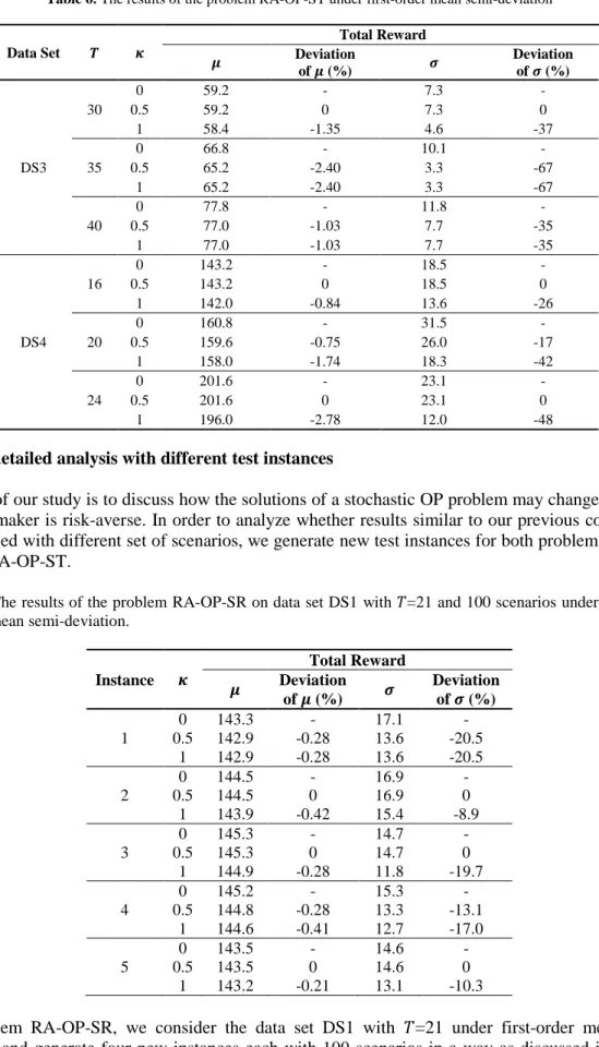
Tables 5 and 6 report the results on total reward for mean-CVaR and first-order mean semi-deviation, respectively. Table 5 shows that, when compared to the risk-neutral solution, a risk-averse decision maker with mean-CVaR can decrease the standard deviation of total reward to zero with a 6.72% sacrifice in mean of total reward (see data set DS4 with 𝑇=20 in Table 5). Similarly, when first-order mean semi-deviation is used, the maximum decrease in the standard deviation is by 67% with a 2.4% sacrifice in mean (see data set DS3 with 𝑇=35 in Table 6). For both risk measures, the lowest decrease in the standard deviation of total reward is by 17% with a 0.75% sacrifice in mean of total reward (see DS4 with 𝑇=20 in Tables 5 and 6).
Table 4. The optimal first and second stage solutions of the problem RA-OP-ST under first-order mean semi-deviation Data Set 𝑻 𝜿 A priori Tour Cancelled Arcs (# of Scenarios)
DS3 30 0 0-10-3-6-5-1-4-2-0 6-5 (1); 5-1 (5);1-4 (22); 4-2 (23) 0.5 0-10-3-6-5-1-4-2-0 6-5 (1); 5-1 (5);1-4 (22); 4-2 (23) 1 0-10-3-6-5-1-0 6-5 (1); 5-1 (3) 35 0 0-10-3-6-1-4-9-2-0 1-4 (1); 4-9 (16); 9-2 (16) 0.5 0-10-3-6-5-1-2-9-0 1-2 (2); 2-9 (24) 1 0-10-3-6-5-1-2-9-0 1-2 (2); 2-9 (24) 40 0 0-10-6-3-5-1-4-9-2-0 1-4 (4); 4-9 (13); 9-2 (14) 0.5 0-10-3-6-1-4-9-2-8-0 4-9 (4); 9-2 (6); 2-8 (22) 1 0-10-3-6-1-4-9-2-8-0 4-9 (4); 9-2 (6); 2-8 (22) DS4 16 0 0-8-2-7-1-3-6-9-0 7-1 (2); 1-3 (2); 3-6 (6); 6-9 (24) 0.5 0-8-2-7-1-3-6-9-0 7-1 (2); 1-3 (2); 3-6 (6); 6-9 (24) 1 0-8-2-7-3-6-1-0 7-3 (1); 3-6 (3); 6-1 (11) 20 0 0-8-2-7-3-6-5-9-0 6-5 (17); 5-9 (21) 0.5 0-8-2-7-1-3-6-5-9-0 6-5 (22); 5-9 (22) 1 0-8-2-7-1-3-6-5-0 6-5 (21) 24 0 0-8-2-7-3-6-5-9-0 5-9 (12) 0.5 0-8-2-7-3-6-5-9-0 5-9 (12) 1 0-8-2-7-3-6-5-1-0 6-5 (1); 5-1 (5)
In all the instances under mean-CVaR with 𝛼=0.7 or 0.9 and 𝜆=0 or 0.5, the percentage decrease in the standard deviation of total reward is much larger than the percentage loss in the mean of total reward,
while the lowest gain in 𝜎 is at level 17% and the highest loss in 𝜇 is attained as 15.67%, please see
Table 5. From Table 6, we can see that in some instances with first-order mean semi-deviation and 𝜅=0.5, an optimal solution is same as the one in the risk-neutral case. On the other hand, when a
solution different than the risk-neutral solution is obtained, the percentage gain in 𝜎 is much larger
than the percentage loss in 𝜇, where the minimum gain in 𝜎 is 17% and maximum loss in 𝜇 is 2.78%.
Furthermore, for both data sets and all 𝑇 values, mean-CVaR can provide a solution with 𝜎 smaller
than the one given by first-order mean semi-deviation. For example, for the data set DS4 with 𝑇=20, a standard deviation of zero is obtained when mean-CVaR with 𝜆=0 and 𝛼=0.7 or 0.9 is used (see Table 5). On the other hand, for this instance, the lowest standard deviation value obtained is 18.3 if first-order mean semi-deviation is used (see Table 6).
As risk-aversion increases, one may expect the percentage loss in mean of total reward will increase in both risk measures to minimize the dispersion. We observe such behavior in our computational study. However, in some cases, an opposite behavior is observed in mean-CVaR. For example, for data set
DS3 with 𝑇=30, when 𝜆=0.5, the sacrifice in 𝜇 and the gain in 𝜎 at 𝛼=0.9 is smaller than the ones
obtained at 𝛼=0.7. On the other hand, such a situation is not observed in first-order mean
semi-deviation. As stated previously, when risk measure mean-CVaR is used, focusing on tails of random cost distribution exceeding different quantiles, we may have solutions with different behavior.
Although the effect of 𝜆 parameter of mean-CVaR is minimal for problem RA-OP-SR, its effect is
very significant for problem ST, see Tables 3 and 5 for the details. Note that problem RA-OP-SR is a single stage stochastic problem, where all the decisions should be taken before uncertainty is resolved. On the other hand, RA-OP-ST is a two-stage problem, where the second stage decision variables are called as recourse variables, which provide recourse actions depending on the observed scenario. Therefore, in RA-OP-ST, a small change in a priori tour can result in a significant difference in the distribution of total reward with the help of second stage decisions. An interesting example is data set DS3 with 𝑇=35. In the instance with 𝛼=0.7, when 𝜆 is decreased to 0 from 0.5, just node 9 is eliminated from a priori tour, but with such a small change in the tour, the standard deviation of total
reward decreases to 1.4 from 3.3. When 𝜆=0.5, arc (2,9) is cancelled in 24 scenarios out of 25. Therefore, eliminating node 9 from the tour results in a significant decrease in the standard deviation.
Similarly, in data set DS4 with 𝑇=20 and 𝛼=0.9, when 𝜆 is decreased to 0 from 0.5, the standard
deviation decreases to zero from 26 by eliminating nodes 5 and 9 from a priori tour.
Table 5. The results of the problem RA-OP-ST under mean-CvaR
Data Set 𝑻 𝝀 Total Reward 𝜶 𝝁 Deviation of 𝝁 (%) 𝝈 Deviation of 𝝈 (%) DS3 30 0 1 59.2 - 7.3 - 0.7 0.7 0 0.5 58.4 58.4 -1.35 -1.35 4.6 4.6 -37 -37 0.9 0.9 0 0.5 54.8 58.6 -7.43 -1.01 1.0 5.0 -86 -32 35 0 1 66.8 - 10.1 - 0.7 0.7 0 0.5 64.6 65.2 -3.29 -2.40 1.4 3.3 -86 -67 0.9 0.9 0 0.5 64.6 65.2 -3.29 -2.40 1.4 3.3 -86 -67 40 0 1 77.8 - 11.8 - 0.7 0.7 0 0.5 74.0 74.0 -4.88 -4.88 4.0 4.0 -66 -66 0.9 0.9 0 0.5 72.4 73.0 -6.94 -6.17 2.5 5.5 -78 -53 DS4 16 0 1 143.2 - 18.5 - 0.7 0.7 0 0.5 137.2 142.0 -4.19 -0.70 10.4 13.6 -44 -26 0.9 0.9 0 0.5 120.8 142.4 -0.84 -0.56 3.9 15.0 -79 -19 20 0 1 160.8 - 31.5 - 0.7 0.7 0 0.5 150.0 159.6 -6.72 -0.75 0 26.0 -100 -17 0.9 0.9 0 0.5 150.0 159.6 -6.72 -0.75 0 26.0 -100 -17 24 0 1 201.6 - 23.1 - 0.7 0.7 0 0.5 196.0 196.0 -2.78 -2.78 12.0 12.0 -48 -48 0.9 0.9 0 0.5 170.0 196.0 -15.67 -2.78 0 12.0 -100 -48
From Tables 3 and 5, it can be seen that, in 9 out of 12 cases, a different solution is obtained if 𝜆 is
decreased to 0 from 0.5. When 𝜆=0, the objective function gives all the weight to CVaR and
completely ignores the mean of total reward. In this case, however, a significant sacrifice in mean may occur as in data set DS4 with 𝑇=24 and 𝛼=0.9, which may be undesirable by the decision maker.
Table 6. The results of the problem RA-OP-ST under first-order mean semi-deviation Data Set 𝑻 𝜿 Total Reward 𝝁 Deviation of 𝝁 (%) 𝝈 Deviation of 𝝈 (%) DS3 30 0 59.2 - 7.3 - 0.5 59.2 0 7.3 0 1 58.4 -1.35 4.6 -37 35 0 66.8 - 10.1 - 0.5 65.2 -2.40 3.3 -67 1 65.2 -2.40 3.3 -67 40 0 77.8 - 11.8 - 0.5 77.0 -1.03 7.7 -35 1 77.0 -1.03 7.7 -35 DS4 16 0 143.2 - 18.5 - 0.5 143.2 0 18.5 0 1 142.0 -0.84 13.6 -26 20 0 160.8 - 31.5 - 0.5 159.6 -0.75 26.0 -17 1 158.0 -1.74 18.3 -42 24 0 201.6 - 23.1 - 0.5 201.6 0 23.1 0 1 196.0 -2.78 12.0 -48
4.2.1. A detailed analysis with different test instances
The aim of our study is to discuss how the solutions of a stochastic OP problem may change when the decision maker is risk-averse. In order to analyze whether results similar to our previous conclusions are obtained with different set of scenarios, we generate new test instances for both problems RA-OP-SR and RA-OP-ST.
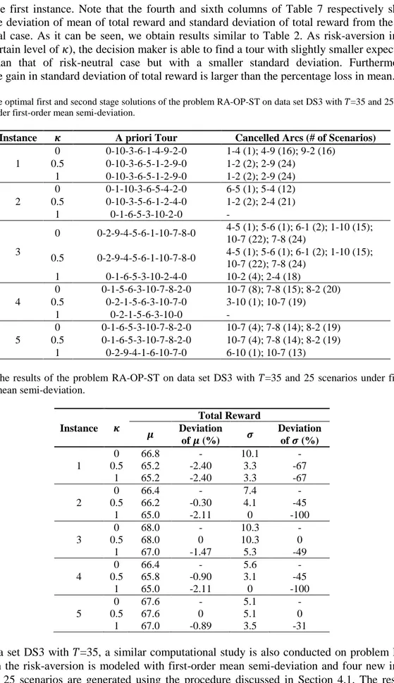
Table 7. The results of the problem RA-OP-SR on data set DS1 with 𝑇=21 and 100 scenarios under first-order mean semi-deviation. 𝜿 Total Reward Instance 𝝁 Deviation of 𝝁 (%) 𝝈 Deviation of 𝝈 (%) 0 143.3 - 17.1 - 1 0.5 142.9 -0.28 13.6 -20.5 1 142.9 -0.28 13.6 -20.5 0 144.5 - 16.9 - 2 0.5 144.5 0 16.9 0 1 143.9 -0.42 15.4 -8.9 0 145.3 - 14.7 - 3 0.5 145.3 0 14.7 0 1 144.9 -0.28 11.8 -19.7 0 145.2 - 15.3 - 4 0.5 144.8 -0.28 13.3 -13.1 1 144.6 -0.41 12.7 -17.0 0 143.5 - 14.6 - 5 0.5 143.5 0 14.6 0 1 143.2 -0.21 13.1 -10.3
For problem RA-OP-SR, we consider the data set DS1 with 𝑇=21 under first-order mean
semi-deviation and generate four new instances each with 100 scenarios in a way as discussed in Section 4.1. The results of new instances are provided in Table 7. For comparison purpose, the old instance is
kept as the first instance. Note that the fourth and sixth columns of Table 7 respectively show the percentage deviation of mean of total reward and standard deviation of total reward from the ones of risk-neutral case. As it can be seen, we obtain results similar to Table 2. As risk-aversion increases (after a certain level of 𝜅), the decision maker is able to find a tour with slightly smaller expected total reward than that of risk-neutral case but with a smaller standard deviation. Furthermore, the percentage gain in standard deviation of total reward is larger than the percentage loss in mean.
Table 8. The optimal first and second stage solutions of the problem RA-OP-ST on data set DS3 with 𝑇=35 and 25 scenarios under first-order mean semi-deviation.
Instance 𝜿 A priori Tour Cancelled Arcs (# of Scenarios)
1 0 0-10-3-6-1-4-9-2-0 1-4 (1); 4-9 (16); 9-2 (16) 0.5 0-10-3-6-5-1-2-9-0 1-2 (2); 2-9 (24) 1 0-10-3-6-5-1-2-9-0 1-2 (2); 2-9 (24) 2 0 0-1-10-3-6-5-4-2-0 6-5 (1); 5-4 (12) 0.5 0-10-3-5-6-1-2-4-0 1-2 (2); 2-4 (21) 1 0-1-6-5-3-10-2-0 - 3 0 0-2-9-4-5-6-1-10-7-8-0 4-5 (1); 5-6 (1); 6-1 (2); 1-10 (15); 10-7 (22); 7-8 (24) 0.5 0-2-9-4-5-6-1-10-7-8-0 4-5 (1); 5-6 (1); 6-1 (2); 1-10 (15); 10-7 (22); 7-8 (24) 1 0-1-6-5-3-10-2-4-0 10-2 (4); 2-4 (18) 4 0 0-1-5-6-3-10-7-8-2-0 10-7 (8); 7-8 (15); 8-2 (20) 0.5 0-2-1-5-6-3-10-7-0 3-10 (1); 10-7 (19) 1 0-2-1-5-6-3-10-0 - 5 0 0-1-6-5-3-10-7-8-2-0 10-7 (4); 7-8 (14); 8-2 (19) 0.5 0-1-6-5-3-10-7-8-2-0 10-7 (4); 7-8 (14); 8-2 (19) 1 0-2-9-4-1-6-10-7-0 6-10 (1); 10-7 (13)
Table 9. The results of the problem RA-OP-ST on data set DS3 with 𝑇=35 and 25 scenarios under first-order mean semi-deviation. 𝜿 Total Reward Instance 𝝁 Deviation of 𝝁 (%) 𝝈 Deviation of 𝝈 (%) 0 66.8 - 10.1 - 1 0.5 65.2 -2.40 3.3 -67 1 65.2 -2.40 3.3 -67 0 66.4 - 7.4 - 2 0.5 66.2 -0.30 4.1 -45 1 65.0 -2.11 0 -100 0 68.0 - 10.3 - 3 0.5 68.0 0 10.3 0 1 67.0 -1.47 5.3 -49 0 66.4 - 5.6 - 4 0.5 65.8 -0.90 3.1 -45 1 65.0 -2.11 0 -100 0 67.6 - 5.1 - 5 0.5 67.6 0 5.1 0 1 67.0 -0.89 3.5 -31
Using data set DS3 with 𝑇=35, a similar computational study is also conducted on problem RA-OP-ST. Again the risk-aversion is modeled with first-order mean semi-deviation and four new instances each with 25 scenarios are generated using the procedure discussed in Section 4.1. The results are presented in Tables 8 and 9. Similar to our previous results, as risk-aversion increases, the decision
maker tends to construct a priori tour resulting in less number of cancelled arcs or in less number of scenarios with at least one cancelled arc. Also, as expected, the percentage gain in the standard deviation of total reward is larger than the percentage loss in mean.
With these new computations, it is possible to conclude that our results on risk-averse decisions do not change with different instances of both problems.
5. CONCLUSION
In this study, we consider two different stochastic orienteering problems: one with random rewards and the other one with random travel times. For both problems, we propose a risk-averse stochastic programming formulation with an objective of coherent measures of risk. The numerical results conducted on different problem instances show that, for each orienteering problem, a risk-averse solution might be significantly different than the risk-neutral solution in terms of the constructed tour. Furthermore, the risk-averse solutions may provide a significant decrease in the standard deviation of total reward without sacrificing much from the expected total reward.
Since the formulation suggested for OP with stochastic travel times is a two-stage stochastic model, it is much more difficult to solve than the static stochastic model suggested for OP with random rewards. Furthermore, the risk-averse objective function brings additional complexity in solving both models. As a future research direction, a solution methodology can be proposed for the problem RA-OP-ST in order to solve instances with large number of scenarios on larger networks.
REFERENCES
[1] Tsiligirides T. Heuristic Methods Applied to Orienteering. The Journal of the Operational Research Society 1984; 35(9): 797-809.
[2] Golden BL, Levy L, Vohra R. The orienteering problem. Naval Research Logistics 1987; 34(3): 307-318.
[3] Vansteenwegen P, Souffriau W, Van Oudheusden D. The orienteering problem: A survey. European Journal of Operational Research 2011; 209 (1): 1–10.
[4] Gunawan A, Lau HC, Vansteenwegen P. Orienteering problem: A survey of recent variants, solution approaches and applications. European Journal of Operational Research 2016; 255(2): 315-332.
[5] Teng SY, Ong HL, Huang HC. An integer L-shaped algorithm for the time-constrained traveling salesman problem with stochastic travel times and service times. Asia-Pacific Journal of Operational Research 2004; 21: 241–257.
[6] Campbell AM, Gendreau M, Thomas BW. The orienteering problem with stochastic travel and service times. Annals of Operations Research 2011; 186: 61–81.
[7] Tang H, Miller-Hooks E. Algorithms for a stochastic selective travelling salesperson problem. Journal of the Operational Research Society 2005; 56(4): 439–452.
[8] Ilhan T, Iravani SM, Daskin MS. The orienteering problem with stochastic profits. IIE Transactions 2008; 40: 406–421.
[9] Evers L, Glorie K, Van Der Ster S, Barros AI, Monsuur H. A two-stage approach to the orienteering problem with stochastic weights. Computers & Operations Research 2014; 43: 248-260.
[10] Shang K, Chan FT, Karungaru S, Terada K, Feng Z, Ke L. Two-stage robust optimization for orienteering problem with stochastic weights. 2016; arXiv preprint arXiv:1701.00090.
[11] Varakantham P, Kumar A. Optimization approaches for solving chance constrained stochastic orienteering problems. In: International Conference on Algorithmic Decision Theory (ADT); 13-15 November 2013; Bruxelles, Belgium. Springer, Berlin, Heidelberg. pp. 387-398.
[12] Dolinskaya I, Shi ZE, Smilowitz K. Adaptive orienteering problem with stochastic travel times. Transportation Research Part E: Logistics and Transportation Review 2018; 109: 1-19. [13] Hoong CL, William Y, Pradeep V, Duc TN, Huaxing C. Dynamic stochastic orienteering
problems for risk-aware applications. In: Proceedings of the Conference on Uncertainty in Artificial Intelligence (UAI); 15-17 August 2012; Catalina Island, United States. Oregon, USA: AUAI. pp. 448–458.
[14] Varakantham P, Kumar A, Lau HC, Yeoh W. Risk-sensitive stochastic orienteering problems for trip optimization in urban environments. ACM Transactions on Intelligent Systems and Technology (TIST) 2018; 9(3): 24.
[15] Verbeeck C, Vansteenwegen P, Aghezzaf EH. Solving the stochastic time-dependent orienteering problem with time windows. European Journal of Operational Research 2016; 255(3): 699-718. [16] Zhang S, Ohlmann JW, Thomas BW. A priori orienteering with time windows and stochastic
wait times at customers. European Journal of Operational Research 2014; 239(1): 70-79.
[17] Zhang S, Ohlmann JW, Thomas BW. Dynamic orienteering on a network of queues. Transportation Science 2018; 52(3): 691-706.
[18] Shapiro A, Dentcheva D, Ruszczyński A. Lectures on stochastic programming: modeling and theory. Society for Industrial and Applied Mathematics, 2009.
[19] Artzner P, Delbaen F, Eber JM, Heath D. Coherent measures of risk. Mathematical finance 1999; 9(3): 203-228.
[20] Ruszczynski A, Shapiro A. Optimization of convex risk functions. Mathematics of operations research 2006; 31(3): 433–452 .
[21] Ruszczynski A, Shapiro A. Optimization of Risk Measures. In: Calafiore G, Dabbene F, editors. Probabilistic and Randomized Methods for Design under Uncertainty. Springer, London, 2006. pp. 119-157.
[22] Rockafellar RT, Uryasev SP. Optimization of conditional value-at-risk. Journal of Risk 2000; 2: 21-42.
[23] Rockafellar RT, Uryasev SP. Conditional value-at-risk for general loss distributions. Journal of Banking and Finance 2002; 26: 1443-1471.
[24] Rockafellar RT. Coherent approaches to risk in optimization under uncertainty. INFORMS Tutorials in Operations Research. Institute for Operations Research and the Management Sciences, Hanover, MD, 2007. pp. 38–61.
[25] Chao I, Golden B, Wasil E. Theory and Methodology - A fast and effective heuristic for the Orienteering Problem. European Journal of Operational Research 1996; 88: 475-489.
[26] Noyan N. Risk-averse two-stage stochastic programming with an application to disaster management. Computers and Operations Research 2012; 39(3): 541 – 559.