ϋί',·0 *··?Γ'»τ‘-Wí Ь- ii’whiM ,*·* filw·· f# ¥ ·- »MÎ V ' 'i'. '•'»^ ¿ ^ ‘Wiûir· лы ·»¿ i _ uí ΐ L Ы *·> “< ív u' ·.'· Ä* »'«Lîİi, '
*iiw· V· ■••b v·*.·^'
L J’’ ·“■'’■ i
гг^и^--MAXIMUM LIKELIHOOD ESTIMATION OF
PARAMETERS OF SUPERIMPOSED SIGNALS BY
USING TREE-STRUCTURED EM ALGORITHM
A THESIS
SUBMITTED TO THE DEPARTMENT OF ELECTRICAL AND ELECTRONICS ENGINEERING
AND THE INSTITUTE OF ENGINEERING AND SCIENCES OF BILKENT UNIVERSITY
IN PARTIAL FULFILLMENT OF THE REQUIREMENTS FOR THE DEGREE OF
MASTER OF SCIENCE
By
„..Sait Kubilay Pakin
'
...-νβ 3 ? î -rV QO q O
I certify that I have read this thesis and that in my opinion it is fully adequate,
in scope and in quality, as a thesis for the degree of Master of Science.
Asst. Prof. Dr. Orhan Ankan (Supervisor)
I certify that I have read this thesis and that in my opinion it is fully adequate,
in scope and in quality, as a thesis for the degree of Master of Science.
Prof. Dr. M. Erol Sezer
I certify that I have read this thesis and that in my opinion it is fully adequate,
in scope and in quality, as a thesis for the degree of Master of Science.
Asst. Prof. Dr. Billur Barshan
Approved for the Institute of Engineering and Sciences:
Prof. Dr. Mehmet
Director of Institute of Engineermg and Sciences
ABSTRACT
M A X I M U M L IK E L IH O O D E S T IM A T IO N O F
P A R A M E T E R S O F S U P E R IM P O S E D S IG N A L S B Y U SIN G T R E E -S T R U C T U R E D E M A L G O R IT H M
Sait Kubilay Pakin
M .S . in Electrical and Electronics Engineering Supervisor: Asst. Prof. Dr. Orhan Arikan
July 1997
As an extension to the conventional EM algorithm, tree-structured EM algo rithm is proposed for the ML estimation of parameters of superimposed signals. For the special case of superimposed signals in Gaussian noise, the IQML al gorithm of Breşler and Macovski [19] is incorporated to the M-step of the EM based algorithms resulting in more efficient and reliable maximization. Based on simulations, it is observed that TSEM converges significantly faster than EM, but it is more sensitive to the initial parameter estimates. Hybrid-EM al gorithm, which performs a few EM iterations prior to the TSEM iterations, is proposed to capture the desired features of both the EM and TSEM algorithms. Based on simulations, it is found that Hybrid-EM algorithm has significantly more robust convergence than both the EM and TSEM algorithms.
Keywords : Maximum Likelihood Estimation, EM Algorithm, Tree-Structured
EM Algorithm, Hybrid-EM Algorithm, Parameter Estimation.
ÖZET
b i r b i r i n e e k l e n m i ş i ş a r e t l e r e A İ T
D E Ğ İŞ K E N L E R İN D A L L I B E Y Ö N T E M İ K U L L A N IL A R A K E N O L A S I K E S T İR İM İ
Sait Kubilay Pakin
Elektrik ve Elektronik Mühendisliği Bölümü Yüksek Lisans Tez Yöneticisi: Yrd. Doç. Dr. Orhan Arıkan
Tem m uz 1997
Birbirine eklenmiş işaretlerin değişkenlerinin en olası kestirimi için, bili nen Beklenti Enbüyûkleme (BE) yöntemini geliştirmek üzere, Dallı Bek lenti Enbûyûkleme (DBE) jüntemi önerilmiştir. Özel bir durum olan Gauss dağilimli gürültü içinde birbirine eklenmiş olan sinüzoidal işaretler için, Breşler ve Maıcovski [19] tarafından önerilmiş olan IQML yöntemi, BE ta banlı yöntemlerin en büyükleme adımında kullanılarak, daha güvenilir ve verimli enbûyûkleme gerçekleştirilmiştir. Benzetimler DBE yönteminin BE jmnteminden daha hızlı yakınsamasına rağmen, değişkenlerin ilk kestirimler- ine daha hassas olduğunu göstermiştir. BE ve DBE yöntemlerinin arzu lanan özelliklerini bir arada toplamak için, DBE yinelemelerinden önce birkaç BE yinelemesi yapan Karma-BE yöntemi önerilmiştir. Benzetimler, Karma- BE yönteminin, BE ve DBE yöntemlerinden daha gürbüz yakınsamaya sahip olduğunu göstermiştir.
Anahtar Kelimeler: Enbüyûk Olabilirlik Kestirimi (En Olası Kestirim), BE
Yöntemi, Dallı BE Yöntemi, Karma-BE Yöntemi, Değişken Kestirimi.
ACKNOWLEDGEMENT
I would like to express my deep gratitude to my supervisor Dr.Orhan Arikan for his supervision, guidance, suggestions and invaluable encouragement through out the development of this thesis. I am also deeply indebted to Dr. M. Erol
Sezer and Dr. Billur Barshan for their reading and commenting on the thesis.
A special note of thanks is due my dear sister Ebru for her continuous support.
And sincere thanks to my dearest Ayşegül for her understanding, patience and love.
TABLE OF CONTENTS
1 Introduction 1
2 Parametric Signal Decomposition by Maximum Likelihood Es
timation 4
3 EM Algorithm and its Application to Superimposed Signal
Model 7
4 Tree-Structured EM Algorithm and its Application to Super
imposed Signal Model 11
5 Parameter Estimation of Superimposed Exponentials in Noise 15
6 Simulations
20
6.1 Simulation Set 1 : Case of Four Exponential Signal Components 20
6.2 Simulation Set 2 : Case of Eight Exponential Signal Components 29
7 Conclusions and Future Work 32
APPEN D IX 36
A Iterative Quadratic Maximum Likelihood (IQML) Algorithm 37 B Cramer-Rao Lower Bound 39
LIST OF FIGURES
4.1 The binary tree structure between complete and incomplete data spaces for the case of number of signals M = 2” +^... 12
4.2 A detail from the binary tree structure... 12
•5.1 The block diagram of one iteration of IQML-EM algorithm. 17
6.1
6.2
6.3
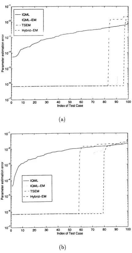
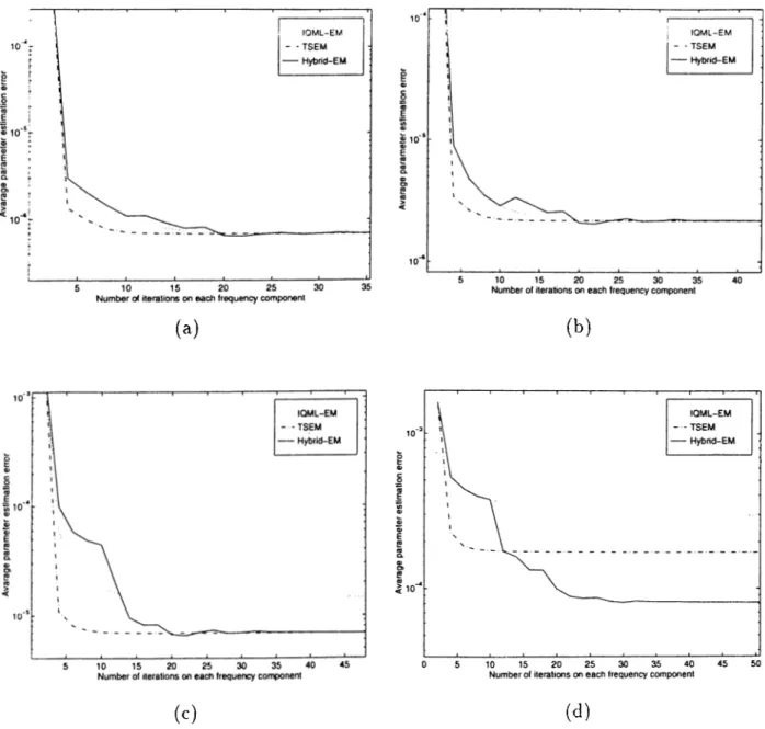
Sorted resulting parameter estimation errors for 100 runs of IQML, IQML-EM, TSEM, and H)'brid-EM algorithms with dif ferent initial estimates determined by Eqn.(6.3). The figures in (a) and (b) correspond to r] = 0.055 and 77 = 0.1, respectively. The tracks o f average parameter estimation error of the IQML- EM, TSEM. and Hybrid-EM algorithms for (a) 5 dB, (b) 0 dB, (c) —5 dB, and (d) —10 dB SNR values. The initial estimates of frequency parameters were = [0.16 0.30 0.54 0.42]^. . .
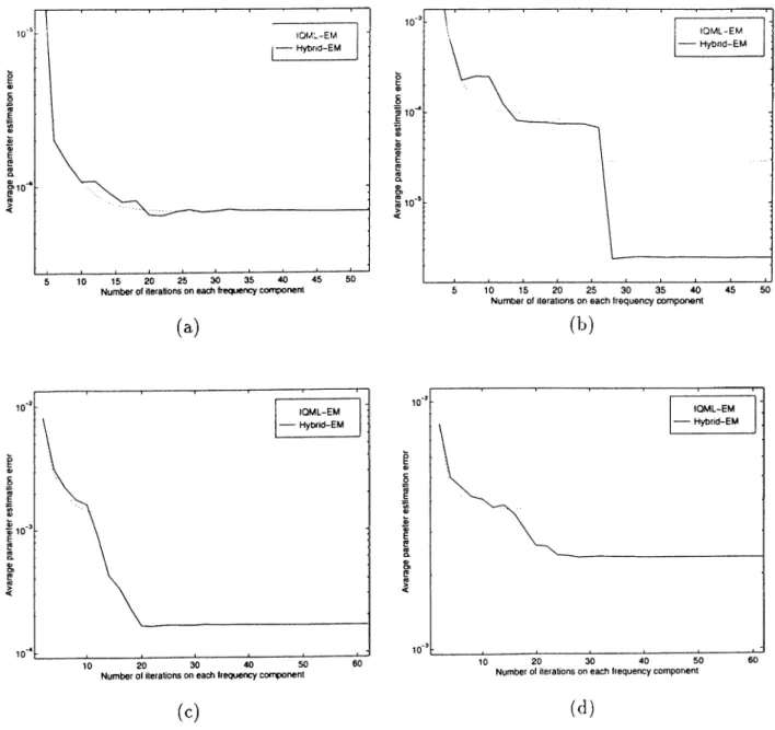
The tracks of average parameter estimation error of EM and Hybrid-EM algorithms for (a) 5 dB, (b) 0 dB, (c) - 5 dB, and (d) —10 dB SNR values. The initial estimates of frequency pa rameters were = [0.13 0.28 0.57 0.44]^...
24
25
26
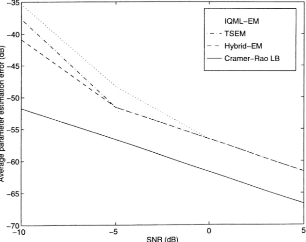
6.4 Frequency parameter estimation errors of IQML-EM, TSEM, and Hj'brid-EM algorithms with Cramer-Rao lower bound. . . . 27
6.5 (a) : Amplitude estimation errors of IQML-EM, TSEM, and Hybrid-EM algorithms with Cramer-Rao lower bound, (b) : The track of average amplitude estimation error of IQML-EM, TSEM, and Hybrid-EM algorithms for 0 dB SNR...
6.6 Tree structured mapping in the case of 8 sig n a ls...
28
29
6.7 The tracks of average parameter estimation error of IQML- EM, TSEM, and Hybrid-EM algorithms for (a) 5 dB, (b) 0 dB, (c) - 5 dB, and (d) - 1 0 dB SNR values. 9° =
[0.23 0.20 0.28 0.37 0.43 0.41 0.54 0.48]^ has been set as the initial parameter estimates... 31
Chapter 1
Introduction
Decomposition of signals into a parametric family of subcomponents have been a requirement of various signal processing applications including array signal processing, time-frequency atomic decompositions, magnetic resonance imag ing and seismic imaging [l]-[5]. In the absence of prior information on the parameters of the signal components, maximum likelihood estimation of the parameters provides the optimal signal decomposition. However, the required multidimensional optimization of the likelihood function over the parameter space is not only computationally very intensive but due to the complicated local minima structure of the likelihood surface, convergence of gradient de scent optimizers to the global maxima is not guaranteed. For these reasons, suboptimal parameter estimation methods are extensivel}' emplo3"ed in prac tice [6]-[8].
Recently, an iterative procedure known as Expectation-Maximization (EM) algorithm which provides the maximum likelihood estimate of the parame ters has stirred up the interest in the applications of maximum likelihood ap proach [3], [9]-[13]. In EM formalism, the available observations forming the incomplete data are obtained via a many-to-one mapping from the complete data space that includes the individual signal components. The EM algorithm iterates between estimating the log-likelihood of complete data using the incom plete data and the current parameter estimates (E-step), and maximizing the
estimated log-likelihood function to obtain the updated parameter estimates (M-step). Under mild regularity conditions, the iterations of the EM algorithm converges to a stationary point of the observed log-likelihood function, where at each iteration the likelihood of the estimated parameters increases [14. 15]. However, as shown in the application to tlie wide-band direction of arrival es timation, straightforward application of EM algorithm is not so successful [16]. Convergence of the EM iterations considerably slows down when the number of estimated parameters increases.
In order to improve the performance of EM algorithm, three extensions have been proposed. In the earliest of these extensions, known as Cascade EM (CEM ), an intermediate complete data specification between the complete and incomplete data of the conventional EM method is used. It was reported that the CEM algorithm has faster convergence and needs less computations per iteration than the EM algorithm [17]. The second extension of the EM algo rithm is the Space Alternating Generalized EM (SAGE) algorithm, in which the parameters are updated sequential!}^ by alternating between several hidden data spaces [18]. In SAGE, the complete data spaces are formed so that the maximization step of the EM algorithm is performed in less informative data spaces providing faster convergence. In the latest extension of the EM algo rithm, a tree-structured hierarchy is used for the description of the relation between the complete data space and the observations. This way, beneficial features of the CEM and SAGE are combined into one. The tree-structured EM (TSEM) algorithm was compared with the conventional EM algorithm in the application of wide band direction of arrival estimation, and it was shown that performance of the TSEM algorithm is significantly better than performance of the conventional EM algorithm [16].
In this thesis, we apply the TSEM algorithm to parametric signal decom position problem. After introducing the general formulation of the TSEM algorithm, we focus on the application of parameter estimation of superim posed exponentials in Gaussian noise. Iterative Quadratic Maximum Likeli hood (IQML) algorithm which finds the exact ML estimates of parameters has been proposed for this purpose by Breşler and Macovski [19]. Even though the method shows a superb performance in the case of a few signal compo nents, its performance degrades when the number of exponentials increases. In
the application of TSEM algorithm, we will make use of the IQML algorithm in the M-step of the iterations. Since, in the M-step, only parameters o f a single signal component is estimated, IQML algorithm provides very reliable esiimates. We will show through simulations that, despite the fact that TSEM has a faster convergence compared to EM, it is more sensitive to the initial con dition settings. In order to combine these two desired characteristics o f TSEM and EM, we propose a hybrid algorithm (Hybrid-EM) where TSEM algorithm is run following a few EM iterations. It is shown that Hybrid-EM has a faster convergence behavior than EM and is more robust to initial condition settings than TSEM.
This thesis is organized as follows: In Chapter 2, the data model and formu lation of ML estimation of model parameters are introduced. Then in Chapter 3, a brief derivation of EM algorithm and its application to the data model are given. The details of TSEM algorithm are presented in Chapter 4. In Chapter 5, we focus on the application of parameter estimation of superimposed e.xpo- nentials, and incorporate the IQML algorithm to the M-step of the EM and TSEM algorithms. We also introduce the Hybrid-EM algorithm. In Chapter 6, we present simulations based comparison results. In Chapter 7, we summarize the results obtained and provide the conclusions.
Chapter 2
Parametric Signal
Decomposition by Maximum
Likelihood Estimation
In this thesis, we consider the following parametric model for the observed signal y{n):
M
y{n) = ^ a,· s(n; 0,·) + u{n), 0 < n < N — 1, (
2
.1
)t = l
where s(n\ 6i) are the superimposed signal components with amplitudes a,, and
u{n) is the noise sequence. Both the parameter vectors <?,’s and amplitudes a ,’s are assumed to be unknown. Although, both 0,’s and a,’s can be estimated on equal footing, in our investigation, we attach more importance on the estima tion of ^,’s and treat a^’ s as nuisance parameters. Further discussion on this issue will be presented later in this thesis. More compactly, data model can be represented as:
M
y = X)o,s(6',) + u. (
2
.2
)where, the (n + 1)*^** entries of the vectors y , s(0,), and u are i/(n), s{n;9i),
and ti{n), respectively. Even more compactly, we can use the following vector-
matrix representation for the data model:
y = S (© )a -F u . (2.3)
where the column of matrix S(0) is s(^,), and entiy in vector a is a,. In the following, we will assume that the noise sequence u(n) is a circularly symmetric white Gaussian noise sequence with variance cr^. Under the assumed noise model, the conditional probability densitj'^ function of the observed data is given by [16, 20]: M 2 1 y { n ) - Y ^ a , s { n ; 9 i ) > , /Y ( y ;0 ,a ) = ' ^ e x p | - ^ ^
[ ^
n = 0 : = 1 (2.4) or equivalently, /Y ( y ;0 ,a ) = (7r<7^)~^exp|-^[y-S(0)a]” [ y - S ( 0 ) { (2.5) Then, after discarding the constant terms, the corresponding log-likelihood function of the parameters conditioned on the given data can be found as:£ (© ,a ;y ) = - ||y - S(0)a| 2 ·
(2.6)
Hence, the maximum likelihood (ML) estimates, © , of © can be formall}^ written as:© = argrrmx { — l|y — S ( 0 ) a||2}| . Since the optimal a for a given © can be written as:
a = [ S » ( © ) S ( 0 ) ] ' ' s » ( 0 ) y ,
ML estimate of 0 can be found as:
0
= argmax | - y -S ( 0 ) [ s " ( 0 ) S
( © ) ] ’ ’ s “ ( 0 ) y(2.7)
(2.8)
(2.9)
Thus,
0
will be the value of0 ,
which maximizes the norm of the projection of observations onto the range ofS (0 ).
Even though we managed a. consid erable simplification, the direct maximization of Eqn.(2.9) by using numericaloptimization methods is not only computationally demanding but also due to the commonly faced local maxima structure of the likelihood function, it is not guaranteed to converge to the global maxima. The Expectation-Maximization (EM) method of obtaining the maximum likelihood estimates has been pro posed to overcome the difficulty by an either parallel or sequential iterative search in lower dimensional parameter spaces. In the next Chapter, w’e in troduce the conventional EM and its application to the maximum likelihood estimation of superimposed signal parameters.
Chapter 3
EM Algorithm and its
Application to Superimposed
Signal Model
The required multidimensional optimization over the whole parameter space to obtain the ML estimates has severely limited the application of ML estimation in practice. This difficulty in obtaining the ML estimates has been overcome in the applications where the EM methodology can be used. In order to be able to use EM methodology, we have to identify a complete data space in which obtaining ML estimates is considerably simpler than obtaining them in the original observation space called the incomplete data space [9]. Also, we have to specify the many-to-one mapping between the complete and incomplete data spaces, such as:
y
= T ( x ) , (3.1)where, x denotes the complete data and T(·) is the many-to-one mapping. The complete data space satisfies the following conditional density relation:
where
f2
is a set of parameters in the parameter space,/y (y ; i2)
is the density of incomplete data and /j^ (x ;i2 ) is the density of complete data. By taking the natural logarithm of both sides and rearranging the terms, we get:s ^ .. ✓ (t^;y)
(3.3)
where £ Y (i2 ;y ) is the log-likelihood of the incomplete data. If we compute the expected value of both sides with respect to x given the incomplete data, y , and il — ft', we have,
•^Y(^iy) — ^ ^ ) | y > ^ ^ {1*^S./^x|y(^) ^)|y5^ } 5 (3-4)
where we made use of the following fact:
^ log/Y (y;^)<^x = ^o g f Y ( y ,n ), (3.5)
and ^ = {x|T(x) = y } . Following definitions help clarify the presentation:
K x (i2 ,i2 ') = 5 { l o g / x ( x ; f i ) | y , 0 '} , (3.6)
I^x i y( ^i^ 0 “ ^ {ic>g/x|Y(x; ii)|y, O I . (3.7)
By using the Kullback-Leibler distance [22], it can be shown that:
J
/x|y(^ ’ ^^) ^®S.^X|y(^ ’ ^og/x|Y (x; f i ) dx , (3.8) equivalently,^ {^og.fx|Y(^i ^ ^ {^°g./^|Y(^) ^)|yi ^ } · (3-9)
Hence, from Eqns.(3.7) and (3.9), we obtain:
K x| Y (ii',i2 ') > K x ,Y ( 0 ,i i ') · (3-10)
Therefore, as it can be concluded from Eqns.(3.4) and (3.7), if we can find an fl, such that K x ( f i , i i ) > K x (i2 , f l) then the likelihood of incomplete data, will increase, i.e..
This is the idea behind the following two steps of the EM algorithm:
E —step : Compute £ |log/jj^(x; i2)|y, ÎÎ' } . (3.12)
M —step : Find Ô = arg nmx 5 | lo g /x (x ; fi)|y. S7'j· . (3.13)
Under mild regularity conditions, it has been shown that repeated application of these steps will converge to a stationary point o f the likelihood function [14, 15].
This general formulation of the EM algorithm can be tailored to the su perimposed signal model of Eqn.(2.1) with the following identification of the complete data space:
Xi{n) = Gis(n; Oi) -h Vi{n), 1 < î < M , (.3.14)
which corresponds to the observation of individual signal components where the observation noises u,· and vj are i.i.d. Gaussian with variance a^/M. Then, the corresponding many-to-one mapping between the complete and incomplete data spaces becomes:
M
î/(^) ~ ) 0 < n < N — 1.
:=1
(3.15)
Then, the corresponding log-likelihood of complete data is given as:
N -l M
Cj^(&,a;x) = - ^|a;i(7r) - a, s(??; <?,)|^ . n=0 1=1
(3.16)
Under the Gaussian noise model, it can be shown that the E-step of the EM algorithm simplified into [20]:
x\ = o|‘ s(<?|‘ ) -h [ y - S ( 0 ‘‘ ) a ’‘] , (3.17)
where and 0*^ represent the estimates of amplitudes and parameters, re spectively, at the iteration. The corresponding M-step of the EM iterations is:
which can be written more compactly as:
© = arg n ^ x < max { - E H - « 'S ( A ) | | 2 | | · (3-19)
Since the required optimization of the M-step involves decoupled optimiza tion of the parameters for each i value, significant computational savings over the ML optimization is realized. Furthermore, the decoupled optimizations can be performed in parallel for more time efficient implementations.
The optimal value of a,· as a function of Oi can be obtained easily as:
ai{9i) =
|s(<?.)|li (3.20)
Substitution of Eqn.(3.20) in (3.19) results in the following simplified M-step:
(s«(».)xi)
^1^+^ = arg max < x f - s(di)
|s(^.)||2^
(.3.21)
For convenience, we provide below the simplified steps of the EM iterations:
E —step M — step
x|= = a^s{0^) -h ^ [y - S (© '^ )a '‘] ,
= arg rnax ^ — x i - s ( 0 , ) (sH («,)x f) ai+’ = s " ( « i+ ‘ ) x ‘ (3.22) (3.23) (3.24) where 1 < ?’ < M.Several regularization methods have been proposed to obtain more reliable amplitude estimates than that are obtained by the least-squares solution used in the above steps [16].
Chapter 4
Tree-Structured E M Algorithm
and its Application to
Superimposed Signal Model
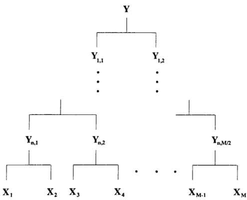
In various applications of the EM algorithm, it has been observed that in larger dimensional problems the speed of convergence of EM iterations considerably slows down [17, 18]. In order to improve the performance of the EM algorithm, several extensions of the basic EM steps have been proposed. In this thesis we provide further improvement on one of the extensions, the tree-structured EM (TSEM ), applied to the direction of arrival estimation of wide-band sig nals [16]. As showm in Figure 4.1, in TSEM. a multi-level tree-structured mapping between incomplete and complete data spaces is used. In this figure, the root, Y , denotes the observations (incomplete data) and the leaves, {X t }·, stand for complete data. The intermediate nodes, Yk,m·, are called intermediate incomplete data. We can summarize the computation involving intermediate incomplete data shown in Figure 4.2 as follows.
Let Yk,m an intermediate root, and and Yk+ij+\ be its leaves. When we reach this intermediate root during the run of TSEM, we compute Yk+\,j
u
Yn.,
X . X2 X j X4 Xm.i Xm
Figure 4.1: The binary tree structure between complete and incomplete data spaces for the case of number of signals M = 2"+^.
^k,m
^k+l,j+l
Figure 4.2: A detail from the binary tree structure.
as follows,
Yfc+lj — Yfc.m ~ ¿{k + 1, J + 1) s(0(A: + 1, ji + 1)) , (4.1)
where a{ k + l . j + l ) ’s and 0{k + 1,ji + 1 )’s are the amplitude and signal param eter estimates corresponding to the signals that form Yk+\j+\·, respectively. In other words, if we consider the section o f tree structure which is formed by Y jt+ij+i as root and the branches underneath, 1, j-|-l)’s and 1 . /-|-1) s will be the estimated parameters corresponding to the part of incomplete data which form the leaves of this section. After the computations are over for the branches under Yk+i,j (this means that the estimates corresponding to param eters of signals that form Yjt+ij have been computed), Y^+ij+j is evaluated in the same way by using the new values of a{k -f l , y ) ’s and 6{k -|- l , i ) 's . This switching between the intermediate leaves is performed for a prescribed num ber of times at each node. Note that, intermediate incomplete data at a node are updated each time a switching is performed at that node.
For example, as explained above, Yi^i in Fig 4.1 is computed in the following way:
M
Y .,i = Y - E t = ( M / 2) + l
(4.2)
where a,· and 9i are the current estimates o f the parameters. Y i,2 is also computed similarly with the new estimates of (á¿,^¿) for 1 < i < M /2 when the required steps are completed at each node beneath Y pi·
In this tree structure, the branches can be seen as hidden data spaces of the SAGE algorithm where only a subset o f algorithms are updated sequen tially [18]. Working in smaller dimensional spaces provides not only faster convergence but also higher computational savings since in the tree structure two signal components are treated at a time.
In order to further clarify the actual flow of operations, the steps of TSEM algorithm for the iterative estimation of 4 signal components are given below:
Y i,i = Y - ¿ i ? " ' s ( « y ' ) , (4.3)
t=3
a*] = E M ( Y i .i ,0 f - ’ , 0 ^ ' ) , (4.4)
Y.,2 = Y - i : a ? s ( « ? ) , 1=1
k-1 nk-l>
(4.5)
(4.6)
where llie iteration index /.■ starts from 0 and incremented until a stopi)ing cri terion is satisfied, and a^' are the estimates of parameters and amplitudes, respectively, at iteration. The function “EM” performs EM iterations stated through Eqns.(3.22)-(3.24) for two signals case (M = 2), by treating its first ar gument as observations and the remaining ones as initial parameter estimates. In order to use TSEM for the parameter estimation of more than four signal components, multi-level loops around the steps in Eqns.(4.3)-(4.6) are required. In the simulations, we provide results corresponding to 8 signal components by using only one additional loop. Note that, the application of TSEM is not required to power-of-2 signal components. When the number of signal com po nents is not power-of-2, the corresponding tree structure will not be a full one, and we may have to use EM algorithm to estimate only one signal component when there is only one leave emanating from the deepest nodes.
Chapter 5
Parameter Estimation of
Superimposed Exponentials in
Noise
The estimation of parameters of superimposed exponentials in noise is an im portant subclass of the general data model of Eqn.(2.1). The corresponding data model is:
M
¡,(n) = x ; + u (n ). (5.1)
t = l
where ^,’s are the prime parameters of interest and they can be com plex val ued. Although many sub-optimal estimation algorithms have been proposed for this application, Iterative Quadratic Maximum Likelihood (IQM L) algo rithm is the one providing exact ML estimates for the parameters [19]. In Appendix A, steps of the IQML algorithm, which exploits the exponential nature of the signal components for very efficient estimation of the signal pa rameters, are given. In the case of a few signal components, the performance of IQML algorithm is exceptionally well even for low SNR values and short data records. However, due to the complicated local maxima structure of the like lihood function, its performance degrades as the number of signal components
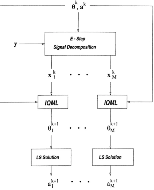
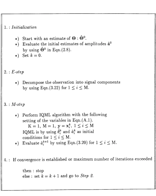
increases. The EM algorithm has been used in this application previously [21]. In our application of the EM and TSEM algorithms, we make use o f the IQML algorithm in the maximization step. Since, both EM and TSEM algorithms recjiiire ML estimates to be computed for a single signal component, by using IQ.ML algorithm to provide the required ML estimates, we obtained significant improvements in the efficiency of the EM and TSEM algorithms in this appli cation. The corresponding modification in the M-step of the EM algorithm is the replacement of the computation in Eqn.(3.23) with the IQML algorithm given in Appendix A. The steps of modified EM (IQML-EM) algorithm and the its block diagram are given in Table 5.1, and Figure 5.1, respectivelз^ The modification of TSEM is accomplished by using the IQML-EM algorithm in the Eqns.(4.4) and (4.6).
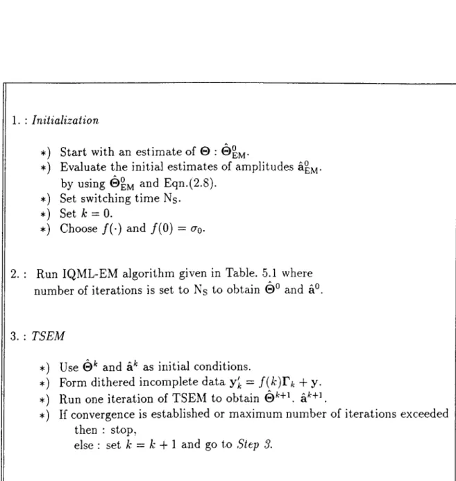
As it will be reported in the next chapter, even though TSEM converges faster than IQML-EM, it is more sensitive to the initial values of frequency parameters, 9^'s. In order to have a fast converging algorithm which is robust to the initial conditions, we propose Hybrid-EM algorithm where following a few IQML-EM iterations, TSEM algorithm is run, initialized with the final es timates of the IQML-EM iterations. Furthermore, in order to avoid converging to a potential local maxima, after switching to TSEM, additional noise whose variance is decreased during the iterations is added to the incomplete data. More explicitly, the incomplete data used in TSEM iterations is:
yi = y + /(O r ;,
(5.2)where / ( · ) is a monotonicaJly decreasing function with /( 0 ) = <7q, and F^’s
are independent sequence of random vectors with i.i.d. unit normal entries. This modification in TSEM iterations provides robust convergence, trading the speed of convergence. The steps of Hybrid-EM algorithm are given in Table 5.2.
k+1 • · · k+I
Figure 5.1: The block diagram of one iteration of IQML-EM algorithm.
*) Start with an estimate of 0 : 0 ° .
*) Evaluate the initial estimates of amplitudes a*’ by using 0 ° in Eqn.(2.8).
*) Set k = 0.
1. :
Initialization
2. : Estep
♦ ) Decompose the observation into signal components b}^ using Eqn.(3.22) for 1 < i < M.
3. ; M-step
*) Perform IQML algorithm with the following setting of the variables in E qn .(A .l).
K = 1, M = 1, y = X ,·, I < i < M
IQML is by using 6i and af as initial conditions for 1 < i < M.
*) Evaluate by using Eqn.(3.20) for 1 < ?’ < M.
4. : If convergence is established or maximum number of iterations exceeded
then : stop
else : set k = k + 1 and go to Step 2.
Table 5.1: The steps of IQML-EM algorithm whose Mstep is performed by IQML.
A ♦) Start with an estimate of © : ©em·
*) Evaluate the initial estimates of amplitudes by using ©EM Eqn.(2.8).
*) Set switching time Ns- *) Set /;: = 0.
*) Choose / ( · ) and /( 0 ) = <to
-1. :
Initialization
2. : Run IQML-EM algorithm given in Table. 5.1 where number of iterations is set to Ns to obtain © ” and a°.
3. : TSEM
*) Use ©^ and a^ as initial conditions.
:*=) Form dithered incomplete data =
f{k)Tk
+ y.*) Run one iteration of TSEM to obtain © '‘‘+U a*+U
*) If convergence is established or maximum number of iterations exceeded then ; stop,
else : set
k = k +
1 and go toStep 3.
Table 5.2: The steps of Hybrid-EM algorithm.
Chapter 6
Simulations
In this chapter, we present simulation based comparisons between IQML-EM, TSEM , and Hybrid-EM algorithms in terms of their convergence speed, sensi tivity to initial conditions, and accuracy. Also, the performance of these EM based algorithms are compared to the IQML algorithm and Cramer-Rao Lower Bound.
6.1
Simulation Set 1 : Case of Four Exponen
tial Signal Components
In the first part of this simulation set, we compare the sensitivities of IQML- EM, TSEM, and Hybrid-EM algorithms to the initial parameter estimat es. The incomplete data is formed as the superimposition of 4 sinusoids with frequency parameters, © = [0.18 0.32 0.52 0.40]"^, and amplitude parameters,
a =
[1.4 0.7 1.2 0.9]^, where the individual signal components are in the form of a.e·'"®·". The signal-to-noise ratio (SNR) is chosen to be 0 dB with thefollowing conventional SNR definition;
SNR = lOlogjo dB.
Parameter estimation error is defined as:
ee = ||e -© ||i
(
6
.
1
)
(
6
.2
) where 0 is the estimates of parameters. In order to investigate the sensitivity to the initial parameter estimates, the algorithms were run starting with 100different initial estimates each of which is chosen as:
0
° =
[ 6 i + V\ · · · 0 4+
1^4]^,
(6.3)where Vi’s are i.i.d. random variables which are uniformly distributed in the interval [—7, 7/]. We present here results obtained at two different values of
rj. The parameter estimation errors at the end of each run of algorithms are sorted and plotted for each algorithm including IQML. The results are dis played in Figures 6.1(a) and 6.1(b) for Tj = 0.055, and 0.1, respectively. As seen from Figures 6.1(a) and 6.1(b), in all the runs, IQML fails to converge to the error levels of the EM based algorithms. As seen in Fig. 6.1(a), for more precise initialization, TSEM, IQML-EM and Hybrid-EM converges to the de sired error level in approximately 82, 90 and 97 runs out of 100, respectively. As seen in Fig. 6.1(b), when the initial estimates are less accurate, out of 100 runs, the number of runs in which desired error levels are achieved decreases to approximately 57, 70 and 80 for the TSEM, IQML-EM and Hybrid-EM, re spectively. Hence, in contrast to its exceptional performance with fewer signal components, the IQML algorithm fails to converge to the parameter estima tion error levels of the EM based algorithms. Also, among the EM based algorithms, Hybrid-EM displays the lowest sensitivity to the initial estimates which is followed by EM and TSEM in that order. In order to have a fair com parison, each of the EM based algorithms are run until 60 iterative estimates are obtained for each frequency component. This corresponds to 60 iterations of the IQML-EM algorithm. For TSEM, in order to provide 60 iterations for each frequency component, we perform switching betw'een Y j,i and Y],2 af ter we perform 2 IQML-EM iterations at the bottom nodes. The switching between Y i,i and Y i,2 is performed 30 times. Based on our experience, per forming more switchings instead of performing more IQML-EM iterations at the bottom nodes provides better performance.
As we have mentioned before, Hybrid-EM has tw'o important parameters to be determined. One of them is the number of IQML-EM iterations performed prior to TSEM iterations. In this example we perform 8 IQML-EM iterations. It has been observed that within 8 iterations, IQML-EM algorithm pro\'ides a good estimate to at least one signal component. Also the monotonie decreasing function f{k ) in Eqn.(5.2) is chosen as:
f( k ) = e - ” ·“ , (6.4)
where k is the iteration count of the TSEM algorithm. Hence, with the 8
preliminary IQML-EM iterations and 26 TSEM iterations, in total 60 iterations for the Hybrid-EM are performed.
In order to compare the algorithms in terms of their speed of conver gence, the algorithms were run 20 times starting with the same initial es timates but with independent additive noise realizations. Also, to inves tigate the effect of SNR on the obtained results, this experiment was re peated at four different SNR values chosen as 5, 0, —5, and —10 dB, re spectively. All the EM based algorithms had the same set of parameters described earlier in this section. The initial estimates of frequency param eters are chosen as 0 ° = [0.16 0.30 0.54 0.42]^. The obtained results of the algorithms at SNR values 5, 0, —5, and —10 dB are shown in Fig ures 6.2(a), 6.2(b), 6.2(c), 6.2(d), respectively. As seen from these results, TSEM has faster speed of convergence than both IQML-EM and Hybrid-EM. which have about the same speed of convergence. Although all three algo rithms convergence to almost the same level of parameter estimation error at high SNR, they start to converge to different error levels for SNR values less than 0 dB. While TSEM and Hybrid-EM converge to more accurate re sults than IQML-EM, Hybrid-EM outperforms both of them at -1 0 dB SNR. This is because of the dithering used in the Hybrid-EM iterations which in creases the immunity of Hybrid-EM to local minima structure. This property of Hybrid-EM will be even more apparent in the next simulation set.
For the third simulation scheme of this part, all the values are kept con stant except for the initial estimates of frequency parameters. Initial con ditions are set to a value that is further away from real values than in the previous scheme as 6^ = [0.13 0.28 0.57 0.44]^. In the case of such initial estimates, TSEM fails to converge in most of the runs while the other two
converge. The obtained results of IQML-EM and Hybrid-EM are shown in Figures 6.3(a), 6.3(b), 6.3(c), 6.3(d), for 5, 0, —5, —10 dB SNR values, respec tively. As seen from these results, Hybrid-EM provides significantly improved estimates at SNR values lower than -5 dB. Hence, based on the obtained results, we can conclude that the Hybrid-EM algoritlnn is superior to the IQML-EM and TSEM algorithms in terms of both robustness to initial estimates and accuracy of the converged estimates.
By using the results given in Appendix B, we provide the comparison re sults of the EM based algorithms with the Cramer-Rao lower bound. As shown in Figure 6.4, for high SNR values all the algorithms have comparable perfor mances and they remain quite close to the Cramer-Rao lower bound. However as SNR value decreases, the accuracy of the algorithms starts to degrade with respect to the bound. The superiority of Hybrid-EM over the IQML-EM and TSEM is apparent in the low SNR case.
Finally, we present results on the obtained magnitude estimates by using the least-squares estimator given in Eqn.(3.20). In Fig. 6.5(a), comparison of EM based algorithms to the CRLB is shown. As seen from this figure, there is not much of a difference between the EM based algorithms in terms of their ac curacy in estimating the signal magnitudes. However, as seen from Fig. 6.5(b), TSEM converges faster than IQML-EM and Hybrid-EM algorithms. As com mented earlier, by using regularized estimators, biased but mean-square sense closer estimates to the amplitude parameters can be obtained [16].
(a)
(b)
Figure 6.1: Sorted resulting parameter estimation errors for 100 runs of IQML, IQML-EM, TSEM, and Hybrid-EM algorithms with different initial estimates determined by Eqn.(6.3). The figures in (a) and (b) correspond to 77 = 0.055 and
1
] = 0.1, respectively.(a)
(b)
(c) (d)
Figure 6.2: The tracks of average parameter estimation error of the IQML-EM, TSEM, and Hybrid-EM algorithms for (a) 5 dB, (b) 0 dB, (c) - 5 dB, and ^d) —10 dB SNR values. The initial estimates of frequency parameters were
0° = [0.16 0.30 0.54 0.42]"^.
(a) (b)
(c) (d)
Figure 6.3: The tracks of average parameter estimation error of EM and Hybrid-EM algorithms for (a) 5 dB, (b) 0 dB, (c) - 5 dB, a,nd (d) - 1 0 dB SNR values. The initial estimates of frequency parameters were
6^ = [0.13 0.28 0.57 0.44]T.
Figure 6.4: Frequency parameter estimation errors of IQML-EM, TSEM, and Hybrid-EM algorithms with Cramer-Rao lower bound.
(b)
Figure 6.5: (a) : Amplitude estimation errors of IQML-EM, TSEM, and Hy- brid-EM algorithms with Cramer-Rao lower bound, (b) : The track of average amplitude estimation error of IQML-EM, TSEM, and Hybrid-EM algoiithms for 0 dB SNR.
6.2
Simulation Set 2 : Case of Eight Expo
nential Signal Components
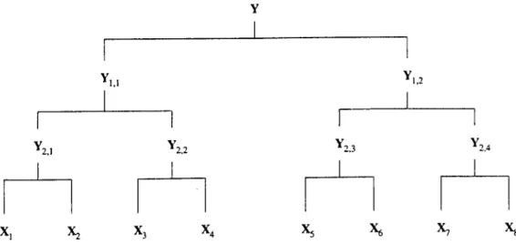
In this part, we provide comparison results between the estimation algorithms when the incomplete data has 8 superimposed exponential signal components. The TSEM and Hybrid-EM algorithms operated on the tree-structure shown in Fig 6.6.
Y
‘1,1 ' 1,2
2,1 ‘2,2 Y,2,3 2,4
X, Xz X3 X4 X5 X* X7 X*
Figure 6.6: Tree structured mapping in the case of 8 signals
The algorithms are run until 600 estimations are provided for each fre quency component. This corresponds to 600 IQML-EM iterations. The pro cedure for running TSEM has been decided as follows. At the bottom nodes, IQML-EM is run for 2 iterations, as in the case of previous part. Then the switchings between Y24 and Y2,2 (also between Y2,3 and Y2,-i) are performed
5 times. At the uppermost node, 60 switchings are performed. For Hybrid- EM, 40 IQML-EM iterations are performed prior to the TSEM iterations. Then, TSEM section of Hybrid-EM is implemented by making 56 switchings at the uppermost node while keeping the other parameters as the same as that of TSEM algorithm. Extra noise addition is implemented identically as in the previous simulation set. The frequency parameters of signals are set
to 6 = [0.25 0.18 0.30 0.35 0.45 0.40 0.56 0.50]^ and initial estimates
are chosen as 6^ = [0.23 0.20 0.28 0.37 0.43 0.41 0.54 0.48 The al gorithms are run for 20 different realizations at the same SNR levels as in the
previous simulation set. The averaged estimation errors as a function of it eration for each algorithm are shown in Figures 6.7(a), 6.7(b), 6.7(c), 6.7(d), for 5, 0, —5, —10 dB SNR values, respectively. As seen from the figures, tlie llybrid-EM algorithm has superior performance than both IQML-EM and TSEM. .A.lso, the IQML-EM algorithm yields the worst estimation error at its convergence. Based on these results, we conclude that as the number of signal components gets larger, the superiority of the Hybrid-EM over the IQML-EM and TSEM algorithms gets clearer.
(a) (b)
(c)
(d)
Figure 6.7: The tracks of average parameter estimation error of IQML-EM, TSEM, and Hvbrid-EM algorithms for (a) 5 dB, (b) 0 dB, (c) - 5 dB, and (d) - 1 0 dB SNr ' values. 0^ = [0.23 0.20 0.28 0.37 0.43 0.41 0.54 0.48]^ has been set as the initial parameter estimates.
Chapter 7
Conclusions and Future Work
For the maximum-likelihood estimation of superimposed parameters, Tree- Structured EM (TSEM) algorithm is proposed as an extension of conventional EM algorithm. Unlike the conventional EM, TSEM algorithm utilizes a binar}' tree structured multiple level mapping between the complete and incomplete data spaces. In order to investigate the performance of TSEM algorithm, an important special case of the general data model where the signal components are of exponential time functions is chosen as the test example. For this very well studied test case, we compared the performance of TSEM to those of IQML-EM and IQML algorithm. The IQML algorithm is a very efficient al gorithm which provides ML estimates to the parameters of exponential signal components [19]. However, the exceptional performance of IQML algorithm degrades considerably when there are more than four signal components. In the simulations, we observed that both IQML-EM and TSEM outperforms the IQML algorithm. It is also found that although TSEM converges faster than IQML-EM, it is more sensitive to the imprecision in the initial parameter estimates. In order to combine these desired features, we proposed a. Hybrid- EM algorithm which performs a few iterations on the initial estimates of the parameters and then TSEM iterations take over starting from the final esti mates provided by the IQML-EM iterations. Also, to provide more immunity to the local maxima structure of the likelihood surface, the incomplete data is
dithered with an additional white Gaussian noise whose variance exponentially decreased along with the iterations. It is found that as low as 8 IQML-EM it erations are sufficent to provide significant robustness to the initial estimates with a tolerable slowing down in the convergence compared to that of TSEM al gorithm. Based on extensive set of simulations, we conclude that Hybrid-EM is the algorithm of choice among IQML-EM, TSEM, and IQML algorithms. Furthermore, its performance improvement becomes more significant when the number of signal components gets larger or signal-to-noise ratio gets smaller.
As an extension of the work presented in this thesis, more reliable estimation of the amplitude parameters should be investigated. Since, in the proposed TSEM and Hybrid-EM algorithms, the signal amplitudes are estimated by- using a least-square estimator, the obtained results can be improved by using regularized least-squares estimators proposed in [16]. Furthermore, non-binary tree-structures can be used in TSEM with potentially even faster converging iterations. Finally, the proposed extensions of EM should be investigated in the absence of prior information in the noise statistics.
REFERENCES
[1] D. H. Johnson, and D. E. Dudgeon. Array Signal Processing. Prentice Hall, 1993.
[2] A. Bultan. A Four-Parameter Atomic Decomposition and the Related
Time-Frequency Distribution. Ph.D. dissertation. Middle East Technical
University, Dec. 1995.
[•3] J. A. Fessler, and .A. 0 . Hero. “Penalized maximum likelihood image- reconstruction using space alternating generalized EM algorithms,” IEEE
Trans, on Image Processing., vol. 4, pp. 1417-1429, Oct. 1995.
[4] S. Anderson, and A. Nehorai. “Analysis of a Polarized Seismic Wave Model,” IEEE Trans, on Signal Processing, vol. 44, pp. 379-386, Feb. 1996.
[5] C. Esmersoy, V. F. Cormier, and M. N. Toksoz. “Three-component array processing,” the VELA program, A Twenty-Five Year Review of Basic Research. Dianne L. Carlson, 1985. Library of Congress Catalog Card Number : 85-080931. pp. 565-578.
[6] Y. T. Chan, J. M. Lavoie, and J. B. Plant. “A parameter estimation ap proach t o e s t i m a t i o n o f frequencies of sinusoids,” IEEE Trans, on Acoust.,
Speech, Signal Processing, vol. ASSP-33, pp. 214-219, Apr. 1981.
[7] M. R. Matausek, S. S. Stankovic, and D. V. Radivic. “ Iterative inverse filtering approach to the estimation of frequencies of noisy sinusoids,”
IEEE Trans, on Acoust., Speech, Signal Processing, vol. ASSP-31, pp.
1456-1463, Dec. 1983.
[8] S. M. Kay. “Accurate frequency estimation at low signal-to-noise ratio,”
IEEE Trans, on Acoust., Speech, Signal Processing, vol. ASSP-32. pp.
540-547, Jun. 1984.
[9] P. Dempster, N. M. Baird, and D. B. Rubin. “Ma.ximuni likeliliood from incomplete data via the EM algorithm,” J. Roy. Slat. Soc., vol. B-39. pp. 1-37, 1977.
[10] S. C. Chen, T. J. Schaiewe, R. S. Teichman, and M. I. Miller. “Parallel algo rithms for maximum likelihood nuclear magnetic resonance spectroscopy,”
J. Magn. Resonance, Mar. 1993.
[1 1] M. I. Miller, and A. Greene. “Maximum-likelihood estimation for nuclear magnetic resonance spectroscopy,” J. Magn. Resonance, vol. 83. pp. 525- 548, 1989.
[12] M. I. Miller, and D. R. Fuhrmann. “Maximum likelihood narrowband direction finding and the EM algorithm,” IEEE Trans, on Acousi., Speech,
Signal Processing, vol. ASSP-38, pp. 1560-1577, Sep. 1990.
[13] M. Feder, and E. Weinstein. “ Parameter estimation of superimposed sig nals using the EM algorithm,” IEEE Trans, on Acoust., Speech, Signal
Processing, vol. 36, pp. 477-489, 1988.
[14] R. A. Boyles. “On convergence o f the EM algorithm,” J. Roy. Slat. Soc.,
vol. B-45, pp. 47-50, 1983.
[15] C F. J. Wu. “On the convergence properties of the EM algorithm,” The
Annals of Statistics, vol. 11, pp. 95-103, 1983.
[16] N. (^adalli, and 0 . Ankan. “Wide-Band Maximum Likelihood Direction Finding and Signal Parameter Estimation by Using the Tree-Structured E.M Algorithm,” submitted to IEEE Trans, on Signal Processing.
[17] M. Segal, and E. Weinstein. “The cascade EM algorithm,” Pi'oc. IEEE,
vol. 76, pp. 1388-1390, Oct. 1988.
[18] J. A. Fessler, and A. 0 . Hero. “Space alternating generalized expectation- maximization algorithm,” IEEE Trans, on Signal Processing, vol. 42, pp. 2664-2677, Oct. 1994.
[19] Y. Breşler, and A. Macovski. “Exact maximum likelihoood parameter estimation of superimposed exponential signals in noise,” IEEE Trans,
on Acoust., Speech, Signal Processing, vol. ASSP-34, pp. 1081-1089, Oct.
1986.
[20] A. Papoulis. Probability, random variables and stochastic processes. Mc- Graw Hill, 1991.
[2 1] M. J. Turmon, and M. I. Miller. “ Maximum-likelihood estimation of com plex sinusoids and toeplitz covariances” , IEEE Trans, on Signal Process
ing, vol. 42, pp. 1074-1086, May 1994.
[22] T. M. Cover, J. A. Thomas. Elements of Information Theory. John Wiley
Sz Sons, 1991.
[2-3] L. L. Scharf. Statistical Signal Processing. Prentice Hall, 1991.
A P P E N D IX A
Iterative Quadratic Mciximum
Likelihood (IQML) Algorithm
For very efficient computation of ML estimates to the parameters of super imposed exponential signals in Gaussian noise, the IQML algorithm has been proposed [19]. The IQML provides estimates to both the amplitude, a,„,, and phase, 9i and fii, parameters in the following model:
M
y „(n ) = 0 < n < N - 1, 1 < m < K . (A .l) t = l
IQML algorithm consists of the following steps.
1. Initialization : k = 0, and = bo, e.
2. Form the data matrix:
y m ( M ) y „ , ( M - l ) ym(M + 1) ym(M) Ym = ym(0) ym(l) y m ( N - l ) y , „ ( N -2) ··· t / „ ( N - M - l )
37
3.
Form the coefficient matrix:
0 0 0 0 r{k) 0 0 and computeK
m = l (A .2)4. Update the coefficient vector:
_ arg min |b^Cy ^b| .
5. If llb^'·"'·^) — b^^'^ll < e, then go to Step 6, otherwise go to Step 3.
(A.3)
6. Compute the roots of which is a poljmomial whose coefficients are the entries of The obtained roots are equal to } for
1 < ?: < M.
A P P E N D IX B
Cramér-Rao Lower Bound
Here we provide the CRLB for the following superimposed sinusoidal signal model:
M
y{n) = '£ a .e ^ ” "' + u{n},
(B .l)t = l
where u[n) is zero mean i.i.d. Gaussian noise with variance cr^. Then the corresponding log-likelihood of observations is given as:
N - l M
£(Í7; y ) = K + — ^ y{n) - JTT^.n
n = 0 1=1
^ » ( n ) j , (B.2)
where K denotes the constant terms, is [ 0 a]"^, and * denotes conjugation. The Cramer-Rao bound sets a lower bound on the error covariance of the esti mator and it is found by inverting the Fisher information matri.x which is equal to the covariance matrix of the score function [2.3]. The score function is eval uated by taking the partial derivatives of log-likelihood function with respect to the parameters. Hence the score function is found as follows. First, com pute the partial derivative of the log-likelihood with respect to the frequency- parameters:
dOm
1 N - i Í / M \ *
M
+ I , (B.3)
where Q „(n ) = ( a „ j7rn)e^'’^®"·". By defining A (??) = [q i(?7.) 02(0) ··· a-M(n)]'^,
we get
a c { i ^
= ^ ¿ | A ( n ) ^ ! , ( n ) - g < i i e ’ '''"j
+ A - ( n ) ^ y { n ) - f ; o . e ' " ' " j | . (B .4) Similarly, compute the partial derivative of the log-likelihood with respect to the amplitude parameters
da
a £ ( i2;y ) ^
+
fimi") (y{’>) - Y.
I ,
(B.5)where /3min) = By defining B(?j) = [li\{n) /?2(??) ··· we get:
+ B '(n ) ly{n) - I . (B .6) Hence, if we define C (n) = [A(n) B (n)]^, we can write d C jd ^ as:
a £ ( n ; y ) 1 i ri=0 [ d n , N - l r / M \ * = ^ E I C(i?) |^y(77.) -(B.7)
which is the score function. The Fisher information matrix is given by:
Since the additive noise is white, the Fisher information matrix is found as:
J ( ii) = ^ E (C (n )C »(n .) -f C*(n)CT(,7.)) . (B.9) ___n
Hence, the Cramer-Reio lower bound is found as follows
/N-1 \ - i
CRLB(ii) = (C(ir)C»(n) + C*(n)CT(n)) j (B.IO)