rtPS uplink scheduling algorithms for IEEE 802.16 networks

rtPS Uplink Scheduling Algorithms for IEEE

802.16 Networks

M. Cenk Erturk1,2_{, Nail Akar}1_{, Member, IEEE}

1_{Department of Electrical and Electronics Engineering, Bilkent University,}

TR-06800 Bilkent, Ankara, Turkey

2_{Defense and Security Research Group, the Scientific and Technological Research Council of Turkey,}

Kavaklidere 06100, Ankara, Turkey Abstract - IEEE 802.16 MAC provides flexible bandwidth

allocation and QoS mechanisms for users with different requirements. However, QoS scheduling is not specified by the 802.16 standard and is thus left open for vendors’ implementation. In this paper, we propose an uplink scheduler to be used in WiMAX Base Station (BS) for rtPS type of connections. We propose that the base station maintains a leaky bucket for each rtPS connection to police and schedule rtPS traffic for uplink traffic management. The proposed scheduler is studied via simulations in MATLAB and throughput and fairness properties of the scheduler are demonstrated.

I. INTRODUCTION

EEE 802.16, the so called WiMAX, is the standard developed for the MAC and physical layers for broadband wireless metropolitan area networks. The standardization of WiMAX began in 1999 and the first standard is published in 2001. Several amendments i.e. 802.16 2001, 802.16a, 802.16c are introduced but IEEE 802.16d 2004 standard [1] revises and consolidates all up to 2004. IEEE 802.16d 2004 (fixed WiMAX), IEEE 802.16e 2005 [2] (mobile WiMAX) are the most widely used standards for WiMAX. The most recent amendment 802.16e considers issues related to mobility and scalable OFDMA in addition to given features in fixed WiMAX.

IEEE 802.16 standard offers two operational modes: point-to-multipoint (P2MP) or mesh modes. In P2MP mode, Subscriber Stations (SS), e.g., laptops, PDAs or access points communicate with other SSs via a Base Station (BS) whereas in mesh mode SSs can communicate with each other without a need for BS. Most of current research on WiMAX systems focuses on the simpler P2MP mode which will also be the scope of this paper.

Data transmissions are frame based in WiMAX. Frame durations are fixed and partitioned into a number of slots. A slot can be defined as the smallest time and frequency unit of a frame that can be allocated for transmission. A frame is partitioned into downlink (DL) (BS to SS) and uplink (UL) (SS to BS) subframes. BS controls the contents of subframes

in terms of scheduling via UL and DL MAP messages. In addition, there are also messages defined for synchronization, ranging, activation of connections, service flow changes, etc in [1] and [2]. As far as this paper is concerned, we only focus on the DL MAP and UL MAP messages. The scheduling problem for the downlink where the backlog of each SS is known by the BS is not much different than scheduling problems for wireline networks; therefore, our focus in this study is the uplink scheduling problem.

IEEE 802.16 subframes can be duplexed either by Frequency Division Duplexing (FDD); transmissions in each subframe can occur at the same time but at different frequencies, or by Time Division Duplexing (TDD); transmissions in each subframe can occur at the same frequency but at different times. SSs can be full duplex (transmit and receive simultaneously) or half duplex (either transmit or receive in certain time). Most systems use TDD which will be the scope of this paper.

Bandwidth requests are always per connection but WiMAX standard specifies two allocation modes to those requests: grant per connection (GPC) or grant per SS (GPSS). The latter mode requires a further scheduling unit at the SS so as to reallocate the granted bandwidth to the connections which belong to the same SS [7]. We do not differentiate between these two grant allocation modes in this paper since we assign only one connection to each SS.

There are five service classes defined in the standard [2]: Unsolicited Grant Service (UGS), real-time Polling Service (rtPS), extended real-time Polling Service (ertPS), non-real-time Polling Service (nrtPS) and Best Effort (BE). UGS is designed to support Constant Bit Rate (CBR) applications and real-time service flows that generate fixed-size data packets on a periodic basis such as Voice over IP (VoIP) without silence suppression. On the other hand, rtPS is designed to support real time applications with variable size packets and with periodic nature such as compressed voice, video conferencing, Video on Demand (VoD). The ertPS service class is built on the efficiency of both UGS and rtPS and it is designed for real time traffic with variable data rate in an

on-I

Proceedings of Eighth International Symposium on Computer Networks (ISCN’08) ISBN: 978-975-518-295-7, Copyright ©2008 by Boğaziçi University

off manner such as VoIP with silence suppression. For data, the nrtPS class is designed to support non real time variable packet size applications such as File Transfer Protocol (FTP) but with QoS guarantees in terms of bandwidth per connection. BE is designed for applications that do not require any QoS commitments such as ordinary WEB surfing. Table 1 summarizes these five QoS classes and their parameters. In particular, in the rtPS service, the BS provides periodic unicast bandwidth request opportunities to the rtPS connections. Using these opportunities, the SSs send their bandwidth requests to the BS and they do not use contention request opportunities. Some of the key mandatory traffic parameters for the rtPS service class that are key to our work are Minimum Reserved Traffic Rate (MRTR) (in bps), Maximum Sustained Traffic Rate (MSTR) (in bytes per frame), and Maximum Latency (ML) (in seconds).

MRTR specifies the average bandwidth commitment given to the connection over a large time window. On the other hand, MSTR determines the maximum number of bytes an SS can request in one single frame. The parameter ML specifies the maximum latency between the entrance of a packet to the Convergence Sublayer of the MAC and the epoch at which the corresponding packet is forwarded to the WiMAX air interface [2]. A good rtPS implementation is to ensure the QoS requirements of all rtPS connections including those that are negotiated at connection setup for example MRTR, MSTR, and ML. The goal of this paper is to design an rtPS scheduler for uplink traffic for IEEE 802.16 WiMAX networks.

Table 1

TRAFFIC PARAMETERS FOR SERVICE CLASSES

Class Minimum rate

Maximum rate

Latency Jitter Priority

UGS X X X

rtPS X X X X

ertPS X X X X X

nrtPS X X X

BE X X

The organization of this paper is as follows. Section 2 addresses a brief overview of 802.16 PHY and MAC layers. The MAC layer parameters together with the proposed scheduler are presented in Section 3. Section 4 presents the simulation results. Section 5 concludes and gives a roadmap for future studies.

II. IEEE802.16OVERVIEW

Both fixed and mobile WiMAX standards do not specify the carrier frequency (2-11 GHz) and define general limits for channel sizes (1.25 – 20 MHz). Since neither worldwide spectrum band is allocated nor committed channel size is defined, WiMAX forum (www.wimaxforum.com) defines system profiles for interoperability. Mobile WiMAX System Profile Release 1 is defined as follows: IEEE 802.16 2004, IEEE 802.16e and some optional and mandatory features. In Release 1, Mobile WiMAX profiles will cover 5, 7, 8.75, and 10 MHz channel bandwidths for licensed worldwide

spectrum allocations in the 2.3 GHz, 2.5 GHz, 3.3 GHz and 3.5 GHz frequency bands, the latter of which is the most widely available band from the whole spectrum (except for US). The channel sizes for this frequency band is therefore integer multiples of 1.75 MHz, i.e., 1.75 MHz, 3.5 MHz, 7MHz, 8.75 MHz, etc.

A. OFDM vs. OFDMA

IEEE 802.16 specifies two types of Orthogonal Frequency Division Multiplexing (OFDM) systems: OFDM and Orthogonal Frequency Division Multiple Access (OFDMA).

OFDM is a multi-carrier transmission technique that has been recently recognized as a method for high speed bi-directional wireless data communication. Frequency Division Multiplexing (FDM) scheme uses multiple frequencies to transmit multiple signals in parallel. In FDM, the allocated spectrum is broken up into several narrowband channels known as “subcarriers”. In FDM, frequency bands for each signal is disjoint, therefore, the receiver demodulates the total signal and separates the bands using filters. In OFDM, the subcarriers are overlapping. Since the subcarriers are

orthogonal to each other, there is no interference between

each data carrier [4].

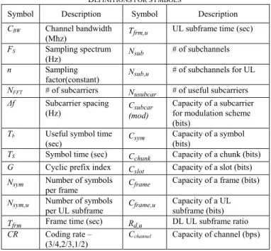
Table 2 DEFINITIONS FOR SYMBOLS

Symbol Description Symbol Description

CBW Channel bandwidth

(Mhz) Tfrm,u

UL subframe time (sec)

FS Sampling spectrum (Hz) Nsub # of subchannels n Sampling factor(constant) Nsub,u # of subchannels for UL

NFFT # of subcarriers N_usubcar # of useful subcarriers

Δf Subcarrier spacing

(Hz) C_(mod) subcar

Capacity of a subcarrier for modulation scheme (bits)

Tb Useful symbol time

(sec) Csym

Capacity of a symbol (bits)

TS Symbol time (sec) _Cchunk Capacity of a chunk (bits)

G Cyclic prefix index _Cslot Capacity of a slot (bits)

N_sym Number of symbols

per frame Cframe

Capacity of a frame (bits)

N_sym,u Number of symbols

per UL subframe Cframe,u

Capacity of a UL subframe (bits)

T_frm Frame time (sec) R_d,u DL UL subframe ratio CR Coding rate –

(3/4,2/3,1/2)

Cchannel Capacity of channel (bps)

Each subcarrier can be modulated with Binary Phase Shift Keying (BPSK) (Csubcar(BPSK)=1bit), Quadrature Phase Shift

Keying (QPSK) (Csubcar(QPSK)=2bits), 16 Quadrature

Amplitude Modulation (16QAM) (Csubcar(16QAM)=4bits) or

64 Quadrature Amplitude Modulation (64QAM) (Csubcar(64QAM)=6 bits) technique.

In OFDM PHY there are a number of subcarriers spanning the sampling spectrum, meaning OFDM modulation can be realized with Inverse Fast Fourier Transform (IFFT). The standard [1] defines the number of subcarriers as 256. It is important to note that in IEEE 802.16 2004 subcarriers cannot

be allocated for different users i.e. subchannelization which is to group subcarriers, is not defined; therefore in terms of scheduling, according to 802.16 2004 minimum allocation unit of a frame is simply one OFDM symbol for downlink. 802.16 2004 allows up to 16 subchannels for uplink. For the OFDMA case, standard [1], [2] defines that a group of subcarriers can be assigned for different users for both uplink and downlink. Scalable OFDMA introduces fixed subcarrier spacing, which is equal to 10.94 kHz [3], therefore the number of subcarriers is variable (up to 2048) and symbol durations are fixed.

8000 8000 ⎥⎦× ⎥ ⎢⎣ ⎢ × = BW s C n F (1) FFT s N F f = Δ (2), Tb _f Δ = 1 (3) For multipath channels, to cope with channel delay spreads

and time synchronization errors a paradigm called cyclic prefix (CP) is introduced [4]. Therefore overall symbol time can be defined as follows:

G T T T_S= _b+ _b× (4) where, G=0.5m,m∈

_{

}

(

)

It can be seen from Eq. (5) that, there can be a gap at the end of the frame, if the symbol time is not a multiply of frame time. Since there can not be data transmission in this gap, it can be defined as an overhead.

FFT usubcar N

N = ×

128

96 ₍₆₎

It can be seen from Eq. (6) that number of useful subcarriers is not equal to the number of subcarriers. Since, for example in OFDM, we have totally 256 subcarriers but not all of these subcarriers are energized. There are 28 lower, 27 upper guard subcarriers and a DC subcarrier that are never energized. Also there are 8 pilot subcarriers that are dedicated for channel estimation purposes. Therefore only 192 data subcarriers are left for data transmission [4]. For the OFDMA case where number of subcarriers varies between 128 – 2048, number of useful subcarriers can be calculated with Eq. (6). In order to calculate the capacity of a chunk (the minimum frequency time unit of a frame), we first need to calculate the capacity of a symbol.

CR C

N

C_sym= _usubcar× _subcar× (7)

sub sym chunk C N

C = / (8) A chunk can be defined as the minimum allocation unit i.e. slot for the OFDM uplink case but for downlink case Cchunk is

simply equals to Csym since subchannelization is not available

in downlink. However for OFDMA case it is defined that, for downlink Fully Utilized Subchannels (FUSC) a slot is (1 subchannel) x (1 OFDMA) symbols, for downlink Partially Utilized Subchannels (PUSC) 1x2, for uplink PUSC 1x3 and for downlink and uplink adjacent subcarrier permutation 1x1.

Therefore calculation of the capacity of a frame and capacity of the channel is:

(

)

frame N N C C = × × (9) frm frame channel _T C C = (10) The effect of Eq. (7) to Eq (10) shows that modulation type and coding rate of SSs directly affect the channel overall capacity. To calculate uplink channel capacity, one should replace Tfrm with Tfrm,u in Eq. (5) and follow Eq. (5-10) with

new parameter where,

(

)

frm u

frm T R

T _, = ×1− _, (11) III. CAPACITY PLANNING AND SIMULATION ENVIRONMENT In this section, we explain the scheduling polices and the environment. Capacity plans for the simulation types and traffic of connections are also discussed.

A. Simulation Environment

All simulations are implemented in MATLAB and run for 20 seconds duration. We study the uplink scheduling problem but our scheduling proposal can be extended to downlink scheduling.

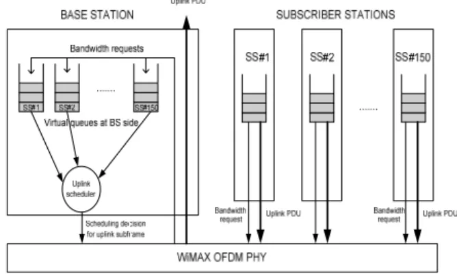
Not all the procedures and functions of WiMAX environment are implemented; since this study is a concept demonstration and the scope of this paper is basically on uplink scheduler and frame. DL and UL MAP messages are assumed to be sent in the downlink frame. There is no loss or overhead due to channel conditions and CRC field is not implemented in the simulation. The service class chosen is rtPS and WirelessMAN OFDM is the physical layer of the system. Fig. 1 defines the environment in terms of functions defined for BS and SS’.

Fig. 1 Uplink Functions within BS and SSs.

B. Capacity Planning Parameters

Capacity of an OFDM system can be calculated via Eq.(1– 11). Selected and calculated parameters are given in Table 3.

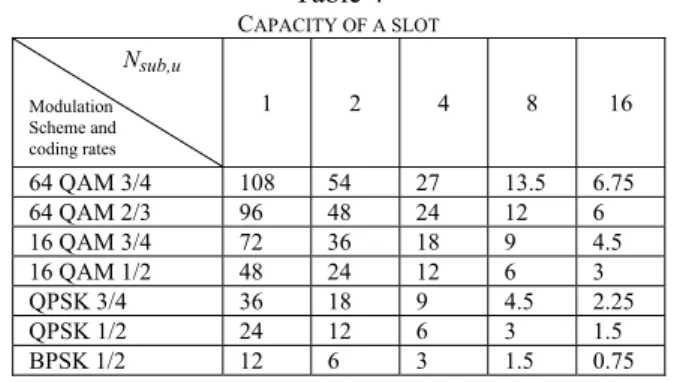
Capacity calculation for the overall system depends on the modulation scheme and coding rates of connections. Via Eq. (7-8) the capacity of a slot can be calculated. It is important to note that we assume one chunk is defined as one slot. The

capacity of a slot (in bytes) for various modulation schemes, coding rates and number of subchannels are given in Table 4.

Table 3

PARAMETERS FOR SIMULATION

Parameter Value Description

CBW 7 MHz Selected

FS 8 MHz Calculated via (1)

N 8/7 8/7 for CBW multiple of 1.75 MHz in OFDM.

NFFT 256 Defined by [1] Δf 31250 Hz Calculated via (2) Tb 32 us Calculated via (3) G 1/16 Selected TS 34 us Calculated via (4) Tfrm,u 2.5 ms Selected Nsym,u 73 Calculated via (5)

Nsub,u 8 Selected

Nusubcar 192 Calculated via (6)

Nslot 584 Nsym,u x Nsub,u (# of slots in a frame)

The capacity of a frame (using Eq. (6)) changes from 7884 bytes (for 16 QAM 3/4) to 876 bytes (for BPSK 1/2) therefore via Eq. (10); capacity of channel varies between 25.2 Mbps and 2.8 Mbps. Table 4 CAPACITY OF A SLOT Nsub,u Modulation Scheme and coding rates 1 2 4 8 16 64 QAM 3/4 108 54 27 13.5 6.75 64 QAM 2/3 96 48 24 12 6 16 QAM 3/4 72 36 18 9 4.5 16 QAM 1/2 48 24 12 6 3 QPSK 3/4 36 18 9 4.5 2.25 QPSK 1/2 24 12 6 3 1.5 BPSK 1/2 12 6 3 1.5 0.75 C. Traffic Related Parameters

The traffic pattern used in all scenarios is the modified version of near real time video streaming model defined in [8]. The main reason for this choice is that this traffic pattern has variable packet lengths and random packet inter-arrival times; therefore is suitable for the rtPS class.

The video streaming model is frame based and generates a deterministic number of variable length packets in a video frame. The traffic model parameters are given in Table 5. The mean of the generated traffic per SS, denoted by r is 64 kbps and can be calculated via Table 5.

Table 5

PARAMETERS FOR TRAFFIC MODEL

Component Distribution Parameters

Inter-arrival time between the beginning of each frame

Deterministic 100ms Number of packets in a

frame

Deterministic 8 packets per frame Packet size Truncated Pareto Mean = 100 Bytes

Min = 40 Bytes Max = 250 Bytes Inter-arrival time between

packets in a frame

Truncated Pareto Mean = 6 ms Min = 2.5 ms Max = 12.5 ms

D. Scheduling Policies

The BS scheduler assigns slots to the SSs. SSs send their bandwidth requests to the BS in response to the unicast polls.

Fig. 2 Uplink Scheduler

Since we assume neither fragmentation nor packing is enabled, the requests result either with a whole grant for each request or nothing. Therefore, the length of the bandwidth request becomes a critical issue, since there is a higher probability that small requests fit into the frame; on the other hand SS’ which sent larger requests have opportunity to send more from their backlog. This tradeoff and the choice of optimal bandwidth request size is not considered in this study.

BS scheduling is done in the following manner for every frame:

1-Depending on the initial negotiation by each SS which determines how frequently unicast polling is done, first, BS assigns unicast polling slots to each SS. The modulation scheme and coding rate of SSs determines the slot size in bytes. According to their slot size, the number of unicast polling slots are calculated and assigned to each SS. For example, for a slot size of 6 bytes, one slot is sufficient for bandwidth requests since the request’s MAC header is 6 bytes without the CRC field. Unicast polls are assigned to each user depending on their bandwidth request index (BRI). When BRI is n for an SS, then unicast polling for that SS is done once in every n frame.

2- The BS maintains a leaky bucket of a certain size B for each SS (Fig. 2). When a SS has the chance to send its requested data in a certain frame, then the bucket is incremented by the length of the granted data. Moreover, the bucket leaks in each frame by a number of bytes dictated by the connection’s MRTR. When a bandwidth request message arrives at the BS, and the sum of the current bucket value and the new bandwidth request exceeds the bucket limit B; then the bandwidth request is marked ‘illegitimate’.

3- Let τi and Si denote slot size (in bytes) and bandwidth

request (in bytes) of ith _{SS respectively. Then;}

⎥ ⎥ ⎤ ⎢ ⎢ ⎡ = i i i S τ T

where Ti is the bandwidth request of the ith SS in number of

slots.

4-Let L is set of the SSs whose packets are legitimate. slot L i i N T <=

∑

a) Schedule slots for the set L. It is important to note that there can be additional slots not assigned to any SS. This may happen for two reasons: First is that there may be no packets in SS’ virtual queue at BS side, second, their bucket may be full therefore they may not be eligible for bandwidth assignment in this frame.

Those slots (

∑

∈ − L i i slot T N

parameter for each SS is satisfied. Remaining slots are eligible for all SSs and should be distributed fairly among all users in a round robin manner. Moreover, to maximize the throughput, these slots can be assigned for the SS’ having higher modulation schemes and coding rates.

b) Schedule the first K legitimate SS’ backlog such that

slot K i i N T

∑

but . And search through the rest of

slot K i i N T

∑

SSs in order to schedule other SS’ packets that would fit into remaining bandwidth. In addition, first K SS’ are changed in each frame in a round robin manner in order to ensure the fairness.

IV. SIMULATION RESULTS

In this section, we present and discuss the results of simulations. In all simulation scenarios there are one BS and 150 SSs generating traffic according to near real time video streaming model. Therefore, offered traffic to the system is 150x64kbps=9.6Mbps.

All simulations are done within the same environment given in Fig. 3.

Fig. 3 Simulation Environment

Minimum reserved traffic rate (MRTR) for the first 100 of 150 SS is 68kbps, 64kbps for data and 4kbps for MAC header overheads. The last 50 SS has MRTR of 10 kbps. The reason for these choices is to prove that the scheduler protects the SS’ having larger MRTR parameter. Maximum sustained traffic rate (MSTR) parameter is chosen as 500 bytes per frame. Maximum Latency for a video frame (100ms) is 500 ms i.e. if a video frame is not sent within 500ms SS simply drops the entire video frame (8 packets).

A. Simulation Scenario 1

In this scenario BS always sends unicast poll for each and every SS in every frame so that BS learns the requests of each user immediately after the packets are generated by SSs. All

SSs in this scenario use 16 QAM 1/2, therefore the capacity of a slot is 6 bytes, the capacity of a frame is 3504 bytes and capacity of channel is 11.21 Mbps. But since 150 slots are assigned for bandwidth requests there are 434 (584-150) slots available for data transmission; the available capacity for data transmission becomes 2604 bytes (8.33 Mbps) in a frame. It is important to note that after satisfying all SS’ MRTR parameter (100x68kbps+50x10kbps=7.3 Mbps), there exists a remaining bandwidth.

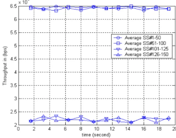
Fig. 4. Throughput for 150 SS.

Fig. 4 shows that all SSs have the throughput of their MRTR parameter. BS scheduler protects the first 100 SSs from the rest which offer higher traffic from their MRTR. In this scenario the useful throughput of the system is 7.485 Mbps, overheads due to bandwidth request headers, MAC headers, not fitting of bandwidth requests to a number of slots (because of ceiling Ti) and the unused slots are 2.88 Mbps,

0.447 Mbps, 0.152 Mbps and 0.247 Mbps respectively.

B. Simulation Scenario 2

Second simulation is done to prove that less aggressive bandwidth request mechanisms will increase the throughput. In this scenario SS’ do not send their bandwidth request in each frame i.e. unicast polling is not done on a frame by frame basis but once in every three frame i.e. mean interarrival times of packets in the video streaming model is 6 ms. SSs MSTR, MRTR, ML, slot size and traffic paterns are same with Scenario 1. Fig. 5 shows that since bandwidth request mechanism is less aggressive, there are more slots for data transmissions; the number of remaining slots is increased and these are assigned mostly to the last 50 SSs. In this scenario the useful throughput of the system is 9.23 Mbps, overheads due to bandwidth request headers, MAC headers, not fitting of bandwidth requests to a number of slots (due to ceiling Ti) and the unused slots are 0.96 Mbps, 0.55 Mbps,

0.08 Mbps and 0.37 Mbps respectively.

Fig. 5. 150 SS Less Aggressive Bandwidth Requests.

C. Simulation Scenario 3

In this scenario we prove that the choice of Bandwidth Request Index (BRI) is very important to maximize the throughput of overall system. QoS parameters, simulation environment and traffic choices are the same with Scenarios 1 and 2, however, in this scenario MRTR parameter is not assigned to SSs. Every SS in the system is said to be equal in terms of bandwidth assignments. It is obvious that when bandwidth request index is set to mean of inter-arrival times of packets, the overall throughput will be maximized but this may not be the case for some scenarios since unicast polling can be done for only multiplies of frame duration. Fig. 6 presents the overall throughput for variable choices of BRI.

Fig. 6 Overall Throughputs for various BRI

D. Simulation Scenario 4

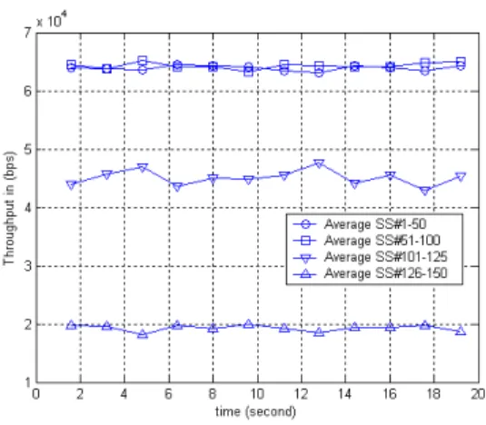
In this scenario we propose that slot sizes of SSs do not affect the system in terms of QoS. Bandwidth request is per frame and slot sizes are 9, 6, 9 and 3 bytes for SS’ 1-50, 51-100,101-125,125-150 respectively.

Fig 7. shows that after satisfying all SS’ MRTR, when compared with Fig 4., there remains more remaining bandwidth assigned to last 50 SSs in this scenario. The main reason is that SS#1-50 and SS#100-125 has a greater slot size of when it’s compared to Scenario 1, meaning that they need less number of slots to ensure their MRTR parameter.

Fig. 7. 150 SS Different Slot Sizes

Fig. 7 also shows that SS#101-125 have higher throughput compared to SS#126-150. The remaining slots are distributed fairly among SSs but since SS#101-125 have greater slot sizes their throughput is higher.

E. Simulation Scenario 5

In the last scenario, bandwidth requests and slot sizes are the same with Scenario 4, but this time BS assigns remaining slots firstly to the SSs having greater slot sizes (priority parameter), to increase the overall throughput. Fig. 8 shows that the remaining bandwidth is firstly distributed between SS #101-125 and then what remains is distributed between SS #126-150. The mean of overall throughput is 8.01 Mbps in Scenario 3; whereas in this scenario the mean of overall throughput is 8.32 Mbps.

Fig. 8. 150 SS Different Slot Sizes and Priority

V. CONCLUSION

This paper presents channel design criterias in WiMAX for OFDM/OFDMA systems. The results show that BS protects SSs who need higher Minimum Reserved Traffic Rate parameters from other SSs which offer traffic to the system much above of their MRTR parameter. Bandwidth request mechanisms are important in terms of increasing throughput

for IEEE 802.16 environments. It is shown that slot sizes of SS’, which depend on modulation schemes and coding rates of them, also affect the system throughput. It is proven that presented scheduling mechanism satisfies the QoS parameters of SSs no matter what their slot sizes are. Finally, it is shown that after satisfying all other service class parameters, making opportunistic scheduling for remaining slots for those connections which have greater modulation schemes increases the overall throughput. The future direction of this study will be on latency measurements of rtPS class traffics. Fair and opportunistic bandwidth allocations when channel conditions are variable during the simulation time will be studied in details.

ACKNOWLEDGMENT

This work is part of a project that has been funded by the Scientific and Technological Research Council of Turkey under Grant Number 106E046.

REFERENCES

[1] Air Interface for Fixed Broadband Wireless Access Systems, IEEE Standard 802.16, June 2004.

[2] Air Interface for Fixed Broadband Wireless Access Systems – Amendment for Physical and Medium Access Control Layers for Combined Fixed and Mobile Operation in Licensed Bands, IEEE Standard 802.16e, December 2005.

[3] Mobile WiMAX – Part I: A Technical Overview and Performance

Evaluation, www.wimaxforum.org, 2006.

[4] J.G.Andrews, A. Ghosh and R. Muhamed, "Fundamentals of WiMAX-understanding Broadband Wireless Networking", Prentice Hall, Feb, 2007

[5] Mark C. Wood, An Analysis of the Design and Implementation of QoS

over IEEE 802.16,

http://www.cse.wustl.edu/~jain/cse574-06/ftp/wimax_qos/index.html, 2006.

[6] Sayenko, O. Alanen, J. Karhula, T. Hamalainen, “Ensuring the QoS Requirements in 802.16 Scheduling,” Telecommunication laboratory, MIT department, University of Jyvaskylia, Finland, MSWiM’06, October 2–6, 2006, Torremolinos, Malaga, Spain.

[7] C. Cicconetti, A. Erta, L. Lenzini, and E. Mingozzi, Performance

Evaluation of the IEEE 802.16 MAC for QoS Support, IEEE

Transactions On Mobile Computing, Vol. 6, No. 1, January 2007. [8] IEEE 802.16 Broadband Wireless Access Working Group, Draft IEEE

802.16m Evaluation Methodology, 2007-12-14.