April 25, 2003 22:12
Proceedings of DETC’03 2003 ASME Design Engineering Technical Conferences
DETC2003/VIB-48392
THE FRACTIONAL FOURIER TRANSFORM AND ITS APPLICATIONS TO IMAGE
REPRESENTATION AND BEAMFORMING
˙I. S¸amil Yetik
Department of Electrical Engineering University of Chicago
Chicago, Illinois, USA
M. Alper Kutay
TUBITAK - UEKAE Atat ¨urk Bulvarı no 221 06100 Kavaklıdere, Ankara, Turkey
Haldun M. Ozaktas
Department of Electrical Engineering Bilkent University
06533 Bilkent, Ankara, Turkey [email protected]
ABSTRACT
The ath order fractional Fourier transform operator is the ath power of the ordinary Fourier transform operator. We pro-vide a brief introduction to the fractional Fourier transform, dis-cuss some of its more important properties, and concentrate on its applications to image representation and compression, and beamforming. We show that improved performance can be ob-tained by employing the fractional Fourier transform instead of the ordinary Fourier transform in these applications.
Introduction
The ordinary Fourier transform (FT) and related techniques are of great importance in diverse fields of science and engineer-ing. The fractional Fourier transform is a generalization of the ordinary Fourier transform with an order (or power) parameter a. It has found many applications in signal and image processing, communications, and optics and wave propagation. The purpose of this paper is to provide a brief introduction to the fractional Fourier transform (FrFT) together with some of its more impor-tant properties, and to discuss its applications in image represen-tation and beamforming. Those interested in learning more about the transform are referred to a recent book on the subject [1] or the chapter-length treatment [2].
Mathematically the ath order fractional Fourier transform operator is the ath power of the ordinary Fourier transform op-erator. If we denote the ordinary Fourier transform operator by
F
, then the ath order fractional Fourier transform operator is denoted byF
a. The zeroth-order fractional Fourier transformoperator
F
0 is equal to the identity operatorI
. The first-order fractional Fourier transform operatorF
1is equal to the ordinary Fourier transform operator. Thus the 0th order fractional Fourier transform of the function f (u) is merely the function itself, and the 1st order transform is its ordinary Fourier transform F(µ), where µ denotes the frequency domain variable. Integer values of a correspond to repeated application of the Fourier transform andF
−1corresponds to the inverse Fourier transform operator. The a0th order transform of the ath order transform is equal to the (a0+ a)th order transform; that isF
a0F
a=F
a0+a, a prop-erty referred to as index additivity. The order a may assume any real value, however the operatorF
ais periodic in a with period 4; that isF
a+4 j=F
awhere j is any integer. This is becauseF
2equals the parity operator
P
which maps f (u) to f (−u) andF
4 equals the identity operator. Therefore, the range of a is usually restricted to (−2, 2] or [0, 4).The earliest papers related to this transform go back to the 1920s and 1930s; since then the transform has been reinvented several times. It has received the attention of a few mathe-maticians during the eighties [3–5]. However, interest in the transform really grew with its reinvention/reintroduction by re-searchers in the fields of optics and signal processing, who no-ticed its relevance for a variety of application areas [6–8, 29]. Further historical references and a comprehensive bibliography may be found in [1].
It is quite surprising that while fractional differentiation and integration have received a significant amount of attention for a very long time, the fractional Fourier transform has received very little attention until about ten years ago. Fractional
deriva-Proceedings of DETC’03 ASME 2003 Design Engineering Technical Conferences and Computers and Information in Engineering Conference Chicago, Illinois, USA, September 2-6, 2003
tives and fractional Fourier transforms are both fractional opera-tor powers and thus share certain properties. For instance, both the zeroth order fractional derivative and the zeroth order frac-tional Fourier transform are equal to the identity operation. Like-wise, the first order fractional Fourier transform is equal to the ordinary Fourier transform and the first order fractional deriva-tive is equal to the ordinary derivaderiva-tive. Both operations satisfy index additivity: repeated applications correspond to a single ap-plication of order equal to the sum of the individual apap-plications. The fractional Fourier transform is defined so as to have the same eigenfunctions as the ordinary Fourier transform but eigenvalues raised to the fractional power. The same applies to fractional differentiation which has the same eigenfunctions as ordinary differentiation but eigenvalues raised to the fractional power in question.
A further intriguing point follows from a particular way of defining fractional derivatives. The ath fractional derivative may be defined as that operation corresponding to multiplication with the ath power of the frequency variable in the ordinary Fourier domain. Therefore one is led to inquire what kind of fractional operation would be obtained if a similar definition was con-structed in terms of the fractional Fourier transform. Such an operation may perhaps be referred to as a “doubly fractional” derivative and seems worthy of further investigation.
The fractional Fourier transform has been found to have sev-eral applications in the area known as optical information pro-cessing where it allows a reformulation of this area in a more general way than that found in standard texts [1]. The trans-form also led to generalizations of the concepts of the time and frequency domains and this resulted in many applications in the area of signal processing [1]. In this paper two applications of the transform in signal processing are given. First a novel way of representing images based on fractional Fourier domain fil-tering configurations [2, 19], leading to a method for compress-ing images, will be presented. Then the application of the frac-tional Fourier transform to a beam-forming problem will be dis-cussed [20]. Basically beam-forming refers to filtering of sig-nals received by distributed sensors. Acceleration of the source causes sinusoidal signals to arrive at the sensors as chirp signals. The motivation behind the proposed method is the ability of the fractional Fourier transform to process the chirp signals better than the ordinary Fourier transform.
Definition
The ath order fractional Fourier transform of the function f (u) is often denoted by fa(u) and defined as an integral
trans-form as follows: fa(u) = Z ∞ −∞Ka(u, u 0) f (u0) du0, (1) Ka(u, u0) = Aαexp h iπ(cotαu2− 2 cscαuu0+ cotαu02) i , Aα=√1 − i cotα α=aπ 2
when a 6= 2 j. When a = 4 j the transform is defined as Ka(u, u0) =
δ(u − u0) and when a = 4 j + 2 the transform is defined as
Ka(u, u0) =δ(u + u0). It can be shown that the above kernel for a 6= 2 j indeed approaches these delta function kernels as a ap-proaches even integers.
The transform as defined above is indeed the operator power of the FT. In order to see this, we first consider the eigenvalue equation of the FT:
F
ψn(u) = e−inπ/2ψn(u). (2) Hereψn(u), n = 0, 1, 2 . . . denote the Hermite-Gaussian functions defined asψn(u) = (21/4/ √ 2nn! ) H n( √ 2πu) exp(−πu2), whereHn(u) are the standard Hermite polynomials. exp(−inπ/2) is the eigenvalue associated with the nth eigenfunctionψn(u). The fractional Fourier transform may then be defined such that it has the same eigenfunctions but the eigenvalues raised to the ath power:
F
aψn(u) = (e−inπ/2)aψn(u). (3) This definition is not unique for a number of reasons [1]. The particular definition which has so far received the greatest at-tention, has the most elegant properties, and which has found the most applications follows from choosing [exp(−inπ/2)]a= exp(−ianπ/2). The fractional Fourier transform of a square-integrable function f (u) can then be found by first expanding it in terms of the Hermite-Gaussian functions as
f (u) = ∞
∑
n=0 Cnψn(u), (4) Cn= Zψn(u) f (u) du, (5)
and then applying
F
ato both sides to obtainF
af (u) =∑
∞ n=0 CnFaψn(u) (6) fa(u) = ∞∑
n=0 Cne−ianπ/2ψn(u), (7) fa(u) = Z "∞∑
n=0 e−ianπ/2ψn(u)ψn(u0) # f (u0) du0 (8)The final form can be shown to be equal to that given by equa-tion 1 through a standard identity.
As an example, we plot the magnitude of the fractional Fourier transforms of the rectangle function for different val-ues of the order a ∈ [0, 1] in figure 1. As a varies from 0 to 1, the rectangle function continuously evolves into a sinc function, which is the ordinary Fourier transform of the rectangle function. Such two-dimensional functions fa(u) with variables a and u are known as rectangular time-order or space-order representations of the function f (u), depending on whether the variable u is in-terpreted as time or space [1].
−6 −4 −2 0 2 4 6 0 0.2 0.4 0.6 0.8 1 0 0.5 1 1.5 2 order Figure 1. Properties
Linearity:
F
a[∑kbkfk(u)] =∑kbk[F
afk(u)].Integer orders: When a is equal to an integer k, the ath
order FrFT is equivalent to the kth integer power of FT, defined by repeated application. It also follows that
F
2=P
(the parityoperator),
F
3=F
−1= (F
)−1(the inverse transform operator),F
4=F
0=I
(the identity operator), andF
j=F
j mod 4.Inverse: (
F
a)−1=F
−a. In terms of the kernel, this prop-erty is stated as Ka−1(u, u0) = K−a(u, u0).Unitarity: (
F
a)−1= (F
a)H=F
−awhere ()Hdenotes theconjugate transpose of the operator. In terms of the kernel, this property can stated as Ka−1(u, u0) = K∗
a(u0, u).
Index additivity:
F
a2F
a1 =F
a2+a1. In terms of kernelsthis can be written as Ka2+a1(u, u
0) =RK a2(u, u 00)K a1(u 00, u0) du00. Commutativity:
F
a2F
a1=F
a1F
a2. Associativity:F
a3(F
a2F
a1) = (F
a3F
a2)F
a1. Eigenfunctions:F
a[ψn(u)] = exp(−ianπ/2)ψn(u).
Parseval: R f∗(u)g(u)du =R fa∗(u)ga(u)du. This property is equivalent to unitarity. Energy or norm conservation (En[ f ] = En[ fa] or k f k = k fak) is a special case.
Time reversal: Let
P
denote the parity operator:P
[ f (u)] =f (−u), then
F
aP
=P F
a (9)F
a[ f (−u)] = fa(−u) (10)
Transform of a scaled function: Let
MM
andMM
[ f (u)] = |M|−1/2f (u/M) and chirp multiplicationf (u) operators respectively. Then
F
aMM
=Q
[− cotα(1−(cos2α0)/(cos2α))]M
[M sinα0/ sinα]F
a 0, (11)
F
a[|M|−1/2f (u/M)] =Cαeiπu2cotα(1−(cos2α0)/(cos2α)) fa0
µ
Mu sinα0 sinα
. (12)
Here α0= arctan(M−2tanα) andα0 is taken to be in the same
quadrant as α, Cα=p(1 − i cotα)/(1 − iM2cotα). This
prop-erty is the generalization of the scaling propprop-erty of the FT stating that the FT of f (u/M) is |M|F(Mµ). Notice that the FrFT of f (u/M) cannot be expressed as a scaled version of fa(u) for the same order a.
Transform of a shifted function: Let
SH
u0 andP H
µ0denote the shift
SH
u0[ f (u)] = f (u − u0) and the phase shiftP H
µ0[ f (u)] = exp(i2πµ0u) f (u) operators respectively. ThenF
aSH
u0= eiπu20sinαcosα
P H
−u0sinα
SH
u0cosα, (13)F
a[ f (u − u0)] = eiπu
2
0sinαcosαe−i2πuu0sinαf
a(u − u0cosα).
(14)
We see that the
SH
u0operator, which simply results in atransla-tion in the u domain, corresponds to a translatransla-tion followed by a phase shift in the ath fractional domain. The amount of transla-tion and phase shift is given by cosine and sine multipliers which can be interpreted in terms of “projections” between the axes.
Transform of a phase-shifted function:
F
aP H
µ0 = e−iπµ20sinαcosα
P H
µ0cosα
SH
µ0sinα (15)F
a[ f (u − u0)] = e−iπµ
2
0sinαcosαei2πuµ0cosαf
a(u − µ0sinα) (16)
Similar to the shift operator, the phase-shift operator which sim-ply results in a phase shift in the u domain, corresponds to a
translation followed by a phase shift in the ath fractional domain. Again the amount of translation and phase shift are given by co-sine and co-sine multipliers.
Transform of a coordinate multiplied function: Let
U
and
D
denote the coordinate multiplicationU
[ f (u)] = u f (u)and differentiation
D
[ f (u)] = (i2π)−1d f (u)/du operatorsre-spectively. Then
F
aU
n= [cosαU
− sinαD
]nF
a (17)F
a[unf (u)] = [cosαu − sinα(i2π)−1d/du]nfa(u) (18)
When a = 1 the transform of a coordinate multiplied function u f (u) is the derivative of the transform of the original function f (u), a well-known property of the Fourier transform. For other values of a, the transform of u f (u) is a linear combination of the coordinate-multiplied transform of the original function and the derivative of the transform of the original function. The coeffi-cients in the linear combination are cosαand − sinα.
Transform of the derivative of a function:
F
aD
n= [sinαU
+ cosαD
]nF
a (19)F
a[[(i2π)−1d/du]nf (u)] =[sinαu + cosα(i2π)−1d/du]nfa(u) (20) When a = 1 the transform of the derivative of a function d f (u)/du is the coordinate-multiplied transform of the original function. For other values of a, the transform is again a linear combination of the coordinate-multiplied transform of the orig-inal function and the derivative of the transform of the origorig-inal function.
It is also possible to write convolution and multiplication properties for the fractional Fourier transform, though these are not of great simplicity [1].
The transform is continuous in the order a so that small changes in the order a correspond to small changes in the trans-form fa(u). Nevertheless, care is always required in dealing with cases where a approaches an even integer, since in this case the kernel approaches a delta function.
Fractional Fourier domains
An important property of the FrFT is that fractional Fourier transformation corresponds to rotation in phase space. To for-mulate this we consider a time/space-frequency representation of the function f (u), such as the Wigner distribution Wf(u, µ), which is defined as
Wf(u, µ) =
Z
f (u + u0/2) f∗(u − u0/2)e−i2πµu0du0. (21)
The many properties of the Wigner distribution [9] support its interpretation as a function giving the distribution of signal en-ergy in the time/space-frequency plane. Three of the important properties of the Wigner distribution are
Z
Wf(u, µ) dµ =
R
0[Wf(u, µ)] = | f (u)|2, (22)Z
Wf(u, µ) du =
R
π/2[Wf(u, µ)] = |F(µ)|2, (23)Z Z
Wf(u, µ) du dµ = k f k2= Signal Energy. (24)
Here
R
αdenotes the integral projection (or Radon transform) op-erator which takes an integral projection of the two-dimensional function Wf(u, µ) onto an axis making angleαwith the u axis, to produce a one-dimensional function.Now, it is possible to show that the Wigner distribution Wfa(u, µ) of fa(u) is a clockwise rotated version of the Wigner distribution Wf(u, µ) of f (u). Mathematically,
Wfa(u, µ) = Wf(u cosα− µ sinα, u sinα+ µ cosα). (25)
That is, the act of fractional Fourier transformation on the origi-nal function, corresponds to rotation of the Wigner distribution. An immediate corollary of this result, supported by figure 2, is
R
α[Wf(u, µ)] = | fa(u)|2, (26) which is a generalization of equations 22 and 23. This equation means that the projection of the Wigner distribution of f (u) onto the axis making angleαgives us | fa(u)|2, the squared magnitude of the ath fractional Fourier transform of the function. Since pro-jection onto the u axis (the time or space domain) gives | f (u)|2 and projection onto the µ = u1axis (the frequency domain) gives|F(µ)|2, it is natural to refer to the axis making angleαas the ath
order fractional Fourier domain.
It has been shown that the rotation property generalizes to certain other representations belonging to the so-called Cohen class. Thus the FrFT corresponds to rotation of many time-frequency representations. This supports the notion of referring to the axis making an angleα= aπ/2 with the u axis as the ath
order fractional Fourier domain. This concept generalizes the concept of the Fourier (or frequency) domain which is impor-tant in Fourier analysis. The “frequency domain” is understood to be a space where the Fourier transform representation of the signal lives, with its own interpretation and qualities. Similarly time or space domain is the space where the original function is represented. Oblique axes making angle α constitute domains where the ath order fractional Fourier transform lives. Notice that this description is consistent with the fact that the second
( , ) (a) µ Wf( , )u µ u µ u Wf u µ a (b) Figure 2.
Fourier transform is equal to the parity operation (associated with the −u axis), the fact that the −1st transform corresponds to the inverse Fourier transform (associated with the −µ axis), and the periodicity of fa(u) in a (adding a multiple of 4 to a corresponds to adding a multiple of 2πtoα). These concepts are best under-stood by referring to figure 3.
a u µ α = π / 2 Figure 3. Applications
The fractional Fourier transform has received a great deal of interest in the area of optics and especially optical signal process-ing (also known as Fourier optics or information optics) [10–13]. Optical signal processing is an analog signal processing method which relies on the representation of signals by light fields and their manipulation with optical elements such as lenses, prisms, transparencies, holograms and so forth. Its key component is the optical Fourier transformer which can be realized using one or two lenses separated by certain distances from the input and out-put planes. It has been shown that fractional Fourier transform can be optically implemented with equal ease as the ordinary Fourier transform, allowing a generalization of conventional ap-proaches and results to their more flexible or general fractional analogs. The fractional Fourier transform has also been shown to be intimately related to wave and beam propagation and diffrac-tion.
The transform has also found widespread use in signal and image processing, in areas ranging from time/space-variant filter-ing, perspective projections, phase retrieval, image restoration, pattern recognition, tomography, data compression, encryption, watermarking, and so forth (for instance, [14–18, 29, 31]). Con-cepts such as “fractional convolution” and “fractional correla-tion” have been studied.
The fractional Fourier transform is intimately related to the harmonic oscillator in both its classical and quantum-mechanical forms. The kernel Ka(u, u0) given in equation 1 is precisely the Green’s function (time-evolution operator kernel) of the quantum-mechanical harmonic oscillator differential equation. In other words, the time evolution of the wave function of a harmonic oscillator corresponds to continual fractional Fourier transformation. Thus one can expect the fractional Fourier trans-form to play an important role in the study of vibrating systems, an application area which has so far not received much attention. Another potential application area is the solution of time-varying differential equations. Namias and McBride and Kerr [3, 5] have shown how the fractional Fourier transform can be used to solve certain differential equations. Constant coeffi-cient (time-invariant) equations can be solved with the ordinary Fourier or Laplace transforms. It has been shown that certain kinds of second-order differential equations with non-constant coefficients can be solved by exploiting the additional degree of freedom associated with the order parameter a.
We believe that the fractional Fourier transform is of po-tential usefulness in every area in which the ordinary Fourier transform is used. The typical pattern of discovery of a new application is to concentrate on an application where the ordi-nary Fourier transform is used and ask if any improvement or generalization might be possible by using the fractional Fourier transform instead. The additional order parameter often allows better performance or greater generality because it provides an additional degree of freedom over which to optimize.
Typically, improvements are observed or are greater when dealing with time/space-variant signals or systems. Furthermore, very large degrees of improvement often becomes possible when signals of a chirped nature or with nearly-linearly increasing fre-quencies are in question, since chirp signals are the basis func-tions associated with the fractional Fourier transform (just as har-monic functions are the basis functions associated with the ordi-nary Fourier transform).
In the next two sections we will concentrate on two specific applications of the transform. A review of other applications may be found in [1].
Application to Image Representation and Compres-sion
In this section we discuss a novel way of representing im-ages based on fractional Fourier domain filtering configurations [2, 19], leading to a method for compressing images.
Space- and frequency-domain filtering are special cases of fractional Fourier domain filtering [29, 31]. Fractional Fourier domain filtering consists of (i) taking the fractional Fourier trans-form of the input signal, (ii) multiplication with a filter function, and (iii) taking the inverse fractional Fourier transform of the re-sult. The fractional version of the optimal Wiener filtering prob-lem has been studied in detail in [31]. Fractional Fourier domain filtering has been further generalized to stage and multi-channel filtering. In multi-stage filtering [19, 30] the input is first transformed into the a1th domain, where it is multiplied by a
filter h1. The result is then transformed back into the original
do-main. This process is repeated M times. Denoting the diagonal matrix corresponding to multiplication by the kth filter by k, we can write the following expression for the overall effect of the multi-stage filtering configuration:
Tmulti−stage= £ F−aM hM. . . F a2−a1 h1F a1¤, (27)
where Tmulti−stage is a matrix representing the overall
multi-stage filtering configuration and Fak denotes the discrete
frac-tional Fourier transform matrix [33]. Multi-channel filtering cir-cuits [17, 19] consist of M single-stage blocks in parallel. For each channel k, the input is transformed to the akth domain, mul-tiplied by a filter hk and then transformed back. Now we can write the following expression for the overall effect of the multi-channel filtering configuration:
Tmulti−channel= " M
∑
k=1 F−ak kFak # (28)where Tmulti−channel is a matrix representing the overall
multi-channel filtering configuration.
In multi-stage and multi-channel filtering configurations, there are two categories of unknowns, the fractional Fourier transform orders and the filter coefficients. The problem of find-ing the optimal filter coefficients, given the transform orders has been solved in [19, 30, 31] using a minimum mean square error approach. On the other hand, the problem of optimizing multiple orders has not yet been addressed, and in most cases the orders have been chosen uniformly. Here, we have also attempted to op-timize over the orders for multi-channel filtering by first finding the optimal filter coefficients for a larger number of uniformly chosen orders and then maintaining the most important ones.
For image compression we interpret the matrix T not as rep-resenting a linear system, but as reprep-resenting a two-dimensional signal or image. Thus the filtering coefficients in the multi-stage or multi-channel approximation of this matrix, can be used to ap-proximately represent and reconstruct this matrix and the associ-ated image. In other words, the optimal filtering coefficients min-imizing the mean square error between the original matrix and its multi-stage and multi-channel approximation, are taken as the compressed version of the image. Reconstruction of compressed images is possible in O(MN log N) time. In the references cited in the preceding paragraph, which deal with multi-stage and
multi-channel filtering sytems, it is shown that satisfactory approximations are possible with a moderate numbers of filters. Therefore, it seems worth investigating whether similar approxi-mations with similar reductions in cost (measured by the com-pression ratio) is possible when these configurations are used for image compression. Since the original image has N2pixels and the compressed data has NM pixels, the compression ratio is N/M.
In the multi-channel case it is possible to analytically find the optimal filter coefficients, provided the transform orders have been chosen. In practice, however, an iterative method is pre-ferred. In the multi-stage case it is not possible to find analytic solutions, so an iterative method must be used to begin with. The criterion of optimality in approximating T with Tmulti−channelor Tmulti−stageis minimum mean square distance.
In the multi-channel filtering case, we have also considered the improvement of optimizing over the orders by first finding the optimal filter coefficients for a larger number of uniformly cho-sen orders and then maintaining the most important ones. More specifically, we start with several times the number of orders M we are eventually going to use. Then, the M orders resulting in filters with the highest energy are chosen, and the other branches of the multi-channel configuration are eliminated. Finally, with the orders thus chosen, we re-optimize the filter coefficients as before.
The compression method proposed is tested on the 128 × 128 image shown in Figure 4(a). Figure 4(b) shows the trade-off between the reconstruction error and compression ratio. The mean square error has been normalized by the energy of the orig-inal image. The horizontal axis of the plot is the inverse of this
normalized error. We see that the multi-channel and multi-stage configurations give comparable results, though the multi-stage configuration is slightly better. Optimizing over the orders for the multi-channel case results in tangible improvements.
Figure 4(c-f) show illustrative results obtained with the stage configuration. Although the order-optimized multi-channel case yields smaller errors, we present results for the multi-stage configuration so as to illustrate the performance of the method in its rawest, most basic form. Whereas we observe that nearly an order of magnitude compression is possible with moderate errors, larger compression ratios are accompanied by larger errors. (a) (c) (d) (e) (f) 100 101 102 100 101 102 (b) Compression ratio
Inverse normalized error
Figure 4. (a) Original image. (b) Compression ratio versus inverse nor-malized error: channel (dashed line), stage (solid line), multi-channel with optimized orders (bold line). Reconstructed images with compression ratio32(c),21.3(d),8(e),5.3(f).
Unfortunately, we observe that the use of fractional Fourier domain filtering configurations for image compression, does not yield results as good as those obtained when they are used for synthesis and fast implementation of shift-variant linear systems. In its present form, the proposed idea does not yield better results than presently available compression algorithms. However, we emphasize that the results presented reflect the performance of
the basic method in its rawest and barest form; we merely repre-sent the image with the filter coefficients which make the forms given in (27) and (28) as close as possible to the image matrix. Further refinement and development of the method and its com-bination and joint use with other techniques may lead to full-fledged compression algorithms with better performance. (One way of generalizing the method, which can lead to potentially higher compression ratios with similar errors is to employ fil-tering circuits based on linear canonical transforms, rather than fractional Fourier transforms.)
Moreover, regardless of the performance that can ultimately be obtained with improvements of the present idea, the fact that the information inherent in an image can be decomposed or fac-tored into fractional Fourier domains in the manner described, is of considerable conceptual significance. In a sense, these do-mains “span” a certain space which is a subset of the image space, although the precise nature of this is difficult to ascertain in the nonlinear multi-stage case. The information contained in the image is distributed to the different domains in an unequal way, making some domains more dispensible than others in rep-resenting the image. Exploring and exploiting these issues seem potentially rewarding.
Application to Beam-forming
This section is devoted to discussing a beamforming method using the fractional Fourier transform [20]. Beamforming is a widely used tool in sensor array signal processing for various goals such as: signal enhancement, interference suppression, and direction of arrival (DOA) estimation. Essentially, beamforming is a filtering of signals arriving at distributed sensors. The filter-ing weights at the sensors are chosen to achieve a certain goal. Spatial filtering is useful in many applications since the signals of interest and the interference are spatially separated. Gener-ally, a beamformer also includes temporal filtering along with the spatial filtering to exploit spectral differences. It uses a weighted sum of the sensor outputs at certain time instants. In other words, beamforming is a linear combination of the temporal outputs of the multiple sensors. Mathematically, we can express a general beamformer operation as:
y(t) = J
∑
i=1 K−1∑
p=0 w∗i,pxi(t − pT ), (29)where y(t) is the beamformer output, wi,p’s are the weights of the beamformer, xi(t)’s are the signals arriving at the sensors, K − 1 is the number of delays in each of the sensor channels, J is the number of sensors, T is the duration of a single time delay, and the superscript “∗” denotes complex conjugate. We can write
Fa Fa Fa F−a x2(t) x 1 (t) w w w1 2 J y (t) + + + x (t) j
Figure 5. Block diagram of the proposed FrFT beamformer,Fadenotes theath order FrFT.
equation (29) in vector form as follows:
y(t) = wHx(t),
where
x(t) =[x1(t), x1(t − T ), . . . , (30)
x1(t − (K − 1)T ), . . . , x2(t), . . . , xJ(t − (K − 1)T )]T, w =[w1,0, w1,1, . . . , w1,K−1, . . . , w2,0, . . . , wJ,K−1]H,
where the superscript “T” denotes transpose and “H” Hermitian conjugate. Some beamformers deviate from this general form to meet certain needs. For example, when the signal of interest is broadband, it is a good idea to perform beamforming in the frequency domain (i.e. following Fourier transform) rather than the spatial domain.
A basic approach to beamforming, using a reference sig-nal [25], suggests to design the beamformer so that the MSE be-tween its output and a desired signal is minimized. The method proposed in this section can be viewed as a generalization of this method. The reader can find a more extensive treatment of beam-forming in [26].
The motivation behind the proposed method is the ability of the fractional Fourier transform (FrFT) to process the chirp signals better than the ordinary Fourier transform (FT). In ar-ray signal processing, chirp signals are encountered for example in problems where a sinusoidal source is accelerating, or active radar problems where chirp signals are transmitted. Accelera-tion of the source causes its sinusoids to arrive at the sensors as chirp signals. Therefore, replacing the FT with the FrFT should improve the performance considerably.
A sinusoid emitted from an accelerating source will arrive at the sensors as a chirp signal, and therefore the FrFT beam-forming can improve the beamformer performance. Indeed, our computer simulations show that much smaller errors are obtained when the FrFT beamformer is used.
−1 −0.8 −0.6 −0.4 −0.2 0 0.2 0.4 0.6 0.8 1 1 2 3 4 5 6 a Mean−squared error
Mean−squared error vs. a, SNR=20, accelerating target.
(a) 5 10 15 20 25 30 35 40 0 2 4 6 8 10 12 SNR Mean−squared error
Mean−squared error vs. SNR, accelerating target. Space domain beamformer Frequency domain beamformer Proposed method
(b)
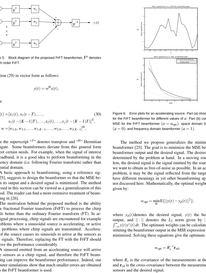
Figure 6. Error plots for an accelerating source. Part (a) shows the MSE for the FrFT beamformer for different values ofa. Part (b) compares the MSE for the FrFT beamformer(a = aopt), space domain beamformer (a = 0), and frequency domain beamformer(a = 1).
The method we propose generalizes the minimum MSE beamformer [25]. The goal is to minimize the MSE between the beamformer output and the desired signal. The desired signal is determined by the problem at hand. In a moving source prob-lem, the desired signal is the signal emitted by the source, which we want to obtain as free-of-noise as possible. In an active radar problem, it may be the signal reflected from the target. It may have different meanings in yet other beamforming applications not discussed here. Mathematically, the optimal weights woptare
given by:
wopt= minw E{||y(t) − yd(t)||2}, (31)
where yd(t)denotes the desired signal, y(t) the beamformer
output, and || · || denotes the L2 norm given by ||y(t)||2 = R∞
−∞y(t)y∗(t) dt. The optimum weights can be calculated by sub-stituting the beamformer output in the MSE expression (31) to be minimized. Solving these equations give the optimum weights:
wopt= R−1x rxd,
where Rxis the covariance of the measurements at the sensors, and rxdis the cross-covariance between the measurements at the sensors and the desired signal.
The above result corresponds to the spatial filtering of the signals arriving at the sensors. We extend this result by using filtering in a fractional Fourier domain rather than the spatial do-main. Figure shows the general structure of the proposed beam-former.
The measurements at the sensors are transformed into the ath fractional Fourier domain, then beamforming is performed in this domain, and the output is transformed back into the time domain by using the inverse FrFT. We can summarize these op-erations by writing the input-output relationship explicitly:
y(t) = F−a{wH(Fa{x(t)})}, (32)
where Fa{.} denotes the ath order FrFT. Since the structure of the beamformer is now changed we have to re-calculate the op-timum weights. The goal is again to minimize the MSE between the desired signal and the output of the beamformer. We substi-tute the beamformer output (32) into the MSE (31) to be min-imized and solve for the optimum orders. We refer the reader to [31] for details. The optimum weights that minimize the MSE are now given by:
wopt= R−1xa rxad,
where Rxa is the covariance of the ath order FrFT’s of the
sig-nals arriving at the sensors, and rxadis the cross-covariance
be-tween the ath order FrFT of the desired signal and the FrFT’s of the signals arriving at the sensors. The covariance Rxa and
the cross covariance rxadshould be known a priori in a moving
source problem. On the other hand, in an active radar problem, we can calculate it since the signal transmitted is known to us, assuming a distribution for the parameters like range, radial ve-locity and DOA of the target.
We can compute Rxa and rxadusing the original covariances
as follows: Rxa= Rxa(t,t 0) = Z ∞ −∞ Z ∞ −∞Ka(t,t 00)K−a(t0,t000)R x(t00,t000) dt00dt000, rxad= rxad(t,t 0) = Z ∞ −∞ Z ∞ −∞Ka(t,t 00)K −a(t0,t000)rxd(t00,t000) dt00dt000.
The previous discussion gives the optimum weights for beamforming in a certain fractional Fourier domain. We still need to answer the question of which domain should be selected. The optimum fractional Fourier transform order cannot be found analytically in general. Instead, we calculate the MSE we want to minimize (see equation (31)) for different a’s and select the one
that yields the smallest error. We can scan values of a ∈ [−1, 1] using a spacing as close as we wish and make fine adjustment if necessary.
The proposed method reduces to ordinary minimum MSE beamforming in the spatial domain for a = 0 and to minimum MSE beamforming in the frequency domain for a = 1. In the next section we show that in many problems the optimum order is different than 1 or 0, thus smaller errors can be obtained when the generalized method we propose is used.
We demonstrate that the proposed method yields improved results (smaller MSE) in a moving source scenario. The source is in the far field and emits an electromagnetic sinusoid with frequency f = 100 kHz, so the wavelengthλ is approximately 3 meters. We assume additive Gaussian noise and use 5 lin-early spaced passive sensors separated by half wavelength, and only instantaneous measurements are used, without delays. The source signal is assumed to be stochastic with known second-order statistics. The source accelerates from 60m/s to 120m/s during the measurement interval with an acceleration of 6m/s2
in the same direction. Figures 6 show two figures of the MSE (31) for each scenario, the first (a) as a function of the FrFT or-der a, and the second (b) as a function of SNR for beamformers in the space domain (a = 0), frequency domain (a = 1) and the proposed method for the optimum order.
Figure 6a shows that for the accelerating source the optimum order is a = 0.8, which is different than 0 and 1 (corresponding to standard space and frequency domain beamformers). The im-provements in performance can be easily observed from this plot, especially for low SNR values.
REFERENCES
[1] Ozaktas H. M., Zalevsky Z., and Kutay M. A. 2001, The Fractional Fourier Transform with Applications in Optics and Signal Processing, John Wiley & Sons.
[2] Ozaktas H. M., Kutay M. A., and Mendlovic D.,1999, In-troduction to the fractional Fourier transform and its appli-cations. In Advances in Imaging and Electron Physics 106, Academic Press, San Diego, California, 1999. Pages 239– 291.
[3] McBride A. C. and Kerr F. H., 1987, On Namias’s frac-tional Fourier transforms. IMA J Appl Math, vol. 39, pp. 159–175.
[4] Mustard D. A., 1987, The fractional Fourier transform and a new uncertainty principle. School of Mathematics Preprint AM87/14, The University of New South Wales, Kensington, Australia.
[5] Namias V., 1980, The fractional order Fourier transform and its application to quantum mechanics. J Inst Maths Ap-plics, vol. 25, pp. 241–265.
time-frequency representations. IEEE Trans Signal Pro-cessing, vol. 42, pp. 3084–3091.
[7] Lohmann A. W., 1993, Image rotation, Wigner rotation, and the fractional order Fourier transform. J Opt Soc Am A, vol. 10, pp. 2181–2186.
[8] Ozaktas H. M. and Mendlovic D., 1993, Fourier trans-forms of fractional order and their optical interpretation. Opt Commun, vol. 101, pp. 163–169.
[9] Hlawatsch F. and Boudreaux-Bartels G. F., 1992. Linear and quadratic time-frequency signal representations. IEEE Signal Processing Magazine, no:2, pp. 21–67.
[10] Bernardo L. M. and Soares O. D. D. 1994. Fractional Fourier transforms and imaging. J Opt Soc Am A, vol. 11. pp. 2622–2626.
[11] Lohmann A. W., Mendlovic D., and Zalevsky Z., 1998, Fractional transformations in optics. In Progress in Op-tics XXXVIII, Elsevier, Amsterdam, 1998. Chapter IV, pages 263–342.
[12] Ozaktas H. M. and Erden M. F., 1997, Relationships among ray optical, Gaussian beam, and fractional Fourier trans-form descriptions of first-order optical systems. Opt Com-mun, vol. 143, pp. 75–86.
[13] Ozaktas H. M. and Mendlovic D., 1995, Fractional Fourier optics. J Opt Soc Am A, vol. 12, pp. 743–751.
[14] Akay 0. and Boudreaux-Bartels G. F., 1998, Broadband in-terference excision in spread spectrum communication sys-tems via fractional Fourier transform. In Proc 32nd Asilo-mar Conf Signals, Systems, Computers, IEEE, Piscataway, New Jersey, 1998. Pages 832–837.
[15] Bastiaans M. J. and van Leest A. J., 1998, From the rect-angular to the quincunx Gabor lattice via fractional Fourier transformation. IEEE Signal Processing Lett., vol. 5, pp. 203–205.
[16] Cariolaro G., Erseghe T., Kraniauskas P., and Laurenti N., 1998, A unified framework for the fractional Fourier trans-form. IEEE Trans Signal Processing, vol. 46, pp. 3206– 3219.
[17] Kutay M. A., ¨Ozaktas¸ H., Ozaktas H. M., and Arıkan O., 1999, The fractional Fourier domain decomposition. Signal Processing, vol. 77, pp. 105–109.
[18] Mendlovic D., Zalevsky Z., and Ozaktas H. M., 1998, Applications of the fractional Fourier transform to opti-cal pattern recognition. In Optiopti-cal Pattern Recognition, Cambridge University Press, Cambridge, 1998. Chapter 4, pages 89–125.
[19] Kutay M. A., Erden M. F., Ozaktas H. M., Arıkan O., G¨ulery¨uz ¨O., and Candan, C¸ ., 1998, Space-bandwidth-efficient realizations of linear systems. Opt Lett, vol. 23, pp. 1069–1071.
[20] Yetik I. S. and Nehorai A., 2003, “Beamforming using the Fractional Fourier Transform,” to appear in IEEE Trans. on Signal Processing.
[21] Monzingo R. and Miller T., 1980, Introduction to adaptive arrays. John Wiley & Sons.
[22] Applebaum S. P. and Chapman D. J., 1976, Adaptive arrays with main beam constraints, IEEE Trans. on Antennas and Propagation, vol. 24, pp. 650–662.
[23] Capon J., 1969, High resolution frequency-wavenumber spectrum analysis, Proc. IEEE, vol. 57, pp. 1408–1418. [24] Frost III O. L., 1972, An algorithm for linearly constrained
adaptive array processing, Proc. IEEE, vol. 60, pp. 926– 935.
[25] Widrow B., Mantey P. E. and Griffiths L. J., 1967, Adaptive antenna systems, Proc. IEEE, vol. 55, pp. 2143–2159. [26] Van Veen B. D. and Buckley K. M., 1988,
Beamform-ing: A versatile approach to spatial filtering, IEEE Acoust., Speech, and Signal Processing Magazine, vol. 5, pp. 4–24. [27] Ozaktas H. M., Arıkan O., Kutay M. A., and Bozda˘gıG., 1996, Digital computation of the fractional Fourier trans-form. IEEE Trans Signal Processing, vol. 44, pp. 2141– 2150.
[28] Cohen L., 1995, Time-frequency analysis. Prentice Hall PTR.
[29] Ozaktas H. M., Barshan B., Mendlovic D., and Onural L., 1994, Convolution, filtering, and multiplexing in fractional Fourier domains and their relation to chirp and wavelet transforms. J Opt Soc Am A, vol. 11, pp. 547–559.
[30] Erden M. F., Kutay M. A. and Ozaktas H. M., 1999, Re-peated filtering in consecutive fractional Fourier domains and its application to signal restoration, IEEE Transactions on Signal Processing, vol. 47, pp. 1458–1462.
[31] Kutay M. A., Ozaktas H. M., Arıkan O., and Onural L. (1997). Optimal filtering in fractional Fourier domains. IEEE Trans Signal Processing, vol. 45, pp. 1129–1143. [32] Yetik ˙I. S¸., Ozaktas H. M., Barshan B., Onural L.,
“Perspec-tive projections in the space-frequency plane and fractional Fourier transforms,” Journal of Optical Society of America A, vol. 17, pp. 2382-2390, 2000.
[33] Candan C¸ ., Kutay M. A., and Ozaktas H. M. IEEE Trans-actions on Signal Processing, 48:1329–1337, 2000.