Forecasting stock prices by using alternative time series models: The case of Istanbul Securities Exchange

':·η_{t I . . ;}} ,·

■·,··'7·. : Til'''.

s ? a é - s

‘IBB

Μ ι ψ

FO R E C A ST IN G ST O C K PRICES B Y U SIN G

ALTE R N A TIV E TIM E SERIES M O D ELS:

The Case of Istanbul Securities Exchange

A THESIS PRESENTED BY A. OZLEM BAŞÇI

TO

THE INSTITUTE OF

ECONOMICS AND SOCIAL SCIENCES

IN PARTIAL FULFILLMENT OF THE

REQUIREMENTS

FOR THE DEGREE OF MASTER OF

ECONOMICS

BILKENT UNIVERSITY

I certify that I have read this thesis and in my opinion it is fully adeciuate, in

scope and in quality, as a thesis for the degree of Master of Economics.

Assist. Prof. Kıvılcım Metin

I certify that I have read this thesis and in my opinion it is fully adequate, in

scope and in ciuality, as a thesis for the degree of Master of Economics.

Assoc. Profy Giilnur Muradoglu

I certify that I have read this thesis and in my opinion it is fully adequate, in

scope and in quality, as a thesis for the degree of Master of Economics. .

Assist. Prof. Syed F.Mahmud

H ^

5 ^ 0 6 .Ç

ê s r

ACKNOWLEDGEMENTS

I am grateful to Assist. Prof. Kıvılcım Metin and Assoc. Prof. Gûlnur Muradoğlu

for their supervision and guidance throughout the development of the thesis. I

would like to thank Aylin Ozey from Turkish Treasury for providing the budget

deficit data.

I finally and especially would like to thank my family for their support and

ABSTRACT

The Case of Istanbul Securities Exchange

A. ÖZLEM BAŞÇI

M ASTER OF ECONOMICS

Supervisor:Assist.Prof.Kivilcim Metin

September, 1996

This study compares the forecast performance of alternative time series models at

the Istanbul Securities Exchange (ISE). Considering the emerging market character­

istics of ISE, stock prices are estimated by using money supply, inflation rate, interest

rate, exchange rate, and government deficits. First the time series properties of the

data set are examined and cointegration is tested. Next, univariate ARIM A mod­

els, V AR’s in levels and differences, and error correction models are specified and

estimated using monthly data from 1986(1) through 1995(12). According to out-

of-sample forecasting exercise it is found that the models assuming the existance of

seasonality performes poor, the more parsimonious univariate A RIM A model have

better performance than multivariate models.

Key Words: Vector Autoregression, Seasonal Unit Root, Cointegration, Error

Correction Model, Istanbul Securities Exchange, Forecasting FO R E C A STIN G ST O C K PR IC ES

oz

h i s s e s e n e d i FİYATLARININ

ÇEŞİTLİ ZAM AN SERİSİ MODELLERİYLE TAHMİNİ:

İstanbul Menkul Kıymetler Borsası Örneği

A. ÖZLEM BAŞÇI

Yüksek Lisans Tezi, İktisat Bölümü

Tez Yöneticisi: Yrd. Doç. Kıvılcım Metin

Eylül, 1996

Bu çalışma, çeşitli zaman serisi modellerinin İstanbul Menkul Kıymetler Borsasındaki

(IM KB) tahmin performansını karşılaştırmaktadır. İM KB’nin gelişmekte olan piyasa

özellikleri gözönüne alınarak, hisse senedi fiyatları; para arzı, enflasyon haddi, faiz

haddi, döviz kuru ve kamu açıkları yoluyla tahmin edilmiştir.

ilk olarak verilerin zaman serisi özellikleri incelenmiş ve ko-entegrasyon sınaması

yapılmıştır. Ardından tek değişkenli ARIM A modelleri,vektör otoregresyonları-her

değişkende hem düzey hem de değişkenlerin farkları için- ve hata düzeltme mod­

elleri belirlenmiş ve 1986(1)-1995(12) dönemini kapsayan aylık veriler kullanılarak

tahmin gerçekleştirilmiştir. Örneklem dışı tahmin uygulamasına göre, mevsimsel-

lik varsayımında bulunan modellerin performanslarının düşük olduğu, daha yalın

olan tek değişkenli ARIM A modelinin daha iyi performansa sahip olduğu bulgusuna

ulaşılmıştır.

Anahtar Kelimeler: Vektör Otoregresyonu, Mevsimsel Birim Kök, Ko-entegrasyon,

Contents

1 INTRODUCTION

1

2 THE SETTING

3

3 ECONOMETRIC THEORY

7

3.1 S ta tio n a rity ... 7 3.2 Unit Root T e s t ... 8 3.3 Cointegration A n a ly s is ... 12 3.4 Univariate ARIMA M o d e l ... 17 3.5 VAR M o d e l ...19 3.6 Error Correction M o d e l... 20

4 EMPIRICAL RESULTS

23

4.1 The Data S e t ... 23

4.2 Results of Seasonal Unit Root T e s t ... 24

4.3 Results of Cointegration Test ... 25

4.4 M o d e llin g ... 26

4.4.1 Forecast C a lib r a t io n ... 28

4.4.2 Comparison of the Different Seasonal M o d e ls...30

4.4.3 Results of the Tests for Order of the In tegration ...31

4.4.4 Comparison of Different Nonseasonal M o d e ls ...32

5 CONCLUSION

37

REFERENCES

39

APPENDIX A

44

APPENDIX A

• T able 1, T h e D a ta Set

• T able 2. R e su lts o f S eason al U n it R o o t T est

Table 2.1. Seasonal Unit Root Test of LP

Table 2.2. Seasonal Unit Root Test of LE

Table 2.3. Seasonal Unit Root Test of LISE

Table 2.4. Seasonal Unit Root Test of LR

Table 2.5 Seasonal Unit Root Test of LM l

Table 2.6. Seasonal Unit Root Test of LM2

Table 2.7. Seasonal Unit Root Test of B U T /P

• T able 3. Joh a n sen T ests fo r th e N u m b e r o f C o in te g r a tin g V e cto rs

Table 3.1. Johansen Tests for the Number of Cointegrating Vectors for the

First Data Set

Table 3.2. Johansen Tests for the Number of Cointegrating Vectors for the

Second Data Set

• T a b le 4. A D F T ests

Table 4.1. ADF Tests for 1(0)

Table 4.2. ADF Tests for 1(1)

Table 4.3. ADF Tests for 1(2)

• T a b le 5. C o r r e lo g r a m o f R esid u a ls o f A R I M A (0 ,1 ,0 )

Table 6.2. Model 2: VAR in First Difference

Table 6.3. Model 3: A

1

A

12

Filtered VAR Specification Table 6.4. Model 4: A

1

A

12

Filtered ECM Specification Table 6.5. Model 5: ARIM A(0,1,0)

Table 6.6. Model 6: VAR in Levels

Table 6.7. Model 7: VAR in Differences

Table 6.8. Model 8: ECM with Free Parameters

Table 6.9. Model 9:Two Step ECM

Table 7. Forecast Standard Errors

Table 7.1.1. Model la: V AR in Levels with 11 Seasonal Dummies

Table 7.1.2. Model lb: VAR in Levels with 11 Seasonal Dummies

Table 7.2.1. Model 2a: V AR in First Difference

Table 7.2.2. Model 2b: V AR in First Difference

Table 7.3.1. Model 3a: A

1

A

12

Filtered V AR Specification Table 7.3.2. Model 3b: A

1

A

12

Filtered V A R Specification

Table 7.4.1. Model 4a: A

1

A

12

Filtered ECM Specification Table 7.4.2. Model 4b: A

1

A

12

Filtered ECM Specification Table 7.5. Model 5: ARIM A(0,1,0)

Table 7.6.1. Model 6a: V A R in Levels

Table 7.6.2. Model 6b: V AR in Levels

Table 7.7.1. Model 7a: V AR in Differences

Table 7.8.1. Model 8a: ECM with Free Parameters

Table 7.8.2. Model 8b: ECM with Free Parameters

Table 7.9.1.Model 9a: Two Step ECM

Table 7.9.2. Model 9b:Two Step ECM

• T able 8. F orecast A c c u r a c y S ta tistics

Table 8.1. Model 1: V AR in Levels with 11 Seasonal Dummies

Table 8.2. Model 2: VAR in First Difference

Table 8.3. Model 3: A

1

A

12

Filtered VAR Specification Table 8.4. Model 4: A

1

A

12

Filtered ECM Specification Table 8.5. Model 5: ARIM A(0,1,0)

Table 8.6. Model 6: V AR in Levels

Table 8.7. Model 7: V AR in Differences

Table 8.8. Model 8: ECM with Free Parameters

Table 8.9. Model 9: Two Step ECM

APPENDIX B

• Figure 1. Graphs of ISE

• Figure 2. Graphs of P Figure 3. Graphs of E • Figure 4. Graphs of R • Figure 5. Graphs of M l Figure 6. Graphs of M2 Figure 7. Graphs of B U T /P

Figure 8. Model la: VAR in Levels with 11 Seasonal Dummies

• Figure 9. Model 2a: VAR in First Difference

• Figure 10. Model 3a: A

1

A

12

Filtered VAR Specification

• Figure 11. Model 4a: A

1

A

12

Filtered ECM Specification

Figure 12. Model 5a: ARIMA(0,1,0)

• Figure 13. Model 6a: VAR in Levels

Figure 14. Model 7a: VAR in Differences

Figure 15. Model 8a: ECM with Free Parameters

1

IN T R O D U C T IO N

Macroeconomic variables constitute a more important set of information in thin

equity markets of developing countries relative to the mature ones in industrial

countries. In thin equity markets of developing countries, the volume of trade is

low, information on company performances are limited and untimely and also cap­

ital accumulation is dominated by the state. Therefore, the thinly traded stock

markets of controlled economies are expected to absorb fiscal and monatery changes

as important sets of information.

Tests of informational efficiency with macro-economic variables conducted in ma­

ture markets report correlations between stock prices and output (Fama, 1981;

Balvers, Cosimano, McDonald, 1990), money (Pearce and Roley, 1983) and inflation

(Fama, 1990; Gultekin, 1983). More recent studies using cointegration also report

the impact of inflation (Cochran and Defina, 1993) and several money supply mea­

sures (Serletis, 1993) on stock returns.

Muradoglu and Metin (1996) provide evidence that stock prices and macro-

economic variables cointegrate at ISE and conclude that Turkish stock market is

not efficient with respect to these variables. It is known that there is an error-

correction representation which is isomorfic to cointegration. This indicates that

stock prices can be forecasted at ISE. Since more than one cointegrating vector was

obtained, the variables of concern were also used in a short run dynamic structural

model which also provided evidence that the Turkish stock market assimilates this

information with a lag.

forecasting stock returns at ISE. Considering the emerging market characteristics of

ISE as well as the results of previous research concerning the inefficiencies in this

market (Muradoglu and Metin, 1996) forecast models are based on a set of real,

financial and nominal variables.

First issue to be discussed is the forecast performance of the different seasonal

time series model at ISE. We try to see whether modelling the seasonality improve

the forecast accuracy. Another issue is that whether using the multivariate time se­

ries models improve forecast accuracy and provide an advantage over the univariate

models (A RIM A ).

Accordingly, the rest of the study is organized as follows. In Chapter 2 we present

the main features and developments of Turkish economy for the period 1986-1995.

In Chapter 3, the econometric theory used in this study is explained. In Chapter

4, we first analyze the time series properties of the data set by testing seasonal unit

roots and cointegration. According to the information revealed by these test, we

set up the specificatians of the models including seasonality. Second we set up the

results of the unit root tests. According to the results of the unit root tests forecast

models without seasonality are estimated. Finally in Chapter 5, concluding remarks

are made regarding the forecast performances of respective models. The tables and

2

TH E SETTIN G

From the beginnig of 1980 onwards, Turkey embarked on a structural adjustment

programme based on market economy principles, which includes modernizing finan­

cial markets and liberalizing capital movements. The announced policies in the

beginning of 1980 by the Turkish government included convertibihty of the Turkish

lira, switch from fixed to flexible exchange rates regimes and some export promotion

measures.

Compared with the first half of the 1980s, the period from 1984 has been charac­

terised by less stable macroeconomic performance. The Central Bank targeted some

monetary aggregates in 1986 for the first time ever. In 1986, M2 grew 38.6% which

was close to the target. The targeting exercise was continued in 1987 and 1988, but

the targets were exceeded in both years by a substantial amount. The consumer

price inflation was 35% on average for 1986 and 1987 but it reached 75.4% in 1988.

Another property of the 1986 was that the stock market became operational with

the establishment of Istanbul Securities Exchange (ISE) in the early period of the

year although the legal framework for a securities exchange had been completed in

1982. In the beginning, 42 companies were listed and today there are more than

200 stocks acting in the ISE.

Real effective exchange rate appreciation is seen from the fourth quarter of 1988

to beginning o f 1990. The real appreciation is related to the combined effect of a

high nominal interest rate differential between Turkey and the rest of the world and

inflows.

In August 1989 Decree .32 is adopted. It introduce a package of liberalization mea­

sures and freeing operations by residents and non-residents in securities investment,

easing restrictions on operations in commercial and financial credits, and permit­

ting transfer related to block funds and certain real-estate activities. In April 1990,

Turkey accepted the obligations of Article 8 of the International Monetary Fund

Agreement. Thus, Turkey has undertaken to assure the convertibility of Turkish

lira and to refrain from imposing restrictions on payments and transfers for current

international transactions.

The Central Bank did not undertake a monetary programme for 1989. In Jan­

uary 1990, the Central Bank announced a new monetary programme which consist

principally of controlling the volume of its own balance sheet, both on the asset and

liabilities side.

Hit by the events in the Gulf crisis, economic expansion came to halt by the

end of 1990. Real GNP have fallen to 1.5 per cent in 1991. Inflation continued to

worsen in 1991, along with a sharp increase in the public sector borrowing require­

ment (PSBR) 10.5 % of GDP in 1990, the highest in a decade. This was largely

due to the doubling of the State Economic Enterprises’s (SEEs) borrowing need to

5.3 per cent of GNP. In order to support Turkish lira exchange rate and to prevent

inflationary spill-overs, money market interest rates increased exteremly in the late

The volume of trade in ISE has made sharp increases in 1990 and 1993. In 1990

it increased from 751.6 to 5226.1 million dollar and in 1993 from 8378.2 to 21278.1

million dollar.

There were no fundamental change in the public sector financial position in 1992-

1993. PSBR is estimated as 12.6 percent of GNP in 1992. Inflation has reached an

average of 68.2% in the period 1988-1992 where M l, M2 and reserve money growth

was 62.5%, 67%, and 58% on the average. In 1993 PSBR rose to 16% of GNP.

Annual consumer price inflation averaged 66% in 1993. At the end of 1993, interna­

tional creditworthiness was downrated and the Turkish lira drastically depreciated

because of the high output growth in 1992 and 1993, foreign indeptedness, inflation­

ary pressures and trade deficits.

Starting in 1994, Turkish economy have undergone the most important crisis of

the last 15 years. A progressive increase occured in the PSBR from some 3.5 percent

of GDP in 1986 to over 12 percent in 1993. Further higher interest rates of inflation

led to increasing foreign currency substitution for the Turkish lira. From 1990 to

1992 the overriding goal of the Central Bank was to restore control of its own balance

sheet. To achieve this goal a monetary programme was announced.lt targeted the

key balance-sheet components such as Central Bank money, total domestic assets,

and total domestic liabilities. Combined with lax fiscal policy, the result was high

real interest rates and an appreciating real exchange rate.

On April 1994, a stabilization programme was launched to halve the ratio of the

forms. By December 1994, noteworthy progress had been made in cutting public

sector borrowing requriement and bringing the current account into surplus.

An increase in imports led to a widening of the current account deficit from 0.6

percent of GDP in 1992 to 3.9 percent of GDP in 1993. A major success of the

April 1994 programme has been the rapid restoration of external balance. A large

part of the improvement in the current account reflected the sharp drop in the real

eifective exchange must also have contributed to the swing. But average Consumer

price inflation reached to 106% where real GNP growth was -6%.

Custom union was implemented on January 1. The custom union is likely to

present a major competitive challenge to some sectors of Turkish industry. The

economy grew by 7.1% in 1995. The growth in M l and M2 was 71% and 102% re­

spectively. The monthly rises in the CPI slowed during the fourth quarter. Annual

consumer price inflation was 95.3% and wholesale price inflation was 88.6% . The

nominal appreciation of the dollar against the lira for 1995 was 51% means that the

dollar had depreciated against the lira in real terms. The volume of trade in ISE

reached to 52358 millón dollar in 1995.

Above developments in Turkish economy causes Turkey to be a good case study

as a developing country. In this study we try to forecast Turkish stock market by

3

E C O N O M E T R IC T H E O R Y

3.1 Stationarity

A stochastic process is said to be stationary, if the joint and conditional distribution of the process is unchanged if displaced in time.

For an arbitrary stochastic process A'(t), i G T the distibution function F{X{t))·, 0<) depends on t with the parameters 0 ( characterising it being the functions of t as well.

A stochastic process X { t ) , t G T is said to be (strictly) stationary if for any subset {ti, t2, .■■,tn) of T and any r,

F { X { h ) , ...,X{tn)) = F { X { U + r ) , ..., X { U + r ))

which means,the distribution function of the process remains unchanged when

shifted in time by an arbitrary value r. In terms of the marginal distributions

F { X{ t ) ) , t G T stationarity implies that

F ( X { t ) ) ^ F ( X ( t + T ) ) ,

and hence F{ X{ t i ) ) = F { X { t2) = ··· = F{ X{ tn) ) (Spanos, 1986).

A stocastic process Xt is said to be stationary in a weak sense if:

E{Xt) = constant = f.1 ; Var[Xt) = constant = cr^

and:

Thus the means and the variances are constant over time and the covariance

between two periods depends only on the gap between the periods, and not the

actual time at which the covariance is considered. An autoregressive model as given

below ,

y t = a + 0 y t - i + Ci

where Cj denote a series of identically, independently distributed continuous ran­

dom variables with zero means.

is stationary if \/3\ < 1.

Most economic time series are not stationary. It has been shown in a number

of theoretical works that, in general, the statistical properties of regression analysis

using nonstationary time series are dubious. However, many of them can at least

be approximated by stationary process if they are differenced. If a series must be

differenced d times to make stationary, it is said to be integrated o f order d . This is expressed by writing yt ~ /(d ).

3.2

Unit Root Test

Before any sensible regression analysis can be performed, it is essential to identify

the order of integration of each variable. An appropriate method of testing the order

of integration has been proposed by Dickey and Fuller (1979), which is called DF

test. For an first order autoregressive equation:

the DF test is a test of the hypothesis that p = 1, so it is a unit root test. This

test is based on the estimation of an equivalent regression equation to (1), namely:

^Vt — ^Vt-i + (-t (2) Equation can be re-written as:

J/t — (1 + ^)yt-i +

which is the same as (1) with p = (1 + 6). The Dickey-Fuller test consist of testing the negativity of 8 in the ordinary least squares regression of (2) where the null {Ho)

and alternative (Hi) hypothesis are:

Ho·. 6 = 0

H i: 8 < 0

The rejection of the null hypothesis implies that the process is integrated of or­

der zero. To evaluate the hypothesis, we use the critical values tabulated in Fuller

(1976), because student t-ratio does not have a limiting normal distribution because

of the unit root.

If we reject the null hypothesis, we conclude that yt is 1(0). But if the null can not be rejected, the next step would be to test whether the order of integration is

one. The Dickey-Fuller equation is now:

AAyt =

8Ayt-i

_{+ e<}

this process goes on by differencing yt each time until we become able to reject the null hypothesis.

A weakness of the original Dickey-Fuller test is that it does not take account of

possible autocorrelation in the error process. If tt is autocorrelated, then the ordi­ nary least squares estimates of equation (2) is not efficient. A solution advocated

by Dickey and Fuller (1981), is to use lagged left-hand side variables as additional

explanatory variables to approximate the autocorrelation. This test, called the Aug­ mented Dickey-Fuller test, and denoted conventionally as A DF , is widely regarded as being the most efficient test from among the simple tests for integration and is

in present the most widely used in practice.

The ADF equivalent of (2) is the following :

k

Ayt = Syt-i -h ^ 6iAyt-i -f tt i=l

To specify the lag length k there are several criteria. A maximum lag length is

specified first then the equation is estimated with k = l,2 , ....,kmax· According to final prediction error (FPE) criterion for each estimation the one with smallest FPE is selected. Akaike information criterion AIC suggest to select the equation which has the minimal loss of informât ion,i.e, the smallest AIC. In an alternative way first,

the regression is estimated with maximum lag length. If the last included lag is

significant, the maximum lag length is is specified as appropriate lag length. If not,

than the number of lags is reduced one by one until the coefficient on the last lag is

significant (Ng and Perron, 1993).

Testing For Seasonal Unit Roots

A nonstationary series is said to be seasonally integrated of order (d,D), denoted 5/a(d, £>), if it can be transformed to a stationary series by applying s-differences

D times and then differencing the resulting series d times using first differences. A

method has been developed for testing for seasonal unit roots proposed by Hylleberg

et al.(1990) for quarterly data and by Franses (1991) for monthly data.

In the case for monthly data, the presence of 12 roots on the unit circle can be

seen from the decomposition of the differencing operator A

12

: l - B ' 2 ^ ( l - B ) ( l + 5 ) ( l - i B ) ( l + iB )

[1 + (^/3 + i)B/2][l + ( V3 - i)B/2]

[1 - (v/3 + i)B/2][l - { V s - i)B/2]

[1 + (v/3 + 1)B/2][1 - { V s - l)B/2]

[1 - (V 3 + l)B/2][l + { V S - 1 )5 /2 ]

where (1-B) corresponds to unit root, the remaining terms represent seasonal unit

roots.Testing for unit roots in the monthly time series data requires to test the

significance of the coefficients of the following auxiliary regression given below;

¥’* ( 5 )j/ 8,< = 7 T iy i,t_ i + 7r2j/2,<-2 + 7r3?/3_(_i

+ 7T 4i/3,i-2 + T ^ s y 4 , t - 1 + 7r6j/4,t-2

+ 7 T 7 j/5 ,t-l + ^ 8 i/5 ,i-2 + TTgye.t-l

+ ’ Tl0i/6,t-2 + 7T nJ/7,i_i + 7Tl2i/7,i-2

+ f i + Ci

where (p is some polynomial function of B and pt covers the deterministic part, and where

!/i,, = (1 + B )(l + B* + B > , J/2,t = —(1 — B ) ( l + j/

3

,t = - { 1 - B ^ ) { l + B^ + B^)yt

=

- { I - - V3B + B'^){1 + B^ + B^)yt ys,t = - i l - B ^ ) { l + VSB + B^){l + B^ + B^)yt ye,t = - { I - B^)(l - B^ + B^)(l - B + B^)yt yj,t = - { 1 - B^)(l - B^ + B^){1 + B + B^)yt ys,t = { l - B^ ^ ) y t

Testing for (seasonal) unit roots requires estimation of tt’s first by using ordinary

least squares and the testing the statistical significance of tt’s second. Since the pairs

of complex unit roots are conjugates, these roots only appear when pairs of tt’s are

jointly equal to zero. If tti = 0, then the presence of root 1 can not be rejected.

There will be no seasonal unit root if, tt2 through 7Ti2 are significantly different

from zero. When tti = 0, 7T2 = ... = 7Ti2 ^ 0 then seasonality can be modelled by

using elevan seasonal dummies. In case all x,·, i=1...12, are equal zero, filtering

requires to eliminate some seasonal unit roots (Franses, 1991).

3.3

Cointegration Analysis

If there is a long run relationship between two (or more) nonstationary variables, the

deviations from this long run path are stationary. If this is the case, the variables in

question are said to be cointegrated. The formal definition of cointegration of two variables, developed by Engle and Granger (1987) is as follows:

Time series Xt and yt are said to be cointegrated of order d,b where d > b > 0,

written as :

xt,yt ~ CI{d, b),

if:

1- both series are integrated of order d,

2- there exists a linear combination of these variables,say aio:t + a

2

j/t,which is integrated of order d-b .

The vector [ «

1

,

02

] is called a cointegrating vector.

More generally:

If Xt denotes an n x 1 vector and each of series in Xt are 1(d) and there exists an n X 1 vector a such that x[a ~ I{d — 6), then x'tQ ~ CI{d,b).

For empirical econometrics, the most interesting case is where the series trans­

formed with the use of the cointegrating vector become stationary, that is where

d = b, and the cointegrating coefficients can be identified with parameters in the long run relationship between the variables.

We use the Engle-Granger Two-step approach in estimating the linear combina­ tion of variables which is integrated of zero.

Consider the long run relationship:

yt = ^xt + ut (3)

grating vector is known a priori the residuals are calculated from that known long

run equation. Then we test whether the residual Ut is 1(0) or not when the series are integrated of the same order. To test this, the equation given below is used;

Arit — ^Ut-i + ^ ^ ¿j·Ai_,· + tt

(=1

which is the Augmented Dickey-Fuller equation. Again the null hypothesis is

is not 1(0) which implies Xt and t/j are not cointegrated. So if the null hypothesis is rejected we conclude that X( and yt are cointegrated.DF equation also can be used for cointegration test. The critical values for ADF cointegration test are given in

Engle and Granger(1987). Engle and Yoo (1987), extend the test for cointegration

according to Engle and Granger for different sample sizes and numbers of variables.

Multivariate Cointegration:

The second test employed for cointegration analysis is the maximum likelihood procedure suggested by Johansen (1988). This procedure analyses multicointegra­ tion directly investigating cointegration in the vector autoregression, VAR, model.

Consider the unrestricted VAR model:

Zt — y ] AiZt-i -b Ct

¿=1

where Zt contains all n variables of the model and Ct is a vector of random errors.

We will assume throughout that all the variables in Zt are integrated of the same order, and that this order of integration is either zero or one. The VAR model can

be represented , ignoring the deterministic part (intercepts, deterministic trends,

seasonals, etc.) in the form:

A:-l

^ Z t — ^ ^ r,A Z i_ , + WZt-k + t= l

where:

r,· = —I + A i + ... + Ai ( / is a unit matrix)

U = - { I - A , - . . . - A k )

Since there are n variables which constitute the vector Zt the dimension of II is

n X n and its rank can be at most equal to n. If the rank of matrix II is equal to r < n, there exists a representation of II such that:

n = a/3\

where a and ^ are both n x r matrices.

Matrix ^ is called the cointegrating matrix and has the property that ^'Zt m ,

while Zt ~ -1(1)· The columns of ¡3 contain the coefficients in the r cointegrating vec­ tors.

The procedure followed for the determination of r is :

By regressing AZt and Zt-k on A Z t_i, A Z t_

2

, ..., AZ(_fc+iwe obtain residuals Rot

and Rkt- The residual product moment matrices are,

T

Sij = T~^ RitR'jt, i^j = 0, k [T = samplesize) t=i

Solving the eigenvalue problem,

\flSkk SkoSao iSoA:| = 0,

yields the eigenvalues /ii > fi2 > ... > fin (ordered from the largest to the smallest) and associated eigenvectors u,· which may be arranged to the matrix

V = [i)i,

1

)

2

, The eigenvectors normalized such that V'SkkV = I- If the cointegrating matrix /3 is of rank r < n ,the first r eigenvectors are the cointegrating vectors, that is they are the columns of matrix /3. Using the above eigenvalues, the null hypothesis that there are at most r cointegrating vectors can be tested by

calculating the loglikelihood ratio test statistics:

n

LR = - T

ln(l-fii),

t= r+ l

which is called as the trace statistic (Johanses and Juselius 1990). Normally test­ ing starts from r=0 , that is from the hypothesis that there are no cointegrating

vectors in a VAR model. If this can not be rejected the procedure stops. If it is

rejected, it is possible to examine sequentially the hypothesis that r < l , r < 2, and

so on.

There is also a likelihood ratio test known as the maximum eigenvalue test in which the null hypothesis of r cointegrated vectors is tested against the alternative

of r-1-1 cointegrating vectors. The corresponding test statistic is:

LR = —Tln{l — fir),

The critical values of these tests are tabulated in Johansen and Juselius (1990)

Now we will examine the methodology of alternative time series models; uni­

variate ARIM A model, vector autoregression in levels and differences, and error

correction model.

3.4

Univariate A R I M A M odel

If a process y can be represented in the form:

J/f = «0 + OiJ/i_i -|- ... -|- Opt/i-p tf\ - -f- ... -|- Pqtt-q (4)

where €t is a white-noise process, which means each value in the sequence has a mean of zero, a constant variance and is serially uncorrelated.If the characteristic

roots of (4) are all in the unit circle,{j/t} then is called an autoregressive moving

average model of orders p and q (A R M A (p,q)) for yt (Enders, W .(1995)). If p = 0 then the process is called a moving average process of order q (M A (q)) and if q= 0

the process is called an autoregressive process of order p (A R (p )). If both p and

q are zero, then the process is white noise. However, if one or more characteris­

tic roots of (4) is greater than or equal to unity, the {pt} sequence is said to be

an integrated process and (4) is called an autoregressive integrated moving average

(ARIM A) model (Box and Jenkins (1976)).

The attraction of the A RM A (p,q) model is that it provides a parsimonious rep­

resentation of a stationary stochastic process. It may be extended to encompass a

much wider class of non-stationary models by differencing. If the difference oper­

ator must be applied d times before an A R M A (p,q) representation is appropriate

(integration is performed d times), the variable is said to follow an autoregressive

One natural question to ask of any estimated model is: How well does it fit the

data? Adding additional lags for p and/or q will necessarily reduce the sum of

squares of the estimated residuals. But the inclusion of extraneous coefficients will

reduce the forecasting performance of the fitted model.

The basic tool for specifying suitable values of p and q is the correlogram is

also called the autocorrelation function (ACF) and partial autocorrelation function

(PACF). If the sample is reasonably large ACF and PACF should display a similar

pattern to that of the underlying theoretical autocorrelation function. A knowledge

of the patterns of ACF and PACF’s typically associated with different values of p

and q can lead the researcher to make an appropriate choice.

After estimating the chosen model, its adequecy can be assesed by testing whether

the residuals are approximately random. The main test statistic used is the Box- Pierce Q-statistic, which is defined as

Q = T ± r l i = l

where rt is the t’th sample autocorrelation in the residuals. If the model is cor­ rectly specified, Q has a distribution with P — p — q degrees of freedom. High values of Q lead to a rejection of the hypothesis o f correct specification. If the model

3.5

V A R Model

Vector auto regressions (VARs) provide a valid representation for forecasting of sys­ tem of economic time series (see Sims (1980) and Litterman (1986))). General vector

autoregressive model consist in regressing each current (non-lagged) variable in the

model on all the variables in the model lagged a certain number of times.

One straightforward application of an unrestricting VAR model is for forecasting.

A VAR forecaster does not worry about the economic theory underlying VAR model

and, more importantly, does not need to make any assumptions about the values of

exogenous variables in the forecasting period.

Consider, the simple bivariate system:

Vt = <^10 + Oiij/i-i + Oi22t_i + eit

Zt — 0-20 + 0 ,2 i y t - l + 0,22^ t-\ + ^2t

where it is assumed that both j/jand Zt are stationary; eu and t2t may be corre­ lated. These equations constitute a first order V AR since the longest lag length is

unity. We may also have VAR in differences,a V A R in first difference has the form:

A x t = 7To -I- 7Ti A x t - I + 7 T 2 A x t_2 -b ... + T T p A x t-p -t- Ct

where

Xt — (2:11, X 2ij ···? ^ n i)

TTo = (n X l)vector of intercept terms with elements 7t,o

7T,· = (n X n)coefficient matrices with elements 7Tjjt(z) i — l...t — p Ct = an {n X l)vector with elements e,i

The disturbance terms t'^s are white-noise where tn may be correlated with ejt·

3.6

Error Correction M odel

Formally, the (n x 1) vector Xt = {x\uX2ti has an error-correction represen­ tation ^ if it can be expressed in the form:

AXi = TTO + TTXi-i -I- 7TiAXi_i -I- 7T2AXi_2 -|- ... + TTpAxt-p d- Ct (5)

where

7To = an (n X 1) vector of intercept terms with elements tt.o

7T, = (n X n) coefficient matrices with elements TVjkii) i = l . . . t — p

7T = is a matrix with elements TTjk such that one or more of the TTjk / 0

= an (n X 1) vectorwith elements e,(

The disturbence terms e,i‘ s are white noise and may be correlated with Cjt

Let all variables in Xt be /(1 ). Now if there is an error-correction representation of these variables as in (5), there is necessarily a linear combination of the 1(1)

variables that is stationary. Solving (5) for Trxt-i yields;

T T X t - i = A X i — 7To — ^ 7T,· A x t _ i — 6 t

Since each expression on the right-hand side is stationary, 7rXf_i must also be

tionary. Since tt contains only constants, each row of tt is a cointegrating vector of

Xt. For example, the first row can be written as (7rnarii_i + 'X\2X‘2t-\ + ···+ 7Ti„Xni-i)· Since each series Xu-\ is /(1 ), (tth, 7Ti2, must be a cointegrating vector for Xf

If all elements of tt equal zero, (5) is a traditional VAR in first differences. In

such circumstances, there is no error-correction representation since Axt does not

respond to the previous period’s deviation from long-run equilibrium.

Since ECM embodies both short-run dynamics and the long-run constraint, it

can be used to produce optimal forecasts. In Engle and Yoo (1987) there is a more

formal representation:

Let X( be an iV X 1 vector of 1(1) series, so that:

(1 - B)xt = C {B)et

where B is lag operator and C (B) is a matrix of polynomials in B.

is a vector white noise process with

E {tt) = 0, Vf > 1

where i) is an AT x JV positive definite matrix and 6 is the delta function. The rank of C (l) is less than N.

According to Granger representation theorem (Granger, 1983) if Xt satisfies the assumptions given above, then there exist an error correction representation with

4

E M PIR IC AL RESULTS

The first part of this chapter provides the definition of the data set, the variables

used in analysis and the source of the data. Then the empirical results of testing

stationarity and cointegration will be presented. Finally in the modelling subsection

the implementation of the models and the forecast performances of the alternative

models will be examined.

4.1

The Data Set

The data set consists of monthly observations for the variable of interest between the

period of 1986:1-1995:12. Considering the macroeconomics of the Turkish economy,

we have set the relations between stock returns and a set of macroeconomic variables.

Stock returns (ISE) are represented by the monthly composite index value of the

Istanbul Securities Exchange. Considering the relationship between inflation and

the budget deficit (Metin, 1994, 1995) budget deficit is included in the data set.

Budget deficit (B U T /P ) is represented by the real budget balance (nominal budget

balance over consumer price index). Interest rates (R) are depicted by the monthly

compounded value of the annual treasury bill rate which is a sensitive measure of the

” going rate of interest” in the financial media. The Turkish lira-U.S. dollar exchange

rate (E) is included due to the frequent market operations of the Central Bank using

dollar reserves. Inflation (P ) is represented by the consumer price index. Finally,

money supply is represented by two monetary aggregates; M l which is currency

in circulation plus demand deposits and, M2 which is M l plus time deposits. All

data are collected from several issues of the Three Monthly Bulletin of the Turkish

4.2

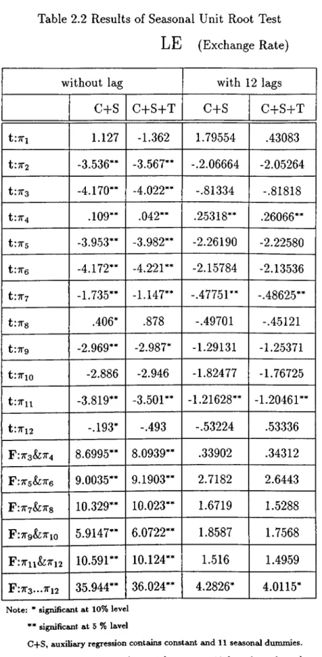
Results of Seasonal Unit Root Test

The seasonal unit root test is applied according to Franses (1991) as discussed in

subsection 3.2.The results are presented in Table-2.1 through Table-2.7. We have 4

auxiliary regressions. First and third one includes constant and seasonal dummies,

second and fourth one includes constant, seasonal dummies and trend. In the first

and second one there are no lags of dependent variable, while in third and fourth one

there are 12 lags of the dependent variable. All the series are in log form, denoted

by L, except real budget balance.

The t statistic on ttI is indicative of a strong unit root at the nonseasonal fre­

quency for all series although the evidence for LISE is not overwhelming. So all the

variables are non-stationary. There is also strong evidence that nonseasonality is

accepted for LISE.

The first and second regression results show that nonseasonality is definitly ac­

cepted for LE (except for ttIO for the first and second regression and ttS, 7t12 for the

second regression). This result is not so clear according to third and fourth regres­

sion, although nonseasonality is accepted for through 7t3 to 7t12 at 10% significant

level. LE is not seasonally integrated.

According to first and second regression results nonseasonality is accepted for LP

(except for 7t4, 7t7, 7t8 and

7

t

12

for the first and second regressions). According to third and fourth regression it is not so obvious although nonseasonality is accepted

For LMl and LM2 the results seem similar. For the first and second regression

nonseasonality is accepted (except for ttS, tt8 and 7t12 for M l and 7t4, ttS, ttS for M2). But nonseasonality is accepted for through ttS to 7t12 only in fourth regression

and at 10% level. LM l and LM2 are most probably not seasonally integrated.

For the B U T /P the result is inconclusive, since third and fourth regression results

accept seasonal roots (except for ttT at 10% level). But first and second regression

results rejects for many roots and also for through 7t3 to 7t12.

Same argument is valid for LR. The third and fourth model accept seasonal roots

(except for ttII). But first and second model rejects for many roots and also for

through 7t3 to 7Tİ2.

4.3

Results of Cointegration Test

In order to test for cointegration the maximum likelihood procedure developed in

Johansen (1988) and Johansen and Juselius (1990) is used. Test statistics are re­

ported in Table-3.1 and Table-3.2. There are two information set available, the one

consists of ISE, R, E, P, B U T /P , M l and the other ISE, R, E, P, B U T /P , M2. The

results for each information set are reported. Looking at both the trace and the

maximum eigenvalue statistics results lead us to accept definitely one and possi­

bly two cointegrating relationship for both of the tests. From the first row of the

standardized eigenvectors.

L ISE = -O .S m L E - 5.236LR -b 1.392LM1 - O .m Z B U T lP + 3.226TP - 0.1173

LISE = -0.0875LE - Q.2 2 0LR - 3.369LM2 - O .im B U T / P + 8.265LP - 0.15

The standardized loadings for both model show that the main effect of the coin­

tegrating vector is on (LISE), however there is almost no effect on the others. This

is a strong indication of the weak exogeneity of these variables for the long-run

parameters of the stock returns.

4.4

Modelling

Using the general class of ARIM A and VAR models we formulate our models. A c­

cording to two information sets, the models are reported as ’’ model a” and ’’ model

b” , respectively.

For nonstationary variables which are cointegrated the usage of the first differ­

enced variables in the VAR model is incorrect. The Granger representation theorem

implies that the cointegrated variables are related through an error correction model

(ECM) which includes the differenced variables and also the levels of the cointe­

grated variables. Therefore just using differenced variables omits the information of

the long run revealed by the levels of the variables and will, in general lead to poor

forecasts (Holden, 1995). So we also formulate error correction models.

At the first step the four seasonal models are compared through application of

stochastic and deterministic seasonality. One of them is the multiplicative seasonal

model developed by Box and Jenkins (1976) which requires that the variable is

A iA i2j/i — et + ß i e t - i + ^2^-12 + ß s ^ t-is

where

A fct/t = (1 - B ' ^ ) y t = y t - y t - k

and where tt is assumed to be a white noise process with zero mean, constant variance and E{ttes) = 0 for i s

Transforming a series with A

1

A

12

filter assumes the presence of 13 roots on the unit circle, two of which are at zero frequency. Therefore in case of non-seasonal

root only (T B ) filter is appropriate to remove non-seasonality.

The other one is the autoregressive moving average model for the variable yt in first differences in which a constant and 11 seasonal dummy variables.

11

#p(5)Aiyi — ao -h

otiDit

+

Q q [ B ) e t

i= l

where Du represent 11 seasonal dummies. The ^p{B) and 0 ,( B ) are polynomials in the backward shift operator B (Granger and Newbold 1986).

At the second step we compare four different nonseasonal models and univariate

ARIM A model. But first the order of integration of each variables is specified by

using the ADF tests.

The forecast performance of each variables are compared using several calibrations

4.4.1 Forecast Calibration

The model is estimated using less 1, 3, 6, 9, 12 forecasts. The type of forecast have

been made here, is one step ahead forecasts conditional on the observed values of

lagged variables. This is done under the assumption that one making a forecast for

period t+1 knows the realized values of the variable of interest in t.

Parameter constancy forecast tests:

Under the null of no parameter change, three parameter constancy tests are based

on the following approximate test statistics over a forecast horizon of H period: The

statistics compares within and post-sample residual variances. The null hypoth­

esis is of no parameter change in any parameter between the sample and the forecast

periods. The F equivalents of each tests are expected to have better small sample

properties.

Three types of parameter constancy tests are reported, in each case as a A'^(nH)

for n equations and H forecasts and a F(nH, T-k) statistic:

(a) using

This is an index of parameter constancy, ignoring both parameter uncertainty

and intercorrelation between forecast errors at different time periods.

(b) using V[e]

This test is similar to (a), but takes parameter uncertainty into account.

(c) using V[E]

Here, V[E] is the full variance matrix of all forecast errors E, which takes both

The forecast performance of the models at each horizon is subsequently evaluated

using three measures of errors, forecast standard errors (FSEs) means of forecast er­ rors (MFEs), and standard deviations of forecast errors (DFEs), where MFEs and DFEs show the forecast error accuracy.

The 1-step forecast errors (from T-1-1 to T + H ) are defined as:

er+j = 2/T+i — niyr+i' = (n — n)u;r+,· + ur+t

FSE is calculated from the estimated variance:

V[eT+i]

—

ii(l + Wy^,(VF'VF)“ ^iU7’4.,·) = 'ir+j

FSE provides confidence intervals for the forecasts, or a range within which fore­

cast values would be expected to lie, if the model is performing in the post sample

period as it has in the sample period.

MFEs show the average bias for all variables, which are with DFEs reported and

together imply forecast accuracy. For a model high bias and high forecast error

deviations indicate poor forecast accuracy. If the forecast period is short, MFE

and DFE results are not safe to make any comparison, since they consist of the

calculation of a few numbers. In order to make more meaningful comparisons 1 and

4.4.2 Comparison of the Different Seasonal Models

Results of the seasonal unit root tests implies that there is no stochastic seasonality

for most of the variables. So in the first step we compare the performance of the

four seasonal multivariate models, which include both stochastic and deterministic

seasonality.

Lag lengths were choosen according to Schwarz criterion which is calculated as:

SC = loga^ + k{logT)/T

So lag lengths are specified as one.

Due to April 1994 crisis there is a structural break in exchange rate, interest rate

and consumer price index. We put a step dummy from 1994(4) to 1995(12) to each

model in order to solve the structural break problem.

The first specification is a VAR model with a deterministic component; constant, trend and 11 seasonal dummies. The second model is specified as a first difference VAR with constant and 11 seasonal dummies. In the third specification we apply AiAi

2

filter to the closed V AR and a constant is included. In this specification stochastic seasonality is considered. Our last specification in this subsection is a monthly seasonal ECM representation of A

1

A

12

filter in which an ECM term is defined as L IS E t-12, L E t-u , L R t-12·, LPt-12·, L M t-12, BUT/Pt-1 2 and also constant is included. ECM reveals both short-run and long-run influences of the stochastic

seasonality of the data on different forecast horizons.

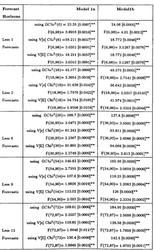
the specifications parameter constancy is rejected except for A

1

A

12

filtered ECM with the first data set (model 4a), in the very short horizons (1 and 3 months).

FSEs are reported in Table-7.1.1 through Table-7.4.2. According to the FSEs

comparisons of ISE between the models, VAR in levels with 11 seasonal dummies

(model 1) and VAR in first difference (model 2) have similar FSEs ; A

1

A

12

filter filtered VAR (model 3) and ECM (model4) have higher FSEs, where ECM has the

highest FSE.

MFEs and DFEs also confirms these results (Table-8.1 through Table-8.4). While

MFEs which shows the average bias for the variables, is smaller only for model 3 in

less 6 and less 12 forecasts and for model 4 in less 9 forecasts, the high DFE’s for all

cases indicates higher mean square forecast errors (MSFEs), since MSFE combines the squared bias in forecast errors with the forecast error variance, which is equal to

MFE^ 4- DFE^. Again VAR in levels (model 1) and V AR in first difference (model 2) have similar MSFE.

The weak performance of the stochastic models also support that there is no

stochastic seasonality in the data set. So we conclude that specification of nonsea-

sonal models is also required. Therefore we test the order of integrations of each

variables first to model the data accordingly.

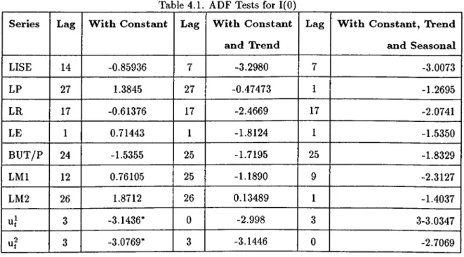
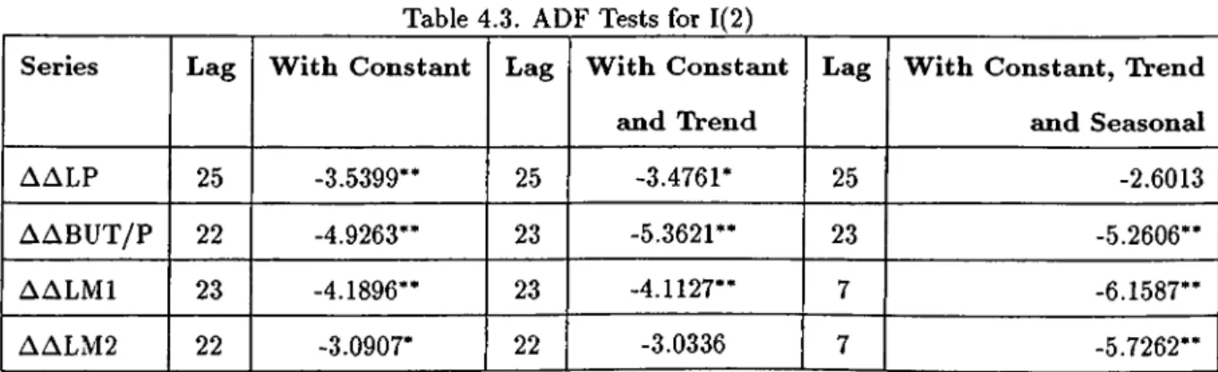
4.4.3 Results of the Tests for Order of the Integration

In order to test for the order of integration of the variables ADF test is used as dis­

cussed in the subsection 3.2. The results of the ADF tests are presented in Table-4.1

The different ADF values with including constant, constant and trend and con­

stant,trend and 11 seasonal dummies are reported. The ADF test results with

constant is considered for a baseline modelling. The other values are tabulated as

further information for the readers.

In order to specify the lag length general to specific method is used (Ng and

Perron (1995)). We begin from 30 lags. The last significant lag is specified as the

lag length and the related ADF values are reported.

All the variables are not 1(0) in 1% significance level, while the first differenced

series of LISE, LE do not exhibit a unit root at 1% and LR at 5% level. The second

differences of LP, BU T/P, LM l do not exhibit a unit root at 1% and LM2 at 5% level.

So, according to ADF test results we conclude that LISE, LE, LR are 1(1), and

LM l, LM2, B U T /P are 1(2). The graphs of the series are presented in Figure 1

through 7. The nonstationarity of each series and different order of integration of

each series can also be observed from the graphs.

4.4.4 Comparison of Different Nonseasonal Models

Five models are formulated according to the order of integration of each series in

this subsection. These models do not include any seasonal dummy or seasonal dif­

ferencing.

The first one is univariate ARIM A model. Identification of the univariate model

first differece is modelled. The correlogram of residuals indicate that a random

walk with a drift model is appropriate for ALISE (Table-5). None of the individual

autocorrelations, and partial autocorrelations of the residuals from this model are

large, and the Q-statistics -discussed in subsection 3.4 - of the residuals indicate

that they are not significantly different from zero. So Q-statistics confirm that these

residuals are white noise. The drift parameter is also significant. These are strong

evidences that the ARIMA(0,1,0) model fits the data well. So, the fifth model is an ARIM A (0,1,0).

(1 - B )L IS E = 0.050354 + m

for the period 1986:2-1995:12.

Dropping the step dummy and 11 seasonal dummies decreases the forecast errors,

so we do not used any dummy in the models. The lag length for the new models is

specified again as one (see subsection 4.4.2).

The sixth model is VAR in levels with a constant. The seventh model is VAR in differences with constant. All the variables in the model differenced so that each of

them becomes stationary. So the model consist of the first difference of LISE, LE

and LR; second difference of LP, LM and B U T /P .

There are two types of approach for error correction modelling. In the first ap­

proach xt-\ is entered separately in the V AR in a difference model, without imposing the restriction that the error correction term be identical in each equation as in model

4 in the subsection 4.4.2. This approach is equivalent to the unrestricted estimation

equation (Baghestani, McNown 1992). Engle and Yoo (1987) find that the latter

approach produces short-horizon forecasts with mean square errors that are as much

as 16% smaller than those from the two-step ECM estimation. As the forecast in­

terval increases, the two-step ECM has better forecast performance. It shows a 40%

smaller mean square error at the longest horizon. Both of the approaches are used

by modelling in our research.

The eighth model is ECM with free parameters specified according to the first approach. It consist of constant, the first differences of LISE, LE and LR; second

differences of LP, LM, B U T /P and as error correction term L IS E t-i, LEt-i,

LRt-i,ALPt-uALMt-uABUT/Pt-i.

The ninth model is the two step ECM. In order to get the error correction term Ut_i, the two-step procedure suggested by Engle and Yoo (1987) is followed. So the

least squares residuals are estimated from equation (3), the cointegrating regressions

for model 9a and 9b are;

LISE = 1.2958 + h m O L E - 1.3436Ii? - 0.0077410ABC7T/P - 0.52101ALM1 -l·0.57463ALP -h u]

LISE = 1.1457-f 1 .4 5 9 6 L P - 1 .2 9 4 1 L P -b 0 .0 2 9 0 8 5 A P i7 r/P -f 0.67751ALP -0.73501A L M 2 -H

The residuals are checked for stationarity and each of them is found 1(0) (Table-

4.1). In the second step the lagged of these residuals are used as error correction

The results of parameter constancy tests are given in Table-5.1 through Table-

5.9. We find that parameter constancy is accepted only for the ARIM A model. In

the other four models parameter constancy is rejected for the each horizon and for

each information set.

According to the FSEs comparisons of ISE between the models reported in Table-

7.5 through Table-7.9.2, ARIM A model (model 5) has similar but better FSE than

two step ECM (model 9). VAR in levels (model 6), VAR in differences (model 7)

and ECM with free parameters (model 8) have higher FSEs. While ARIM A model

has smaller FSE in the short run than in the long run, for the multivariate models

FSEs don’ t change with the increase of horizon.

For the forecast accuracy comparison the examination of MFEs and DFEs, pro­

vide the conclusion that, VAR in difference has better performance than VAR in

levels (model 6), ECM with free parameters (model 8) and two step ECM (model

9 )(see Table-8.5 through Table-8.9).

Two step ECM (model 9) performed better than ECM with free parameters

(model 8) as expected, but it is not superior to VAR in difference (model 7). Since

VAR in difference has lower MFEs but higher DFEs than ARIM A model, in order to

make a comparison, we calculated the MSFE’s of each model. The results are very

similar but ARIM A is slightly better than VAR in differences. All of the models

performed better than seasonal models in subsection 4.4.2. except ECM with free

The results of nine models are summarized in Table-9. The conclusion is, the

multivariate models does not improve forecast accuracy over the univariate ARIM A,

which is a simple random walk with a drift model. The univariate and naive mod­

els has frequently better forecast accuracy (see Geringer and Ord(1991) , Danaher

and Brodie(1992)). Wheelwright and Makridakis (1985) also advise against ignoring

simple methods since they have many empirical studies showing that simplicity in

forecasting method has not necessarily a negative result with regard to forecasting

accuracy.

On the other hand, the failure of the two step ECM over VAR in difference model,

which does not confirm Engle and Yoo (1987) may be cause of the structural break

in the data. The structural break does not effect ARIM A model, which also helps

5

CON CLU SIO N

Earlier works in the Turkish stock exchange present evidence that the Turkish stock

exchange is inefficient with respect to monetary policy variables. In this study we

compared the forecast performance of eight models that employ money supply, in­

flation rates, interest rates, exchange rates, and government deficits as the possible

determinants of stock returns at ISE. The existence of cointegrating vector allows

to use error correction model that incorporates long run as well as the short run

influences of the data. We had also univariate A RIM A model to compare with mul­

tivariate models’ forecast performance.

We could not solve the parameter nonconstancy problem within the multivariate

models. This may be due to the structural break in the data, which is the result of

economic crisis in April, 1994.

The step dummy also did not solve the problem and increase the forecast errors.

A solution may be to divide the data set by two. But for our monthly data set with

120 observations, this is not possible since it is a short data set. W ith the use of a

higher frequent data, the division may be meaningful. For the univariate ARIM A

model the parameter constancy is accepted in each case.

Seasonal unit root tests, and the forecast performance of the third and fourth

models indicate there is no stochastic seasonality in the data. Also the models

without seasonal dummies has better performance than the models with seasonal

Another notable problem was modelling the variables with the different order of

integration. Five nonseasonal models are specified according to order of integration

of each variables. Out of sample results indicate that they improve the seasonal

models and among these five models the forecast performance of ARIM A is better

than VARs and ECMs, so the naive and univariate model has the best performance.

This shows that multivariate time series models do not improve forecast accuracy

over univariate ARIMA model, for which parameter constancy is accepted for all

forecast periods. The two step ECM does not performed better than all of the

VAR models, which is a result, that does not confirm Engle and Yoo (1987). Again

parameter nonconstancy and the combination of 1(1) and 1(2) variables may lead us

REFERENCES

Baghestani H. and McNown R.(1992), ’’ Forecasting the Federal Budget with Time-

series Models” , Journal of Forecasting, 11, 127-139.

Balvers, R.J., Cosimano T.F. and McDonald, B.(1990), ’’ Predicting Stock Returns

in Efficient Markets” , The Journal of Finance, 45, 1109-1128.

Box, G.E.P. and Jenkins, G.M.(1976), Time Series Analysis: Forecasting and Con­ trol, San Francisco; Holden-Day.

Charemza, W .W . and Deadman, D.F.(1992), New Directions in Econometric Prac­ tice, University Press, Cambridge.

Cochran,S.J. and Defina, R.H.(1993), ’’ Inflation’s Negative Effects on Real Stock

Prices: New Evidence and a Test of the Proxy Effect Hypothesis” , Applied Eco­ nomics, 25, 263-274.

Danher, P.J. and Roderick J.B.(1992), ’’ Predictive Accuracy of Simple versus Com­

plex Econometric Market Share Models” , International Journal o f Forecasting, 8, 613-626.

Dickey, D.A. and Fuller, W .A .(1979), ’’ Distributions of the Estimators for Autore­

gressive Time Series with a Unit Root” , Journal o f the American Statistical Asso­ ciation, 74, 427-431.