Real-time crowd simulation in virtual urban environments using adaptive grids

this situation, the depot which is used as station is removed from the solution. After the removal operation, the arrival time, arrival charge, capacity, departure time and departure

Further, an understanding of the three differentiated compo- nents of outcome expectations can help us better identify the pre- dispositions of teachers toward instructional

Okso tiyo crown eterler, Pedersen ve Bradshaw tarafından sentezlendikten sonra Ochrymowycz ve grubu, sadece sülfür heteroatomları içeren tiyo crown eterlerin sentezi

Abstract: We extract the informative features of gyroscope signals using the discrete wavelet transform (DWT) decomposition and provide them as input to multi-layer

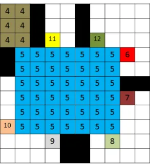
In this case, there is only 6 face centers (both side and shared center points are counted), and the sum of combined distances between these central points equals to 42 (there are

The performance of the ALE under different parameters such as the step size, filter ‎length, and SNR has been studied extensively by simulations and experiments when

architectural design (traditional media: paper-based drawings and physical scale models; and digital media) are analyzed in terms of their capacity to support dynamic

In order to use negative bag constraints of Multiple Instance Learn- ing, it must be made sure that the constructed negative bags do not con- tain any positive instances. For