Fast Computation of the Ambiguity Function and the
Wigner Distribution on Arbitrary Line Segments
Ahmet Kemal Özdemir, Student Member, IEEE, and Orhan Arıkan, Member, IEEE
Abstract—By using the fractional Fourier transformation of the
time-domain signals, closed-form expressions for the projections of their auto or cross ambiguity functions are derived. Based on a sim-ilar formulation for the projections of the auto and cross Wigner distributions and the well known two-dimensional (2-D) Fourier transformation relationship between the ambiguity and Wigner domains, closed-form expressions are obtained for the slices of both the Wigner distribution and the ambiguity function. By using dis-cretization of the obtained analytical expressions, efficient algo-rithms are proposed to compute uniformly spaced samples of the Wigner distribution and the ambiguity function located on arbi-trary line segments. With repeated use of the proposed algorithms, samples in the Wigner or ambiguity domains can be computed on non-Cartesian sampling grids, such as polar grids.
Index Terms—Ambiguity function, fast computation, fractional
Fourier transformation, Wigner distribution.
I. INTRODUCTION
T
IME-FREQUENCY signal processing is one of the fun-damental research areas in signal processing. The Wigner distribution (WD) plays a central role in the theory and prac-tice of time-frequency signal processing [1]–[10]. Likewise, the ambiguity function (AF), which is the two-dimensional (2-D) Fourier transform of the Wigner distribution, plays a central role in time-frequency signal analysis [11]–[13] and radar and sonar signal processing [14]–[17].Because of the availability of efficient computational algo-rithms, both the WD and AF are usually computed on Cartesian grids [1], [18], [19]. In this paper, by using the fractional Fourier transformation of the time-domain signals, closed-form expressions for the projections of their auto or cross ambiguity functions are derived. Based on a similar formulation for the projections of the auto and cross Wigner distributions [20] and the well-known 2-D Fourier transformation relationship between the ambiguity and Wigner domains, novel closed-form expressions are obtained for the slices of both the WD and the AF. By using discretization of the obtained analytical expres-sions, efficient algorithms are proposed to compute uniformly spaced samples of the WD and the AF located on arbitrary line segments. With repeated use of these algorithms, it is possible to obtain samples of the WD and AF on non-Cartesian grids, such as polar grids that are the natural sampling grids
Manuscript received March 29, 1999; revised October 3, 2000. The associate editor coordinating the review of this paper and approving it for publication was Prof. Gregori Vazquez.
The authors are with the Department of Electrical and Electronics Engineering, Bilkent University, Ankara, Turkey (e-mail: [email protected] .edu.tr;[email protected]).
Publisher Item Identifier S 1053-587X(01)00620-1.
of chirp-like signals. The ability of obtaining WD and AF samples over polar grids is potentially very useful in various important application areas including time-frequency domain kernel design, multicomponent signal analysis, time-frequency domain signal detection, and particle location analysis in Fresnel holograms [21]–[28].
The organization of the paper is in accordance with the dual nature of the ambiguity function and Wigner distribution. We first provide some preliminaries on these important concepts. In Section III, by using the Radon-Wigner transformation, an-alytical expressions are derived for the slices of the auto am-biguity functions. Then, by discretizing the obtained analytical expressions, efficient algorithms are presented for the computa-tion of slices of the ambiguity funccomputa-tion. In Seccomputa-tion IV, we follow a similar development, leading to novel closed-form expressions for the Radon-ambiguity function, and present efficient algo-rithms for the computation of slices of the Wigner distribution. In Section V, both the analytical and computational results are extended to the cross AF and WD. In Section VI, we provide results of simulated applications of the proposed algorithms. Fi-nally, the paper is concluded in Section VII.
II. PRELIMINARIES ON THEWIGNERDISTRIBUTION AND THE AMBIGUITYFUNCTION
Discrete time-frequency analysis is the primary investiga-tion tool in the synthesis, characterizainvestiga-tion, and filtering of time-varying signals. Among the alternative time-frequency analysis algorithms, those belonging to the Cohen’s class are the most commonly utilized ones. In this class, the time-fre-quency distributions of a signal are given by1
TF
(1) where the function is called the kernel [4], [29]. Recent research on the time–frequency signal analysis has revealed that signal dependent choice of the kernel helps in localization of the time-frequency components of the signals [11], [21]–[24]. By choosing , the most commonly used member of the Cohen’s class (the Wigner distribution) is obtained
(2) Because of its nice energy localization properties, the WD has found important application areas. Definition (2) has been
gen-1All integrals are from01 to +1 unless otherwise stated.
eralized to define the cross-Wigner distribution of two signals
and as
(3) The properties of the cross-Wigner distribution have been inves-tigated in detail [1], [2]. Note that holds. The 2-D inverse Fourier transform (FT) of the WD is called the (symmetric) ambiguity function, and it has found important application areas including time-frequency signal analysis and radar signal processing
(4a) (4b) Similar to the cross-Wigner distribution, the cross-ambiguity function of two signals is defined as
(5) As in (4a), the ambiguity function is related to the cross-Wigner distribution through the 2-D inverse Fourier transforma-tion
(6)
III. FASTCOMPUTATION OF THEAMBIGUITYFUNCTION ON ARBITRARYLINESEGMENTS
In this section, an efficient algorithm to compute the ambi-guity function on uniformly spaced samples along an arbitrary line segment is provided. For the sake of simplicity, a gradual method of presentation is used where we first consider obtaining uniformly spaced samples of the AF on a line segment centered at the origin. Then, we extend this approach to obtain samples on a line segment positioned radially. Finally, we consider the case of an arbitrary line segment. The presentation of the posed approach will be as follows: First, the well-known pro-jection-slice relationship between the WD and the AF domains will be given. Then, the projections in the WD domain will be related to the fractional Fourier transformation of the signals in-volved. Finally, the obtained continuous-time relationship will be discretized to allow the use of a fast fractional Fourier trans-formation algorithm.
A. Radon–Wigner Transform
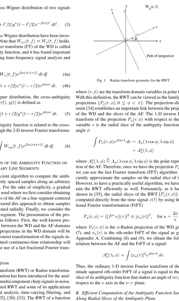
The Radon–Wigner transform (RWT) or Radon transforma-tion of the Wigner distributransforma-tion has been introduced for the anal-ysis and classification of multicomponent chirp signals in noise. Several authors investigated RWT and some of its applications in multicomponent signal analysis, time-varying filtering, and adaptive kernel design [25], [30]–[33]. The RWT of a function is defined as the Radon transform of its WD. Using the ge-ometry in Fig. 1, RWT can be written as
(7)
Fig. 1. Radon transform geometry for the RWT.
where are the transform domain variables in polar format. With this definition, the RWT can be viewed as the family of the
projections . The projection-slice
the-orem [34] establishes an important link between the projections of the WD and the slices of the AF. The 1-D inverse Fourier transform of the projection with respect to the radial variable is the radial slice of the ambiguity function at the angle
(8a) (8b)
where is the polar
representa-tion of the AF. Therefore, once we have the projecrepresenta-tion , we can use the fast Fourier transform (FFT) algorithm to effi-ciently approximate the samples on the radial slice of the AF. However, to have a practically useful algorithm, we have to ob-tain the RWT efficiently as well. Fortunately, as it has been shown in [35], the radial slices of the RWT [ ] can be computed directly from the time signal by using the frac-tional Fourier transformation (FrFT)
for (9)
where is the -Radon projection of the WD given by (7), and is the th-order FrFT of the signal as given in Appendix A. Combining (8) and (9), we obtain the following relation between the AF and the FrFT of a signal:
(10) Thus, the ordinary 1-D inverse Fourier transform of the mag-nitude squared th-order FrFT of a signal is equal to the radial slice of its ambiguity function that makes an angle of with respect to the axis in the – plane.
B. Efficient Computation of the Ambiguity Function Samples Along Radial Slices of the Ambiguity Plane
In this section, we provide the details of a fast algorithm for computing radial samples of the ambiguity function. As it will be shown in detail, for an input sequence of length , it is pos-sible to compute the samples of AF on an arbitrary line segment
centered at the origin in flops.2 We start with the
approximation of the integral in (10) with its uniform Riemann summation. For an equally valid approximation at all angles , in the rest of this paper, we assume that prior to obtaining its samples, is scaled so that its Wigner domain support is ap-proximately confined into a circle with radius centered at the origin. In other words, any th-order FrFT of , including the signal itself and its ordinary Fourier transform, has negli-gible energy outside the symmetric interval . For a signal with approximate time and frequency supports of and , respectively, the required scaling is , where
[36].
After the scaling, the double-sided bandwidth of is . Therefore, its inverse FT given in (10) can be expressed in terms of its uniformly obtained samples at a rate using the following discrete-time inverse Fourier transform relation:3
(11) where is an arbitrary integer that is greater than , which is the time-bandwidth product of , and is the th sample of the FrFT . To obtain equally spaced radial samples of , we substitute in the above equation:
(12)
After the discretization, the obtained form lends itself for an efficient digital computation since the required samples of the
FrFT [ ] can be computed
using the recently developed fast computation algorithm [36] in flops. The summation in (12) can be recast into a -point discrete Fourier transformation (DFT), which can be computed in flops using the fast Fourier transform algorithm. Therefore, the overall cost of computing the samples of the AF along any radial slice is flops.
Note that the relationship in (12) is discrete in the radial vari-able and continuous in the angular variable . By discretizing the angular variable, the samples of the AF along several radial lines can be computed. For instance, if this algorithm is used for a uniformly distributed set of angles
, covering the range , then the samples of the AF lo-cated on a polar grid can be computed in flops. In Fig. 3(a), we illustrate the shape of a polar grid on which the samples of the AF can be computed by using this al-gorithm.
2Complex multiplication and addition.
3From this observation, we deduce the following fact: If the WD ofx(t) is
confined into a circle with radius1 =2 in the Wigner plane, then its AF is confined into a circle with radius1 in the ambiguity plane.
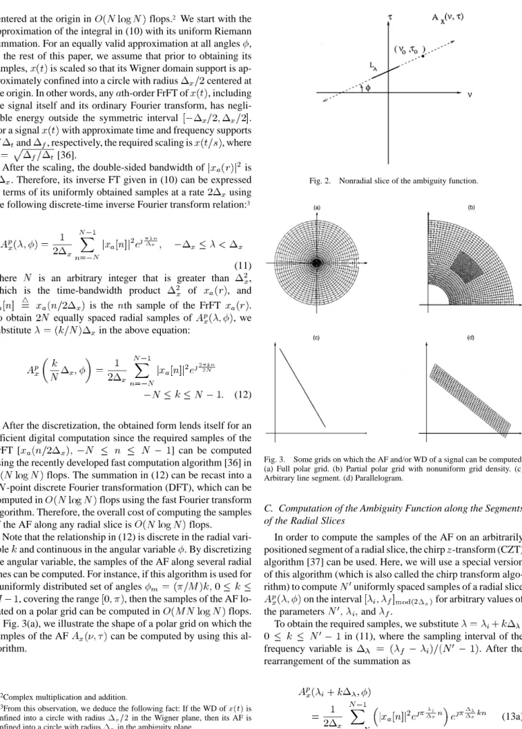
Fig. 2. Nonradial slice of the ambiguity function.
Fig. 3. Some grids on which the AF and/or WD of a signal can be computed. (a) Full polar grid. (b) Partial polar grid with nonuniform grid density. (c) Arbitrary line segment. (d) Parallelogram.
C. Computation of the Ambiguity Function along the Segments of the Radial Slices
In order to compute the samples of the AF on an arbitrarily positioned segment of a radial slice, the chirp -transform (CZT) algorithm [37] can be used. Here, we will use a special version of this algorithm (which is also called the chirp transform algo-rithm) to compute uniformly spaced samples of a radial slice on the interval for arbitrary values of
the parameters and .
To obtain the required samples, we substitute
in (11), where the sampling interval of the
frequency variable is . After the
rearrangement of the summation as
(13b)
where and are defined as
(14) (15)
we use the identity in (13b)
and obtain an alternative but equivalent expression for
(16) In this expression, can be interpreted as the convolution of the chirp-modulated signal and the chirp multiplied with another chirp . Since the convolution can be computed efficiently by using the FFT algorithm, for the usual case of , the uniformly spaced samples of the radial slice located in the segment
can be obtained in flops. In
Fig. 3(b), we illustrate the shape of a partial polar grid, on which the samples of the AF can be computed by using the algorithm of the previous section combined with the CZT algorithm. In this plot, the polar grid has denser samples in the middle region. The samples on the radial slices that pass through both the denser and nondenser parts of the grid can be obtained by using the CZT algorithm three times: once to compute the samples in the denser region and twice to compute the samples in the nondenser regions.
D. Computation of the Ambiguity Function Along Arbitrary Line Segments
In this section, we present a fast computational algorithm that computes the samples of AF on a nonradial slice. Let us consider the case of computing the samples of the AF along the line segment shown in Fig. 2. The following parameteriza-tion for the line segment will be used in the derivations:
(17) where is an arbitrary point that lies on , and is the angle between and the axis. Using this parameterization of and the definition of the AF, the nonradial slice of the AF that lies on the line segment can be written as
(18a) (18b)
where is the cross-ambiguity function of the fol-lowing time-domain signals and :
(19) (20) Thus, the nonradial slice of is equal to the radial slice of the , where both of the slices are in parallel. Hence, similar to (8), the projection-slice theorem can be used to ex-press the slice of the along the line segment as the 1-D inverse FT of the -Radon projection of the corresponding cross-Wigner distribution
(21) We note that analogous to (9), the -Radon projections of the cross WD can be obtained from the following FrFT relation [20]:
(22) where is the FrFT order. Then, following the discus-sions in Sections III–B and C, we obtain the following expres-sion for the uniformly spaced samples of the AF on the line segment
(23)
where . As in the last section,
these samples of the AF on the nonradial line segment can be computed using the chirp transform algorithm.
IV. FASTCOMPUTATION OF THEWIGNERDISTRIBUTION ON ARBITRARYLINESEGMENTS
In the rest of this paper, we will present the dual development for the Wigner distribution. In the next section, we introduce the dual of the Radon-Wigner transform: the Radon-ambiguity function transform (RAFT). Then, we derive the relationship be-tween the RAFT and FrFT. As in the computation of the AF samples, this relationship will naturally lead us to the fast com-putation algorithm for the required WD samples.
A. Radon-Ambiguity Transform
The Radon transformation has been found to be a useful tool in time–frequency signal processing with applications to detec-tion of chirp rates [26] and signal-dependent kernel design [24]. As we show in the following sections, the Radon transform of the ambiguity function itself is also an important tool in the ef-ficient computation of the WD slices.
Here, we introduce the Radon-ambiguity function transform of a signal as the Radon transform of its ambiguity function. The RAFT can be written as
where are the polar format variables. Using the projection-slice theorem, the radial projection-slice of the WD at an angle can be written as the FT of with respect to the radial variable
(25a) (25b)
where is the polar
represen-tation of the WD.
To obtain a fast computational algorithm similar to that in Section III-B, the samples of the projections have to be obtained efficiently. In the next section, we investigate the relationship between the RAFT and the FrFT.
B. Relation Between the Radon-Ambiguity Function Transformation and the Fractional Fourier Transformation
The relationship of the RWT to the FrFT is well known in the literature. In this section, we show that a similar relationship ex-ists between the RAFT and FrFT. We start with the substitution of (4b) into (24), resulting in the following expression for the radial slice of the RAFT:
(26a)
(26b) By making the following change in the integration variables:
(27) (28) the integral in (26b) can be written as in the following separable form:
(29) By using the definition of given in (56), it follows that . After substituting this identity into (29), the separated terms can be written in the form of FrFT
(30a)
(30b) (30c)
where is the FrFT order. Thus,
com-bining (25) with (30) and discretizing the obtained relationship, we obtain an algorithm that can be used to compute the samples of the WD on polar grids, such as the ones shown in Figs. 3(a) and (b). In the following section, based on the above relation-ship, we propose an efficient algorithm to compute samples of the WD on arbitrary line segments.
C. Computation of the Wigner Distribution along Arbitrary Line Segments
Suppose that we want to compute samples of the WD of a waveform along an arbitrary line segment in the Wigner plane. Since the line segment may not pass through the origin, we cannot immediately use the results of the pre-vious section. However, as in Section III-D, we will express the required nonradial slice as the radial slice of the WD of another function that allows us to use the results of the previous section. In the following derivation, we parameterize the line segment
as
(31) In this expression, is an arbitrary point that lies on , and is the angle of with the axis. Using this parameter-ization of , the nonradial slice of the WD can be expressed as
(32a) (32b) where is the radial slice of the WD of
(33) Hence, the nonradial slice of the WD of is the same as the radial slice of the WD of the time-shifted and frequency-modulated version of it, where both slices are in parallel. By using the projection-slice theorem given in (25), the nonradial slice of the WD of can be obtained as
(34) where is the -Radon projection of the ambiguity func-tion . Since the required -Radon projection satisfies the following FrFT relationship:
(35) where , it can be efficiently computed by using the fast FrFT algorithm proposed in [36] and given here as Algorithm 1. The steps of the proposed algorithm are given in Algorithm 3. Note that unlike , which is the -Radon
Algorithm 1. Fast fractional Fourier transform algorithm proposed in [36].
projection of the WD given by (7), the double-sided bandwidth
of is .
V. FASTCOMPUTATION OF THECROSSAMBIGUITYFUNCTION AND THECROSSWIGNERDISTRIBUTION ONARBITRARYLINE
SEGMENTS
Up to now, our main objective was developing algorithms for efficient computation of the samples of the AF and WD on arbi-trary line segments. However, in some applications [14], [38], it is required to compute the cross AF and the cross WD of a pair of given signals. As we show below, the same algorithms, with some slight modifications, can still be used to compute samples of the cross AF and the cross WD on arbitrary line segments ef-ficiently.
A. Fast Computation of the Cross Ambiguity Function on Arbitrary Line Segments
Suppose that we want to compute the samples of the cross AF of the two signals and on the line segment shown in Fig. 2. This nonradial slice of the cross AF function is given as
(36a) (36b)
Algorithm 2. Fast computation of the cross-ambiguity function on arbitrary line segments.
Algorithm 3. Fast computation of the cross-Wigner distribution on arbitrary line segments.
where is the radial slice of the cross AF of the signals and
(37) (38)
The radial slice of the is the 1-D inverse FT of the -Radon projection of the
where the -Radon projection satisfies the following relation with the FrFTs of and
(40) Then, the required nonradial slice of the can be ob-tained as
(41) Discretization of this expression yields the fast computational algorithm.
B. Fast Computation of the Cross Wigner Distribution on Arbitrary Line Segments
In this section, we derive the algorithm for fast computation of the samples of the on an arbitrary line segment as parameterized in (31). This nonradial slice of the cross WD can be expressed as the radial slice of
(42a) (42b) where the signals and are defined as
(43) (44) Using the projection-slice theorem, this radial slice of the can be expressed as the 1-D FT of the -Radon
projection of the
(45) where the -Radon projection is given in terms of the
th-order FrFTs of the signals and
(46) Finally, substituting (45) and (46) into (42) gives
(47) Discretization of this expression as in (23) yields the fast com-putational algorithm.
VI. SIMULATIONS
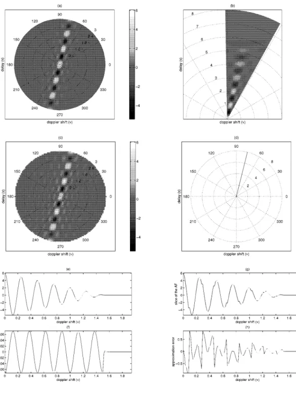
In this section, by using simulations, we will investigate the performance of the proposed algorithms. For this purpose, we consider the signals with analytically known ambiguity functions and Wigner distributions. This way, we will be able to investigate the error due to discretization of the fractional Fourier transformation on the obtained samples. First, we will investigate the performance of Algorithm 2, which computes the samples of the ambiguity function on arbitrary line segments. In this simulation, we use a linear-fre-quency modulated chirp signal with a rectangular envelope rect , where the rect function takes
the value 1 if its argument falls into the range is the rate of the chirp, and is its initial phase. The corresponding ambiguity function has the following closed-form expression:
sinc
rect (48)
In the simulation performed here, the values of the
parame-ters are chosen as and . Then, by
sampling at a rate , we obtained
uni-formly spaced samples in the interval . Since the significant energy of the th-order FrFTs of are con-fined into this interval, no scaling is applied to the continuous time signal . In other words, the value of the scaling param-eter is given as , which is also true for the other simulations in this section. In Fig. 4(a), Algorithm 2 is used to compute the AF samples on the full polar grid with the angular spacing of rad and radial spacing of normalized units. As shown in Fig. 4(b), by using the same algorithm, samples of the AF can also be obtained over a partial polar grid with the same angular and radial sampling intervals. For the display pur-pose, the AF of the same signal could also be computed on a Cartesian grid. In this simulation, the AF is first computed by using the algorithm in [18] on the whole Cartesian grid with Doppler and delay spacings of units. Then, in Fig. 4(c), real parts of the computed AF samples that reside on a circular disk with radius 3 are plotted. To investigate the accuracy of the proposed algorithm, we computed in flops the samples of the ambiguity function of the same chirp pulse over the radial line segment shown in Fig. 4(d). The real parts of the computed samples and their deviation from the samples com-puted by using (48) are shown in Fig. 4(e) and (f), respectively. As it can be seen from this example, the computed samples are highly accurate. Alternatively, the samples on the line segment shown in Fig. 4(d) could be approximated from the computed AF samples on the Cartesian grid by using a crude interpolator such as the nearest neighbor interpolator. The result of this al-ternative approach is shown in Fig. 4(g), where the real parts of the computed samples are plotted. With the comparison of the approximation errors in Fig. 4(f) and (h), it becomes apparent that the new algorithm produces a ten-times more accurate re-sult for this simulation. Furthermore, when the line segment has arbitrary orientation with samples on it, the alternative computation based on the Cartesian grid requires
flops. On the other hand, by using Algorithm 2, the same AF samples can be computed with ten times more accuracy in only
flops.
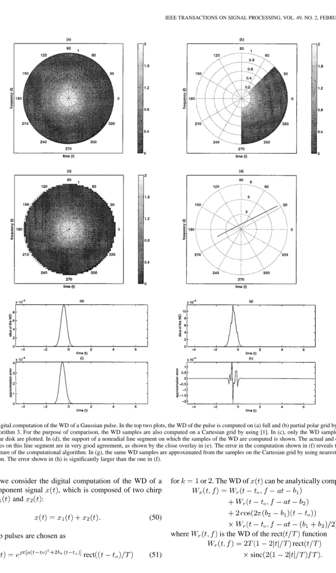
Next, we investigate the accuracy of the algorithms in com-puting the WD of the Gaussian pulse , which has the Wigner distribution
(49)
By sampling at a rate , we obtained
uniformly spaced samples in the interval . Fig. 5(a) and (b) are obtained by repeated application of the Algorithm 3. In (a), the WD is computed over a full, and in (b), it is computed over a partial polar grid. For the purpose of comparison, the WD samples are also computed on a Cartesian grid by using the algorithm in [1] with a sampling interval of
Fig. 4. Digital computation of the AF of a chirp signal with a rectangular envelope: In the top two plots, the real part of the AF of the pulse is computed on (a) full and (b) partial polar grid by repeated use of the Algorithm 2. For the purpose of comparison, the AF samples are also computed on a Cartesian grid by using [18]. In (c), the real parts of these AF samples that lie on a circular disk are plotted. In (d), the support of a radial line segment on which the samples of the AF are computed is shown. The real parts of the actual and computed AF samples on this line segment by using Algorithm 2 are in very good agreement, as shown by the close overlay in (e). The error in the computation shown in (f) reveals the highly accurate nature of the computational algorithm. In (g), the same AF samples are approximated from the samples on the Cartesian grid by using nearest neighbor interpolation. The peak approximation error in (h) is approximately ten times larger than the one in (f).
units both in time and frequency. Then, in Fig. 5(c), only the WD samples that lie on a circular disk with radius 1 are plotted.
To show the accuracy of the proposed algorithm, we com-puted, in flops, samples of the Wigner distribu-tion of the same Gaussian pulse over the nonradial line segment shown in Fig. 5(d). The obtained samples and the approximation error are plotted in Fig. 5(e) and (f), respectively. For the purpose
of comparison, the same AF samples are approximated from the Cartesian grid samples by using nearest neighbor interpolation. In Fig. 5(g), the approximated and actual AF samples are shown, and in Fig. 5(h), the computation error is shown. As in the AF case presented above, not only the accuracy of the computed samples shown in Fig. 5(h) is significantly less than the accu-racy obtained by using Algorithm 3, but also the computation of the Cartesian grid based algorithm requires flops.
Fig. 5. Digital computation of the WD of a Gaussian pulse. In the top two plots, the WD of the pulse is computed on (a) full and (b) partial polar grid by repeated use of Algorithm 3. For the purpose of comparison, the WD samples are also computed on a Cartesian grid by using [1]. In (c), only the WD samples that lie on a circular disk are plotted. In (d), the support of a nonradial line segment on which the samples of the WD are computed is shown. The actual and computed WD samples on this line segment are in very good agreement, as shown by the close overlay in (e). The error in the computation shown in (f) reveals the highly accurate nature of the computational algorithm. In (g), the same WD samples are approximated from the samples on the Cartesian grid by using nearest neighbor interpolation. The error shown in (h) is significantly larger than the one in (f).
Next, we consider the digital computation of the WD of a multicomponent signal , which is composed of two chirp
pulses and
(50) The chirp pulses are chosen as
rect (51)
for or . The WD of can be analytically computed as
(52) where is the WD of the rect function
rect
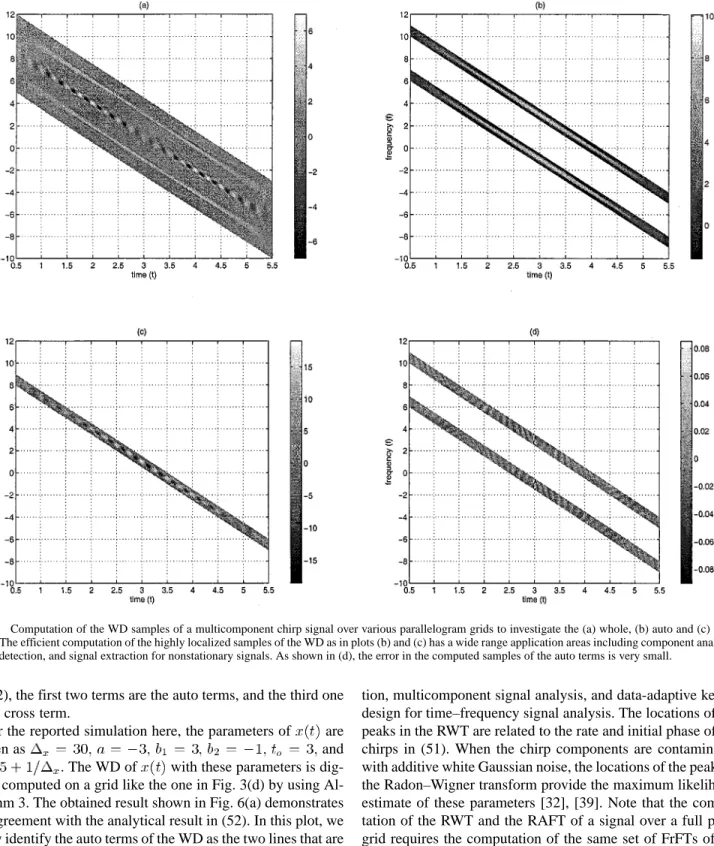
Fig. 6. Computation of the WD samples of a multicomponent chirp signal over various parallelogram grids to investigate the (a) whole, (b) auto and (c) cross terms. The efficient computation of the highly localized samples of the WD as in plots (b) and (c) has a wide range application areas including component analysis, signal detection, and signal extraction for nonstationary signals. As shown in (d), the error in the computed samples of the auto terms is very small.
In (52), the first two terms are the auto terms, and the third one is the cross term.
For the reported simulation here, the parameters of are
chosen as and
. The WD of with these parameters is dig-itally computed on a grid like the one in Fig. 3(d) by using Al-gorithm 3. The obtained result shown in Fig. 6(a) demonstrates the agreement with the analytical result in (52). In this plot, we easily identify the auto terms of the WD as the two lines that are closer to the edges, and we identify the cross term as the line that is at the middle part of the plot. The cross term is highly oscilla-tory because of the cosine modulation in (52). In Fig. 6(b) and (c), computed samples of the auto and cross terms are shown over highly localized grids of the type given in Fig. 3(d). Fi-nally, in Fig. 6(d), we provide the approximation error for the auto terms only.
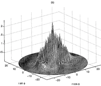
In Fig. 7, the Radon-Wigner transform and Radon-ambiguity function transform of the same multicomponent signal are com-puted on polar grids by using the FrFT relations (9) and (30). These transforms have important applications in signal
detec-tion, multicomponent signal analysis, and data-adaptive kernel design for time–frequency signal analysis. The locations of the peaks in the RWT are related to the rate and initial phase of the chirps in (51). When the chirp components are contaminated with additive white Gaussian noise, the locations of the peaks in the Radon–Wigner transform provide the maximum likelihood estimate of these parameters [32], [39]. Note that the compu-tation of the RWT and the RAFT of a signal over a full polar grid requires the computation of the same set of FrFTs of the signal. Hence, when these transforms are to be calculated simul-taneously, significant computational savings can be achieved by avoiding any extra computation of the FrFT samples.
VII. CONCLUSION
By using the FrFT of the time-domain signals, closed-form expressions for the projections of their auto or cross ambiguity functions are derived. Based on a similar formulation for the projections of the auto and cross Wigner distributions and the well-known 2-D Fourier transformation relationship between
Fig. 7. Digital computation of the (a) Radon–Wigner transform and (b) magnitude of the Radon-ambiguity function transform. In this paper, the computation of these transforms constitute the intermediate steps in computation of the ambiguity function and the Wigner distribution on polar grids.
the ambiguity and Wigner domains, closed-form expressions are obtained for the slices of both the Wigner distribution and the ambiguity function. Based on the obtained analytical results, ef-ficient algorithms are proposed for the computation of the auto or cross Wigner distribution and ambiguity function samples on arbitrary line segments. The proposed algorithms make use of a digital computation algorithm of the FrFT to compute uni-formly spaced samples in flops. The ability of ob-taining samples on arbitrary line segments provides significant flexibility in the computational applications involved with the Wigner distribution and the ambiguity function.
APPENDIX A
FRACTIONALFOURIERTRANSFORMATION
The th-order, , FrFT of a function
is defined as [40]
(54) where the kernel of the transformation is
(55) (56) (57) The transformation kernel is the complex exponential
for , and it approaches for and to
for . Thus, it follows that the first-order FrFT is the ordinary Fourier transform, and the zeroth-order FrFT is the function itself. The definition of the FrFT is easily extended to outside the interval by noting that is the identity operator for any integer and the FrFT is additive in the index,
i.e., .
REFERENCES
[1] T. A. C. M. Claasen and W. F. G. Mecklenbrauker, “The Wigner dis-tribution—A tool for time-time frequency signal analysis, part II: Dis-crete-time signals,” Philips J. Res., vol. 35, no. 4/5, pp. 276–350, 1980. [2] T. A. C. Claasen and W. F. G. Mecklenbrauker, “The aliasing problem in discrete-time Wigner distributions,” IEEE Trans. Acoust., Speech,
Signal Processing, vol. ASSP-31, pp. 1067–1072, Oct. 1983.
[3] G. F. Boudreaux-Bartels and T. W. Parks, “Time-varying filtering and signal estimation using Wigner distribution synthesis techniques,” IEEE
Trans. Acoust., Speech, Signal Processing, vol. ASSP-34, pp. 442–451,
June 1986.
[4] L. Cohen, “Time-frequency distributions—A review,” Proc. IEEE, vol. 77, pp. 941–981, July 1989.
[5] F. Hlawatsch and G. F. Boudreaux-Bartels, “Linear and quadratic time-frequency signal representations,” IEEE Signal Processing Mag., vol. 9, pp. 21–67, Apr. 1992.
[6] W. F. G. Mecklenbrauker, Ed., The Wigner Distribution-Theory and
Ap-plications in Signal Processing. New York: Elsevier, 1992. [7] L. R. Dragonette, D. M. Drumheller, C. F. Gaumond, D. H. Hughes, B.
T. O’connor, N. Yen, and T. J. Yoder, “The application of two-dimen-sional signal transformations to the analysis and synthesis of structural excitations observed in acoustical scattering,” Proc. IEEE, vol. 84, pp. 1249–1263, Sept. 1996.
[8] P. K. Kumar and K. M. M. Prabhu, “Simulation studies of moving-target detection: A new approach with Wigner-Ville distribution,” Proc. Inst.
Elect. Eng., Radar. Sonar Navig., vol. 144, no. 5, pp. 259–265, Oct.
1997.
[9] S. Haykin and D. J. Thomson, “Signal detection in nonstationary en-vironment reformulated as an adaptive pattern classification problem,”
Proc. IEEE, vol. 86, pp. 2325–2344, Nov. 1998.
[10] V. Katkovnik and L. Stankovic, “Instantaneous frequency estimation using the Wigner distribution with varying data-driven window length,”
IEEE Trans. Signal Processing, vol. 46, pp. 3215–2325, Sept. 1998.
[11] P. Flandrin, “Some features of time-frequency representations of mul-ticomponent signals,” in Proc. IEEE Int. Conf. Acoust., Speech, Signal
Process., vol. 3, 1984, pp. 41B.4.1–41B.4.4.
[12] P. Bonato, A. Destefano, and R. Ceravolo, “Time-frequency and am-biguity function approaches in structural identification,” ASCE J. Eng.
Mech., vol. 123, no. 12, pp. 1260–1267, 1997.
[13] S. Parsons, C. W. Thorpe, and S. M. Dawson, “Echolocation calls of the long-tailed bat—A quantitative analysis of types of calls,” J. Mammol., vol. 78, no. 3, pp. 946–976, 1997.
[14] P. M. Woodward, Probability and Information Theory, with Applications
to Radar. New York: Pergamon, 1953.
[15] C. H. Wilcox, “The synthesis problem for radar ambiguity functions,”, MRC Tech. Summary Rep. 157, Apr. 1960.
[16] R. E. Blahut, W. Miller, and C. H. Wilcox Jr., Radar and Sonar. New York: Springer-Verlag, 1991, vol. 32.
[17] G. C. Gaunaurd and H. C. Strifors, “Signal analysis by means of time-frequency (Wigner-type) distributions—Applications to sonar and radar echos,” Proc. IEEE, vol. 84, pp. 1231–1248, Sept. 1996.
[18] S. M. Sussman, “Least-squares synthesis of radar ambiguity functions,”
IRE Trans. Inform. Theory, vol. IT-8, pp. 246–254, Apr. 1962.
[19] G. S. Cunningham and W. J. Williams, “Fast implementations of gener-alized discrete time-frequency distributions,” IEEE Trans. Signal
Pro-cessing, vol. 42, pp. 1496–1508, June 1994.
[20] I. Raveh and D. Mendlovic, “New properties of the Radon transform of the cross Wigner/ambiguity distribution function,” IEEE Trans. Signal
Processing, vol. 47, pp. 2077–2080, July 1999.
[21] R. G. Baraniuk and D. L. Jones, “A signal-dependent time-frequency representation: Optimal kernel design,” IEEE Trans. Signal Process., vol. 41, pp. 1589–1601, Apr. 1993.
[22] , “A signal-dependent time-frequency representation: Fast algo-rithm for optimal kernel design,” IEEE Trans. Signal Processing, vol. 42, pp. 134–146, Jan. 1994.
[23] , “An adaptive optimal-kernel time-frequency representation,”
IEEE Trans. Signal Process., vol. 43, pp. 2361–2371, Oct. 1995.
[24] B. Ristic and B. Boashash, “Kernel design for time-frequency signal analysis using the Radon transform,” IEEE Trans. Signal Processing, vol. 41, pp. 1996–2008, May 1993.
[25] S. Barbarossa, “Analysis of multicomponent LFM signals by a com-bined Wigner-Hough transform,” IEEE Trans. Signal Processing, vol. 43, pp. 1511–1515, June 1995.
[26] M. Wang, A. K. Chan, and C. K. Chui, “Linear frequency-modulated signal detection using Radon-ambiguity transform,” IEEE Trans. Signal
Processing, vol. 46, pp. 571–586, Mar. 1998.
[27] M. T. Ozgen and K. Demirbas, “Cohen’s bilinear class of shift-invariant space/spatial-frequency signal representations for particle-location anal-ysis of in-line Fresnel holograms,” J. Opt. Soc. Amer. A, vol. 15, no. 8, pp. 2117–2137, Aug. 1998.
[28] M. T. Ozgen, “An automatic kernel design procedure for the Cohen’s bilinear class of representations as applied to in-line Fresnel holograms”, submitted for publication.
[29] L. Cohen, Time-Frequency Analysis. Englewood Cliffs, N.J.: Prentice-Hall, 1995.
[30] J. C. Wood and D. T. Barry, “Tomographic time-frequency analysis and its application toward time-varying filtering and adaptive kernel desing for multicomponent linear-FM signals,” IEEE Trans. Signal Processing, vol. 42, pp. 2094–2104, Aug. 1994.
[31] , “Linear sinal synthesis using the Radon-Wigner transform,” IEEE
Trans. Signal Processing, vol. 42, pp. 2105–2111, Aug. 1994.
[32] , “Radon transformation of time-frequency distributions for anal-ysis of multicomponent signals,” IEEE Trans. Signal Processing, vol. 42, pp. 3166–3177, Nov. 1994.
[33] Z. Bao, G. Wang, and L. Luo, “Inverse synthetic aperture radar imaging of maneuvering targets,” Opt. Eng., vol. 37, no. 5, pp. 1582–1588, May 1998.
[34] R. N. Bracewell, Two-Dimensional Imaging. Englewood Cliffs, NJ: Prentice-Hall, 1995.
[35] A. W. Lohmann and B. H. Soffer, “Relationships between the Radon-Wigner and fractional Fourier transforms,” J. Opt. Soc. Amer. A, vol. 11, pp. 1798–1801, 1994.
[36] H. M. Ozaktas, O. Arıkan, M. A. Kutay, and G. Bozdagi, “Digital com-putation of the fractional Fourier transform,” IEEE Trans. Signal
Pro-cessing, vol. 44, pp. 2141–2150, Sept. 1996.
[37] L. R. Rabiner, R. W. Schafer, and C. M. Rader, “The chirp z-trans-form algorithm and its applications,” Bell Syst. Tech. J., vol. 48, pp. 1249–1292, May 1969.
[38] T. J. McHale and G. F. Boudreaux-Bartels, “An algorithm for syn-thesizing signals from partial time-frequency models using the cross Wigner distribution,” IEEE Trans. Signal Processing, vol. 41, pp. 1986–1990, May 1993.
[39] S. Kay and G. F. Boudreaux-Bartels, “On the optimality of the Wigner distribution for detection,” in Proc. IEEE Int. Conf. Acoust. Speech,
Signal Process., vol. 3, Mar. 1985, pp. 1017–1020.
[40] V. Namias, “The fractional order Fourier transform and its application to quantum mechanics,” J. Inst. Math. Appl., vol. 25, pp. 241–265, 1980.
Ahmet Kemal Özdemir (S’97) was born in 1974
in Ankara, Turkey. He received the B.Sc. and M.S. degrees in electrical and electronics engineering from Bilkent University, Ankara, in 1996 and 1998, respectively. During his M.S. study, he was a Teaching and Research Assistant. He is currently pursuing the Ph.D. degree under the supervision of O. Arıkan with the Department of Electrical and Electronics Engineering, Bilkent University.
His research interests are in digital signal processing and its applications to time-frequency analysis, radar signal processing, and communications.
Orhan Arıkan (M’91) was born in 1964 in Manisa,
Turkey. He received the B.Sc. degree in electrical and electronics engineering from the Middle East Tech-nical University, Ankara, Turkey, in 1986 and both the M.S. and Ph.D. degrees in electrical and com-puter engineering from the University of Illinois, Ur-bana-Champaign, in 1988 and 1990, respectively.
Following his graduate studies, he worked for three years as a Research Scientist at Schlum-berger-Doll Research, Ridgefield, CT. During this time, he was involved in the inverse problems and fusion of measurements with multiple modality. He joined Bilkent University, Ankara, in 1993, where he is presently Associate Professor of electrical engineering. His current research interests are in adaptive signal processing, time–frequency analysis, inverse problems, and array signal processing.