Rescheduling frequency in an FMS with uncertain processing times and unreliable machines

(1)

Rescheduling Frequency in an FMS with

Uncertain Processing Times

and Unreliable Machines

Ihsan Sabuncuoglu, Dept. of Industrial Engineering, Bilkent University, Ankara, Turkey

Suleyman Karabuk, Dept. of Industrial Engineering, Lehigh University, Bethlehem, Pennsylvania

Abstract

This paper studies the scheduling/rescheduling problem in a multi-resource FMS environment. Several reactive scheduling policies are proposed to address the effects of machine breakdowns and processing time variations. Both off-line and on-line scheduling methods are tested under a variety of experimental conditions. The performance of the system is measured for mean tardiness and makespan criteria. The relationships between scheduling frequency and other scheduling factors are investigated. The results indi- cated that a periodic response with an appropriate period length would be sufficient to cope with interruptions. It was also observed that machine breakdowns have more significant impact on the system performance than processing time variations. In addition, dispatching rules were found to be more robust to interruptions than the optimum-seeking off-line scheduling algorithm. A comprehensive bibliography is also included in the paper.

Keywords: Scheduling/Rescheduling, Reactive Control

Introduction

Most manufacturing systems operate in dynamic environments subject to various stochastic disturbances (such as machine breakdowns, arrival of hot jobs). These disturbances not only interrupt system operation but also upset the schedule that was previ- ously established. In response to these unexpected changes, various alternative courses of action are available to a scheduler, such as rescheduling, local modifications (or partial rescheduling), and so on. The choice of a particular response depends on a number of factors, ranging from the type and duration of disturbances to current workload and slack in the system. It also depends on how schedules are initially generated.

There are mainly two types o f scheduling schemes: off-line and on-line. Off-line scheduling refers to the scheduling of all operations of available jobs for the entire planning horizon, whereas on-line scheduling attempts to schedule operations one at a

time, as they are needed. Priority dispatching is a good example of on-line scheduling because decisions are made one at a time as the system state changes (such as by new arrivals, job completions, and so forth). These local decisions--selecting a job from the queue of a particular machine--are usually made very quickly, so scheduling decisions are delayed until the last moment in the on-line case. Hence, the term "real-time scheduling" is also used interchangeably with on-line scheduling, t However, real-time scheduling can also be accomplished by an off-line method. In this case, scheduling can be viewed as a scheduling/rescheduling process in which schedules are revised in response to unexpected events. In some cases, there may be sufficient slack in the system to absorb the negative impact of interruptions without needing any revision; however, in most cases these events affect the performance o f the system so that corrective actions need to be taken.

The main feature of the scheduling/rescheduling approach is to establish a schedule for all operations of all jobs in the system for a fixed time period in advance. 2 However, determining appropriate scheduling points (that is, points in time at which scheduling decisions are made) needs further investigation. In practice, too-frequent schedule revisions (such as changes in plans, requirements for new material, machine setup and manpower, reevaluation of due dates, and order expediting activities) can increase system nervousness. Rescheduling, too, seldom results in poor system performance as events that significantly alter system state are ignored by the scheduling procedure.

The purpose of this paper is to study the frequency of rescheduling in the multi-resource environment of a flexible manufacturing system (FMS) with random machine breakdowns and processing times.

(2)

Journal of MunufiTcturing 5~stems Vol. 18/No. 4 1999

Because the FMS scheduling problem requires global coordination of various resources in the system, the problem is studied under various experimental conditions: varying machine and AGV load levels, machine breakdown rates, buffer capacity, routing flexibility, and sequence flexibility. Hence, the relationships between scheduling frequency and other

scheduling factors are investigated.

Literature Review

The majority of the scheduling literature deals with the task of schedule generation. Most of these studies either propose a scheduling algorithm or test priority dispatch rules. However, in practice, schedule genera-

tion is only one aspect of the scheduling process. Reactive control is equally important for the success- ful implementation of scheduling systems. Especially in today's highly dynamic and competitive manufacturing environments, scheduling systems should not only be able to generate high-quality schedules but also to react quickly to unexpected changes and to revise schedules in a cost-effective manner.

A number of studies analyze scheduling problems in a dynamic and stochastic environment and propose reactive policies for shop floor control. This research can be classified under three categories: (1) scheduling/rescheduling (rolling horizon) approaches, (2) artificial intelligence and knowledge-based systems, and (3) simulation-based experimental studies and iterative simulation approaches.

Early work on reactive scheduling used the rolling horizon approach to address the dynamic nature of scheduling problems. In this approach, a series of

static and deterministic problems are solved and their solutions are implemented on a rolling horizon basis. This is also called the scheduling/rescheduling approach. The first study in this area is probably that of Nelson, Holloway, and Wong, 3 who develop a scheduling system for a job shop with intermittent job arrivals. Later, Muhlemann, Lockett, and Farn 4 investigate the scheduling frequency in a dynamic job shop environment with processing time variations and machine breakdowns. Yamamoto and Nof 2 study a rescheduling policy in a static scheduling environment with random machine breakdowns. Their policy consists of generating a complete schedule whenever a machine breakdown occurs. All these studies agree that a rescheduling approach constitutes a better reactive policy than the applica-

tion of dispatching rules and predetermined schedules without any sequence modification.

Bean et al. s propose another approach to cope with randomness. They argue that schedule revisions after the system has started can at best achieve the performance of the initially generated schedule (that is, the preschedule). They develop an algorithm with the objective of generating a schedule that will match up with the preschedule at some later point. Wu, Storer, and Chang 6 adopt a similar approach in a single-machine environment with random machine failures. Their algorithm optimizes the performance of the remaining schedule and minimizes the deviation from the previous schedule when applied at a rescheduling point.

Church and Uzsoy 7 study the problem ofreschedul- ing in a single-machine environment with dynamic job arrivals. According to their proposed policy, rescheduling takes place at fixed time intervals unless an urgent job triggers an early rescheduling. Once an urgent job arrives, an exceptional scheduling takes place. Later, Ovacik and Uzsoy 8 propose several rolling horizon procedures in a single-machine environment with sequence-dependent setups.

Leon, Wu, and Storer 9 define the problem as that of finding a good initial schedule that will also maintain its planned performance under stochastic disturbances. In a similar study, Daniels and Kouvelis 1° describe the stochasticity in terms of scenarios and redefine the scheduling problem as finding a sequence that minimizes the maximum deviation between the performance of that sequence and the associated optimum sequences over all scenarios. In a more recent study, Mehta and Uzsoy" develop an algorithm that minimizes maximum lateness and the difference between job completion times in the preschedule and the realized one. These studies indicate that schedules that are robust to stochastic disturbances can be generated without too much sacrifice from the performance of the schedule.

Automated systems (such as FMS and CIM) have accelerated research on reactive scheduling. In two similar studies, Chang, Matsuo, and Sullivan ~2 and Raman, Talbot, and Rachamadugu ~3 apply their proposed off-line scheduling algorithms to generate complete schedules at each job arrival in a FMS environment. In their approach, a static, deterministic scheduling problem is solved at each job arrival. These approaches are shown to be superior to dispatching rules.

(3)

A second area in which numerous publications have emerged in recent years is the application of artificial intelligence (AI) and knowledge-based systems (KBS). The basic motivation of these applications is that each scheduling system is unique, and therefore, a wide variety of technical expertise, system-specific knowledge, and human judgment must be incorporat- ed in their implementation. Knowledge-based systems focus on capturing the expertise of the human scheduler and using it as an input to the scheduling process (see, for example, Shaw, Park, and Raman, 14 McKay, Buzacott, and Safayeni, is and Dutta16).

There are several other AI-based systems in the literature. Among them, ISIS developed by Fox and Smith 17 and OPIS (see Ow, Potvin, and Muscettola TM and Smith ~9) can be considered as the most success- ful AI implementations in scheduling. Other related work and a discussion on knowledge-based tech- nologies can be found in Szelke and Kerr. 2°

Since a typical scheduling environment in practice is dynamic and requires continuous updates, discrete-event simulation models are also used for the reactive scheduling problems. For example, Kim and Kim zl propose a simulation-based scheduling system with two major components: simulation mechanism and reactive control. The simulation mechanism evaluates various rules and selects the best one for a given job population and performance criterion. The reactive control mechanism monitors the system operation periodically and determines the timing of new simulation runs. In another study, Kutanoglu and Sabuncuoglu z, develop a simulation- based scheduling system to investigate the performance of several queue routing strategies that are designed to cope with machine breakdowns.

Other studies analyze scheduling methods under certain stochastic events and variations, rather than developing reactive policies. He, Smith, and Dudek z3 examine the effects of processing time variations (PVs) on the performance of dispatch rules in a dynamic job shop. Their main result is that a moderate level of PV does not affect the relative performances of the rules. Lawrence and Sewell z4 investigate the effects of stochastic processing times on scheduling methods and find that as the variability increases, the fixed optimum sequence is outperformed by the heuristic algorithm and dispatch rules.

In most studies that investigate reactive scheduling problems, a static production environment (that

is, no new job arrivals) is assumed. Some of the studies focus on single-machine systems, whereas others model multi-machine production environments (such as job shop or FMS). It seems that off- line scheduling algorithms perform better than on- line dispatching rules in static and deterministic environments; however, their relative performance is not generally known in stochastic and dynamic environments. The results also indicate that scheduling/rescheduling is a viable reactive policy. However, the marginal improvement in system performance due to rescheduling decreases as the scheduling frequency increases (see Church and Uzsoy7). Previous studies also indicate that some heuristics (particularly dispatching rules) are more sensitive to the changes in the scheduling period. Moreover, as some researchers noted, under a particular scheduling period and level of uncertainty, the performance of the rules improves as the level of congestion decreases. The purpose of this study is to reinvestigate this problem in a more general environment (such as an FMS) so that some earlier results can be verified, new findings can be added, and hence a more general picture can be formed. In addition, by modeling a FMS, there will be a better understanding of the potential relationships between the scheduling frequency and flexibilities inherent in manufacturing systems.

The Proposed Study

This section briefly describes the scheduling algorithm, simulation model, and experimental conditions under which the scheduling policies and scheduling frequency are studied.

Scheduling Algorithm

The scheduling algorithm used in this paper is a heuristic based on the filtered beam search tech- nique. This search method is an approximate branch and bound (B&B) method in which the solution space is explored for the best solution by heuristics that examine a certain number of promising paths, permanently pruning the rest. In the algorithm, the search tree is constructed in such a way that various system resources (machines, AGVs, buffers) and the flexibilities are modeled in detail. A description of the algorithm is given in the Appendix. The current values of these parameters and other algorithmic details can be found in Sabuncuoglu and Karabuk. 2s

(4)

.]ournal o[ Manufacturing Slystems Vol. 18/No. 4

1999

Frequency of Scheduling

In the previous studies of the scheduling/rescheduling problem, rescheduling points are set at fixed and equally spaced points in time or at each machine breakdown. 2 This is called thefixed time interval (or periodic) approach. In this study, however, a variable

time interval approach is used, as defined below: t, : TP /.1

where t~ is the system-wide processing time (or total processing time of operations of jobs realized on the machines) between two consecutive rescheduling points, TP is the total processing time of all jobs to

be scheduled, and f is the number of rescheduling points in a given scheduling or time horizon (that is, scheduling frequency).

According to this method, the system is moni- tored at each time increment. If the cumulative processing time realized on all machines in the system is a multiple of t, as defined above, rescheduling is triggered at this point in time. Because the scheduling interval depends on the system load, rescheduling is more frequent at high utilization rates.

This approach has two major advantages over the fixed time interval method. First, the number of breakdowns in each scheduling interval is quite evenly distributed because machine breakdown is implemented by the busy time method. Second, it divides the entire scheduling horizon (makespan) into equal intervals so that the amount of the schedule executed in each interval is the same in terms of processing times. This means that the degree o f responsiveness as measured by the frequency of

scheduling is the same for each interval regardless of the system load and levels of other scheduling factors. In other words, effects of scheduling factors (such as buffer capacity, flexibility levels, machine and AGV loads, and so on) on the frequency of rescheduling are isolated and analyzed separately. If, instead, a fixed interval method had been used, the number of rescheduling points would then depend on the makespan of the schedule, which in turn would be a function of the scheduling factors (buffer capacity, sequence flexibility, and routing flexibility). This would result in a change in degree of responsiveness at different levels of scheduling factors. For example, the schedules created with loose buffer capacity are shorter in makespan than those created with tight buffer capacity. Therefore, under a

Five units m M/C #3

t

J M/C #4 a M/C #1 D M/C #2 I

t

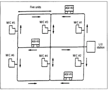
station Figure 1

Schematic View of Hypothetical FMS Under Study

fixed time interval rescheduling policy the degree of responsiveness would be higher with a tight buffer capacity schedule than the one with a loose buffer capacity. To avoid this interaction, the rescheduling points are determined as a function of total processing time of all jobs, which is the same regardless of the level of a scheduling factor.

Ten levels of scheduling frequency are used in the experiments: 0, 2, 4, 6, 8, 10, 12, 14, 16, 1000. Here, 4 means that the schedule is revised approximately four times during the makespan of the schedule. To reschedule the entire system at each machine breakdown event, a relatively large number (1000) is used. In other words, 1000 represents the case where the number of scheduling points is equal to the number of machine breakdowns. Note that level zero corre- sponds to the no rescheduling case (or fixed

sequencing) in which a schedule is generated once and never updated except for time shifting of operation start times. Thus, these two cases (no response vs. response to every unexpected interruption or event) represent two extreme policies.

System Considerations and

Experimental Conditions

Figure 1 shows the layout of the hypothetical

FMS studied in this paper, which was also used by the authors in a previous study. 2s There are six machines that can perform a wide variety of operations. Each machine can handle at most one operation at a time and has a limited input/output buffer in which parts can wait before and after an operation. Preemption is not allowed and setup times are

(5)

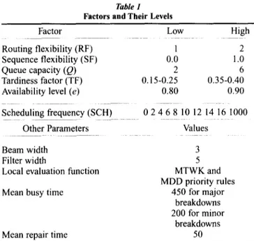
Table 1

Factors and Their Levels

Routing flexibility (RF) 1 Sequence flexibility (SF) 0.0 Queue capacity (Q) 2 Tardiness factor (TF) 0.15-0.25 Availability level (e) 0.80

Factor Low High 2 1.0 6 0.35-0.40 0.90 Scheduling frequency (SCH) 0 2 4 6 8 10 12 14 16 1000

Other Parameters Values Beam width

Filter width

Local evaluation function Mean busy time

Mean repair time

3 5 MTWK and MDD priority rules 450 for major breakdowns 200 for minor breakdowns 50

included in the operation time. The number of operations per part is either five or six with equal probability. Operation times are drawn from a 2-Erlang distribution. In addition, there is a load/unload (L/U) station (or input/output carousel) in the system. It is also used as a central buffer area to avoid blockings. Parts are transferred by three AGVs in the system.

This study considers the following factors: rescheduling frequency, buffer capacity, routing flexibility, and sequence flexibility. Table 1 provides the summa- ry of these factors and their levels. Both makespan and mean tardiness are used as performance criteria. The routing flexibility (RF) measure is taken from Chang, Matsuo, and Sullivan, 12 who define it in terms of the average number of machines on which a particular operation can be processed. Sequence flexibility (SF) is an indicator of precedence relationships between operations of the job. It measures the density of arcs on an acylic precedence graph. This measure is adapt- ed from Rachamadugu, Nandkeolyar, and Schreiber) 6 In the experiments, SF is set to 0 and 1 for low and high sequence flexibilities, respectively. Due dates are based on the total work content (TWK) rule. They are assigned such that the tardiness factor (TF) is approximately 20% and 40% for loose and tight due dates, respectively. In data sets, coefficient of variation of due dates ranges from 0.28 to 0.37 depending on the seed being used.

Machine breakdowns are modeled by the busy- time approach, 27 in which a random uptime is generated from a busy time distribution. The machine operates until its total accumulated busy (process-

ing) time reaches the end of this uptime. At that time, it fails for a random down time, after which an uptime is again generated. In the absence of real data, Law and Kelton 27 recommend a gamma distribution with shape parameter of 0.7 and scale parameter to be specified. They also propose a relationship between scale parameters and mean busy and down times, by which the model for machine breakdowns can be completely specified. In this framework, the level of machine breakdowns is measured by availability (or efficiency) level (that is, the long run ratio of a machine's busy time to busy plus downtime). In the experiments, 90% availability is used with 180 minutes of mean busy time and 20 minutes of mean down time. Hence, on average, 50 breakdowns occur during the scheduling horizon. The system is also simulated at the same availability level with less frequent machine breakdowns with longer repair times. In this case, 450 minutes of mean busy time and 50 minutes of down time are used. To achieve the 80% availability, mean busy time and downtime are set to 200 and 50 minutes, respectively.

Ten simulation replications are taken at each factor combination. Because there is a full-factor- ial experimental design, both levels (0.0 and 1.0) of precedence graph densities with the two levels of routing flexibility are used. In each replication, the problem data are generated using the experimental conditions specified above. It was tried for the same problem data to be used for each scheduling frequency level to measure the effect clearly. The algorithm develops a schedule for these ran- domly generated 25-job problems (approximately 135 operations on average). The resulting schedule is implemented via simulation until the next scheduling point. At that point, a new schedule is generated for all unprocessed operations and the process is continued. Hence, the simulation run length is equal to the makespan of the realized schedules. The parameters of the algorithm are given in the earlier study. 2s In terms of dispatching rules, 28,29 MTWK (most total work) and MDD (modified due date) are used for the makespan and mean tardiness measures, respectively.

Computational Results

In this section, the scheduling algorithm and the dispatching rules are used to examine frequency of

(6)

Journal o['Manu[acturing Systems Vol. 18/No. 4 1999

Table 2

Performances of Algorithm at Varying Levels of Scheduling Frequency

Experimental Settings 0 e=90%, 2136 ~t=450 116 sec

Performance o f Algorithm at Various Levels o f Scheduling Frequency Dispatch

Rules e=90%, 2086 g=200 114 sec 2 4 6 8 10 12 14 16 1000 Makespan Measure 2061 2020 1973 1940 1927 1904 1891 1886 1838 1983 (3.5%) (5.4%) (7.6%) (9.2%) (9.8%) (10.9%) (11.4%) (11.7%) (13.9°/,,) (7.2%)

130 sec 148 sec 172 sec 205 sec 208 sec 227 sec 235 sec 242 sec 387 sec 2.18 sec

e=80%, 2488

~=200

116 sec

2005 1939 1918 1880 1874 1871 1854 1856 1842 2009

(3.9%) (7.0%) (8.0%) (9.9%) (10.2%) (10.3%) (11.1%) (11.0%) (11.7%) (3.7%)

e=70%, 3115 ~=200 174 sec e=90%, 351 g=450 164 sec 2384 2370 2303 2269 2252 2238 2207 2201 2117 2190 (4.2%) (4.7%) (7.4%) (8.8%) (9.5%) (10.0%) (11.3%) (11.5%) (14.9%) (12.0%)

e=90%, 305

g=200

159 sec

2987 2970 2930 2850 2846 2757 2707 2704 2524 2570

(4.1%) (4.6%) (5.9%) (8.5%) (8.6%) (11.5%) (13.0%) (13.2%) (18.9%) (17.5%)

192 sec 223 sec 274 sec 307 sec 355 sec 375 sec 426 sec 450 sec 1031 sec 2.78 sec Mean Tardiness Measure

337 303 286 248 243 222 218 205 195 419

(4.0%) (13.6%) (18.5%) (29.3%) (30.7%) (36.7%) (37.9%) (41.6%) (44.4%) (-19.4%)

288 251 233 212 211 200 199 193 193 421

(5.5%) (17.7%) (23.6%) (30.5%) (30.8%) (34.4%) (34.7%) (36.7%) (36.7%) (-38.0)

511 501 473 434 419 410 393 348 571

10.6%) (11.3%) (16.3%) (23.2%) (25.9%) (27.4%) (30.4%) (38.4%) (-1.06%)

179 sec 203 sec 224 sec 251 sec 291 sec 303 sec 338 sec 784 sec 2.(15 sec

e=80%, 565 545

~=200 (3,5%)

163 sec 171 sec

969 917 902 858 819 771 733 707 599 845

(3.0%) (8.1%) (10.4%) (14.0%) (17.9%) (22.7%) (26.6%) (29.2%) (40.0%) (-15.3)

e=70%, 998

la=200

161 sec

e=availability level; g= mean busy time

scheduling and its relationships with other sched- uling factors (such as queue capacity, due-date tightness, sequence flexibility, and routing flexi- bility) in an FMS environment. The analysis is also done for different availability levels and busy time durations. As discussed in the previous section, a number o f test problems are used in the experi- ments. Ten replications are taken; that is, 10 ran- domly generated problems are used for factor combinations. The ANOVA test is performed for each scheduling criterion to test the significance o f the main factors and higher order interactions. The Bonferroni method is also applied to rank the levels o f some scheduling factors. Overall results o f the experiments are given in Table 2. In this

table, the first row for each experimental setting (that is, availability level and mean busy time duration) presents the results for makespan or mean tardiness measures. The second row presents the percentage improvement of the algorithm for each performance measure over the fixed sequencing policy at various scheduling frequencies. The third row gives computational times o f the algorithm and dispatching rules in CPU seconds.

In general, system performance deteriorates as the availability level decreases (that is, as the machines become less reliable). Longer mean duration of breakdowns (mean busy time = 450) for the same availability level (80%) has more negative effects on the system performance than the shorter

(7)

duration (mean busy time = 200). This means that there is a more severe impact on sytem performance from major machine breakdowns than from frequent minor breakdowns with quick repair times. Hence, prospective reactive scheduling systems should be designed in such a way that they can handle major interruptions even though the probability of these events is relatively low.

The results also indicate that thefixed sequencing approach is not an appropriate policy because there is always improvement in the performance measure as scheduling frequency increases (see the percent improvement numbers in parentheses with respect to the fixed sequencing). This means that it is not a good policy at all to generate a full schedule in advance and let the system recover from the effects of interruptions by following the events in a fixed sequence. As seen in Figure 2, which displays the ratio of the off-line algorithm to dispatching at various scheduling frequency levels, fixed sequencing is even worse than the dispatching policy for makespan. In the tardiness case, the MDD dispatching rule starts performing better than fixed sequencing only when the availability level drops below 80%. The above finding has an important practical implication because for those practitioners who would not like to exercise frequent rescheduling, it may be more suitable to employ a simple dispatching rule rather than an optimum-seeking scheduling algorithm. Besides, the computational time saving by dispatching can be very significant (Figures 2c and 2d). This also means that when system reliabili- ty is poor, there is more benefit in improving relia- bility than in the application of sophisticated scheduling techniques.

It is also observed that the other extreme policy (that is, reacting to every interruption in the system) does not seem to be an appropriate policy either. With such a continuous review policy, the marginal performance improvement (see Table 2, column 11 corresponding to 1000) is significantly smaller than that of the lower scheduling frequencies (see columns 7-10). The computational requirement of the scheduling algorithm is also extremely high at this level of scheduling frequency (Figures 2c and 2d).

From Table 2, it is clear that the system performance improves continuously as scheduling frequency increases. However, there is a diminishing rate of improvement with a dramatic increase in computation time as the revisions become more fre-

quent. These results are consistent with Church and Uzsoy's 7 study on the single-machine scheduling problem with the Lma~ objective. Therefore, a moderate level of scheduling frequency (for example, SCH = 10) is suggested to alleviate the negative effects of machine breakdowns without having too much computational burden.

Another observation is that employing more frequent rescheduling does not totally eliminate the negative effects of machine breakdowns either. In other words, rescheduling can help only to some extent in restoring the system operation back to the desired level. For example, as seen in Table 2, a 10% decrease in the availability level from e = 90% to e = 80% caus- es the performance of the fixed sequencing to deterio- rate about 19% (from 2086 to 2488), while the most frequent scheduling provides an improvement of 14% (from 2488 to 2117). Further reduction in the availability level from e = 80% to e = 70% results in even more deterioration in the performance (such as 25%), while the improvement by the highest level of rescheduling level is only 13%. The above observation is even more apparent in the tardiness case where the deterioration in the tardiness is about 78-85%, while the improvement due to frequent rescheduling is in the order of 35%. Hence, it may be more important to eliminate sources of variability and uncertainty in the system (such as breakdowns) than to eliminate their negative effects on the system performance by rescheduling. A similar observation is also made by Lawrence and Sewell, ~4 who state that whenever uncertainty is high it is of no use to try to improve the schedule generation algorithm, but reducing the variability of the system brings the real improvement.

The ANOVA test also confirms the results reported above (see Table 3). In general, the effects of all the main factors are found significant for each performance measure. Specifically, increasing the values of routing flexibility, sequence flexibility, buffer capacity, and scheduling frequency improve the system performance. These results are consistent with those of Sabuncuoglu and Karabuk. 25

Examining the effects of the scheduling frequency and its relationships with other factors reveals that differences between the algorithm and the dispatching rules decrease as the resource availability level decreases. This is partly due to the fact that the potential advantage of the optimum-seeking algorithm over these simple rules diminishes as the system experiences more interruptions in terms of machine break-

(8)

Journal (?['Manu[i~cturing Systems ~,bl. 18/No. 4 1999 == =S o .o # 1.3 1.2 1.1 1 0.9 0.8 07 0.6 05 04 0.3 = = 0.91450 ~ J 0.9/200 0--0 0.8/200 0.7/200 b ~ :~ + '8 ~o 1'2

~4 ~6

tboo Scheduling frequency (SCH) (a) Makespan performances

1.3 1.2 1.1 1 == ;~ 0.9

g

~ 0.8 o ~ 0.7 0.6 0.5 0.4 0.3 = 0.91450 t . 0.91200 _°° I~ 2' z~ 6' 8 1'0 12 1~, 16 1()00 Scheduling frequency (SCH)

(b) Mean tardiness performances

400 400 [ : :." 0.91450 = ×0.9/450 I 0.9•200 ~ 0.91200 / 0.8•200 ~ 0.8•200 / 7 - ~ 0.71200 ~7--.,-~ 0.7/2011 300 l 300 I ==

f_

o 200 = [

/

r j ~ lOO 0 , I O 2 4 ; ; 1'0 1)1'4 1'6 1;00 '0 i '4 6 '8 10 12 14 16 1000

Scheduling frequency (SCH) Scheduling frequency (SCH) (c) Makespan performances (d) Mean tardiness performances

Figure 2

Ratio of Algorithm to Dispatching at Various Scheduling Requency Levels

downs. These results are consistent with those of Yamamoto and Nof. z Although it is not explicitly stat- ed in their paper, the makespan difference between the optimum-seeking scheduling algorithm and the dis- patching rules seems to decrease as the number of machine breakdowns increases. Finally, it is noted that differences between the performance of the algorithm and the dispatching rules become more significant as

the system resources get tighter (that is, Q is smaller, but RF and SF are higher). This indicates that the off- line scheduling algorithm uses the system resources and flexibility more effectively.

Further analyses of the above findings reveal the fact that the basic assumptions (static and determin- istic assumptions) of scheduling algorithms such as those used in this paper are violated as the number

(9)

Performance Measure Makespan Tardiness

Table 3

Changes in Makespan and Tardiness for All Main Factors

(Arrows indicate the direction of change in performance measure value over factor levels)

2600 2500

RF SF Q TF e SCH

Low High Low High Low High Low High Low High 0 ... 1000

,•

= :: o_ LOOSE (200) I O_ TIGHT (200) 0---~0_ LOOSE (450) - O) 2400 2300 2200 2100 2000 1900 1800 1700 1600

~ ~ '8 '1o ~2 '14 '16~ooo

Scheduling frequency (SCH) (a) Makespan performances

c 500 400 300 200 100 : ~ o. LOOSE (200) ! Q_ TIGHT (200) o---oo_ LOOSE (450) - O ) () 2 '4 '6 '8 '10 '12 '14 ' 16 '1000 Scheduling frequency (SCH)

(b) Mean tardiness performances Figure 3

Interactions Between Scheduling Frequency and Buffer Capacity

of machine breakdowns increases. This behavior is especially observed in the makespan case, in which simple rules become highly competitive with the optimum-seeking algorithm as the availability level decreases. This is probably due to the fact that the algorithm generates schedules that are so compact that they are more sensitive (or fragile) to external changes than they are to the simple rules.

Although the algorithm uses more global information than the rules, this information becomes obsolete at a faster rate as the machine breakdown rate increases. In contrast, myopic rules, which use the most recent information to make local decisions, are less affected by the possible changes in the environment.

This paper also examines the interactions between scheduling frequency and other scheduling factors. Figure 3 illustrates frequency of scheduling vs. buffer capacity for makespan and mean tardiness. The results are presented for both la = 450 (major breakdowns with low probability of occur-

rence) and ~ = 200 (minor breakdowns with high occurrence rate).

As seen in this figure, the effect of rescheduling is high when buffer capacity is low. It seems that the system absorbs the negative impact of breakdowns with extra buffer capacities. For example, in the tight due date with ~t = 200 case, the improvement in tardiness is between 33% and 41% when moving from SCH = 0 (fixed sequencing) to SCH = 5 (moderate level) and SCH = 1000 (continuous scheduling). On the other hand, the improvement is between 24% and 27% for the same range of rescheduling frequency in the loose queue capacity case. Similar observations are made for the makespan measure, although the percentage of improvement is relatively smaller in this case. This study also indicates that coordination and integration of machines and AGVs are more important at the low buffer capacities, as the system becomes more sensitive to these unexpected events. Examining the interaction between scheduling frequency (SCH) and rout-

(10)

.hmrnal ~?f Manulbcturing 5~vstems Vol. 18/No. 4 1999 2400 2300 2200 2100 2000 1900 1800 1700 1600 z × RF_LOW(200) <~, d RF HIGH (200) O. 0 RF-LOW (450)

o l

O 2 4 6 8 10 12 14 16 1000 Scheduling frequency (SCH) (a) SCH with RF for the makespan measure

500 400 :~ 300 200 100

~

' ~ ~ HF_LOW (200) J RF HIGH (200) RFLOW (450) RF HIGH (450) 0 2 4 6 8 10 12 14 16 1000 Scheduling frequency (SCH)

(b) SCH with RF for mean tardiness measure

Figure 4

Interactions Between Scheduling Frequency and Flexibilities

ing flexibility (RF) reveals that SCH is more effective when RF is low compared to the high-RF case

(Figures 4a

and

4b).

This kind of counterintuitive result does not mean that the off-line scheduling algorithm cannot utilize routing flexibility effectively, but that the optimum-seeking methods generate more robust (or less fragile) schedules under the presence of RF by achieving uniform loads across the machines. In the low-RF case, the machine load balance is not maintained due to the lack of alternative machines. Hence, the schedules can easily be invalidated in highly loaded systems due to even minor machine breakdowns. For that reason, frequent rescheduling helps to improve system performance more than it does in the low-RF case. From the above discussion, one would infer that RF acts as a protective mechanism that absorbs the negative impact of interruptions on the system performance. Compared to RF, sequence flexibility (SF) does not seem to have a strong interaction with SCH, although it has a significant effect on performance measures. This is probably because SF does not alter the distribution of machine loads as much as RF; it only changes the sequence of operations of the jobs. The need for more frequent rescheduling remains

the same irrespective of the level of SE

Similarly, the interaction between SCH and TF is not a strong one. It is only observed for ~t = 450, where more frequent scheduling improves the mean

tardiness when TF is tight or more jobs are expected to be tardy. This means that the role of rescheduling for system performance is also important even when due dates are loose.

The sensitivity of results to processing time variation (PV) was also tested. In practice, processing times used in scheduling algorithms or other decision-making mechanisms are estimated by engi- neers, foremen, and so on. Unfortunately, these estimated quantities are subject to error due to stochastic variations in machining conditions, worker performance, and other conditions. The resulting differences between planned and actual processing times affect the schedules being implemented. Unlike machine breakdowns, these variations do not instan- taneously interrupt the system operation, but rather their effects accumulate over time and degrade the quality of the schedule. To model this situation, the processing times are perturbed when the schedule is realized on the shop floor. The estimated processing times used in the scheduling algorithm and the rules are still drawn from a 2-Erlang distribution. Actual processing times differ from the estimates by a certain amount when the schedule is implemented via the simulation model. Specifically, actual times are generated from a truncated normal distribution with mean equal to the estimated processing time and a certain coefficient of variation. During simulation

(11)

Table 4

Effects of Processing Time Variability and Machine Breakdowns for Makespan Availability e = 100% PV=0% PV=10% PV=20% 1994 204l 2281 2310 1517 1562 1696 1719 1403 1405 1875 1819 1247 1272 1360 1367 e-90% 2269 2528 F_low Algorithm 1988 Q=2 Dispatch 2312 F_low Algorithm 1474 Q=6 Dispatch 1689 F_high Algorithm 1434 Q=2 Dispatch 1896 F_high Algorithm 1217 Q=6 Dispatch 1378 F_low Algorithm 2283 Q=2 Dispatch 2570 Availability F_low Algorithm 1828 Q=6 Dispatch 1874 PV=30% 2101 2328 1605 1751 1459 1879 1292 1416 F_high Algorithm 1708 Q=2 Dispatch 2059 2311 2416 2531 2590 1863 1874 1928 1890 1898 1962 1693 1717 1750 2041 2141 2054 F_high Algorithm 1504 1521 Q=6 Dispatch 1575 1566 Availability e=80% F_low Algorithm 2679 2763 Q=2 Dispatch 2735 2765 F_low Algorithm 2189 2157 Q=6 Dispatch 2201 2234 F_high Algorithm 1967 1962 Q=2 Dispatch 2222 2214 1550 1553 1570 1574 2748 2772 2717 2783 2236 2295 2254 2307 2022 2016 2295 2301 1784 1818 1787 1822 F_high Algorithm 1770 1776 Q=6 Dispatch 1778 1780

experiments, three levels o f processing time variations were considered, corresponding to the coefficient o f variations o f 0.1, 0.2, and 0.3, respectively.

The effects o f P V were tested under various experimental conditions fqr makespan and mean tardiness criteria (see Tables 4 and 5). To save computation time, only two levels o f flexibility were included: low and high mean RF and SF set at low and high levels, respectively. Although the results were obtained for each level o f scheduling frequency, the best o f the scheduling/rescheduling approach was compared to the dispatching rules.

To understand the relationships between machine breakdown and P V better, several levels o f availabil-

ity were included in the experiments. The results for the makespan criterion indicate the performance o f both scheduling algorithms and dispatching rules are affected more by machine breakdowns than by PV. This is probably because, unlike machine breakdowns, PV does not immediately interrupt the system operation, but rather its effect is accumulated over time. For example, the average makespan performance o f the algorithm degrades by about 19% as a result o f a 10% reduction in the availability (from e = 100 to 90), whereas the effect is less than 1% for

10% processing time variation (Figure 5a).

It is also noted that dispatching rules are more robust to PV than the scheduling algorithm. This is

(12)

Journal o/ Manu['acturing 5~stems Vol. 18/No. 4 1999

Table 5

Effects of Processing Time Variability and Machine Breakdowns for Mean Tardiness F_low Algorithm Q=2 Dispatch F_low Algorithm Q=6 Dispatch F_high Algorithm Q=2 Dispatch F_high Algorithm Q=6 Dispatch F_low Algorithm Q-2 Dispatch F_low Algorithm Q=6 Dispatch F_high Algorithm Q=2 Dispatch Fhigh Algorithm Q=6 Dispatch Flow Algorithm Q=2 Dispatch F_low Algorithm Q=6 Dispatch F_high Algorithm Q=2 Dispatch F_high Algorithm Q=6 Dispatch Availability e=lO0% PV=0% PV=IO% PV=20% PV=30% 313 463 465 536 690 665 691 711 165 184 217 257 301 302 295 311 32 62 92 142 430 435 415 416 22 27 40 59 175 176 165 176 Availability e=90% 537 578 570 604 901 879 888 907 334 345 351 366 445 449 453 459 165 167 172 185 607 580 597 581 133 133 137 144 290 266 272 272 Availability e=80% 784 805 796 834 1081 ll01 1146 1125 537 542 556 565 631 634 645 652 296 305 315 327 729 739 743 752 285 283 282 295 435 421 423 423

probably because optimum-seeking methods are based on processing times. Consequently, any varia- tions in processing times can eliminate the potential benefits of these off-line schedules. This behavior is observed even if the schedules are revised frequent- ly. Nevertheless, in the dispatching case, the effect o f PV is minimal. It is also noted that the sampling errors in the simulation experiments are very low. For example, the standard error is only 15.54 for a makespan o f 1217 obtained for low flexibility and low queue capacity. On the other hand, in the pres- ence o f machine breakdowns and high processing time variability, the standard error increases to 19.70 for an average makespan value o f 2300.

Another observation is that the difference between the scheduling/rescheduling approach and dispatching policy decreases as availability decreas-

es and PV increases. As seen in

Figure 6,

the aver- age performance improvement o f the algorithm over dispatching is lowest when e = 80% and PV = 30%. The only exception is observed when the flexibility is high and queue capacity is low. This situation aris- es because the algorithm uses the flexibility more effectively and the rules do not have enough oppor- tunity to improve the system performance when there are two or fewer jobs in the queues. In other cases, PV combined with machine breakdowns affects the performance of the scheduling algorithm so badly that the potential benefits of using an opti- mum-seeking, off-line scheduling method diminish, but it still yields 30% better performance than the dispatching policy.

Similar observations are also made for the mean tardiness measure

(Table 5, Figures 5

and 6). Again,

(13)

2350 2200 2050 1900 1750 1600 1450 I

: = Breakdown level (AIg) PVlevel(AIg) t---E1Breakdown level (Disp)

~

O---O~level(Disp)

Z;

750 650 55o I =~ 45O :~ 350 250 150 50

/

1300' 0 I'0 10 0 10 20

Percentage of changes (%) Percentage of changes (%) (a) Makespan vs. percentage of changes (b) Mean tardiness vs. percentage of changes

I

- × Breakdown level (AIg) i PVlevel(AIg) E ~ 3 Breakdown level (Disp) '3"~OPVlevel(Disp)

Figure 5

Performance of Algorithm for Percentage Changes of Availability Level and Processing Time Variation (PV) Level

80 80 70 6O z= E o 50 '5 40 3O e = 100% e = 90% e = 80% 2 0 10 0 70 6O "~ 40 e~

~

3o 20 10 e = 100% e = 90% .~ ~ e = 80%

\,

0 10 20 30 0 10 20 30

Processing time variation Processing time variation (a) Makespan case (b) Tardiness case

Figure 6

Average Performance Improvement of Algorithm over Dispatching for Processing Time Variation (PV) Levels

the effect of machine breakdowns on the system performance is more than that of PV. From the performances of the algorithm and the dispatching rules, it seems that the system absorbs the negative impact of machine breakdowns and PV easily when queue capacity is high and flexibility is high. As in the makespan case, the dispatching rules are less sensitive to processing time variation. The scheduling algorithm seems to be more affected by PV due to the same reasons explained above. Nevertheless, the differences between these two scheduling approach-

es (off-line represented by the beam search based algorithm and on-line represented by the dispatching rule) are significant under every condition tested.

Concluding Remarks and

Recommendations for

Further Research

In this paper, scheduling/rescheduling approaches have been studied in an FMS environment. Several reactive scheduling policies have also been tested

(14)

,h)urnal o['Manu['acturing Systems

Vol. 18/No. 4 1999

under various operating conditions. The results are summarized as follows.

First, it is not always beneficial to reschedule the operations in response to every machine breakdown, because the potential benefits o f more frequent scheduling are marginal after a certain number revi- sions. Instead, a periodic response with an appropri- ate period length would be sufficient to cope with these interruptions.

Second, scheduling frequency has significant inter- actions with routing and sequence flexibility. In gener- al, the effect of scheduling frequency increases as the level of flexibility is reduced, possibly because the higher level of flexibility compensates for the negative impact of interruptions. Scheduling frequency has greater effect on the performance measures as system resources and due dates become tighter.

Third, machine breakdowns have more negative impact on the system performance than do process- ing time variations. This is probably because machine breakdowns have an immediate impact on the system, whereas the effect of PV on the system performance is accumulated over time.

Fourth, the dispatching rules are more robust to PV than the scheduling algorithm because schedules generated by off-line algorithms are based on pro- cessing times, and any deviation from these esti- mates can affect the resulting schedules.

Fifth, when the system experiences frequent machine breakdowns and higher PV, differences between the two scheduling approaches decrease. This observation clearly confirms the intuition that the potential benefit of optimum-seeking algorithms (or off-line scheduling approach) in real manufacturing environments may not be as good as expected because of the dynamic nature of such systems.

The results presented in this paper should be interpreted with reference to the assumptions and experimental conditions described earlier. There is a definite need for further research to test the policies under different conditions. One such condition is the dynamic and stochastic environment in which more realistic comparisons can be made (such as model- ing dynamic job arrivals in longer time horizons and considering other stochastic events like due-date changes, rework, and so on). Another research topic, as often practiced by some AI researchers (for exam- ple, see Zweben et al.3°), is to find efficient ways to repair the existing schedule rather than generating it from scratch.

References

1. J. Hutchison, K. Leong, D. Synder, and E Ward, "ScheduLing Approaches for Random Job Shop Flexible Manufacturing Systems," lnt 7 Journal o f Production Research (v29, 1991 ), pp1053-1067.

2. M. Yamamoto and S.Y. Nor, "Scheduling/Rescheduling in the

Manufacturing Operating System Environment," lnt'l Journal ~/' Production Research (v23, 1985), pp705-722.

3. R.T. Nelson, C.A. Holloway, and R.M. Wong, "Centralized Scheduling and Priority Implementation Heuristics for a Dynamic Job Shop Model with Due Dates and Variable Processing Times," AIIE Trans. (vl9, 1977), pp95-102.

4. A.R Muhleman, A.G. Lockett, and C.K. Farm "'Job Shop Scheduling Heuristics and Frequency of Scheduling," lnt 7 .hmrnal ~?[' Production Research (v20, 1982), pp227-241.

5. J.C. Bean, J. Birge, J. Mintenhal, and C. Noon, "Matchup Scheduling

with Multiple Resources, Release Dates, and Disruptions," Operations Research (v39, 1991 ), pp470-483.

6. D. Wu, R.H. Storer, and R Chang, "One-Machine Rescheduling Heuristics with Efficiency and Stability as Criteria," Computers & Operations Research (v20, 1993), pp I - 13.

7. L. Church and R. Uzsoy, "Analysis of Periodic and Event-Driven Rescheduling Policies in Dynamic Shops," lnt 7 ,hmrnal 0[" Computer Integrated Mfg. (v5, 1992), pp 153-163.

8. I.M. Ovacik and R. Uzsoy, "'Rolling Horizon Algorithms for a Single Machine Dynamic Scheduling Problem with Sequence-Dependent Set-Up Times," lnt 7 Journal ~ f Production Research (v32, 1994), pp 1243-1263.

9. V.J. Leon, S.D. Wu, and R.H. Storer, "Robustness Measures and Robust Scheduling for Job Shops," liE Trans. (v26, 1994), pp32-43. 10. R.L. Daniels and P Kouvelis, "Robust Scheduling to Hedge Against Processing Time Uncertainty in Single-Stage Production," Mgmt. Science (v41, 1995), pp363-376.

11. S.'~ Mehta and R. Uzsoy, "Predictable Scheduling of a Job Shop Subject to Breakdowns," IEEE Trans. on Robotics and Automation (v14,

1988), pp365-378.

12. Y.L. Chang, H. Matsuo, and R. Sullivan, "'A Bottleneck-Based Beam Search for Job Scheduling in a Flexible Manufacturing System," htt 7 Journal o f Production Research (v27, 1989), pp 1949-1963.

13. N. Raman, EB. Talbot, and R. Rachamadugu, "Due Date Based Scheduling in a General Flexible Manufacturing System 2' .lournal ~?[' Operations Mgmt. (v8, 1989), pp115-132.

14. M. Shaw, S. Park, and N. Raman, "'Intelligent Scheduling with

Machine Learning Capabilities: The Induction of Scheduling Knowledge," liE Trans. (v24, 1992), pp156-168.

15. K.N. McKay, J.A. Buzacott, and R.E Safayeni, The Scheduler,s" Knowledge ~[' UneertainO': The Missing Link in Knowledge Based Production Management Systems (Elsevier Science Publishers B.V., 1989), pp171-189.

16. A. Dutta, "'Reacting to Scheduling Exceptions in FMS Environments," liE Trans. (v22, 1994), pp300-314.

17. M.S. Fox and S.E Smith, "ISIS-Knowledge Based System for Factory Scheduling," Expert Sw~tems (vl, 1984), pp25-49.

18, S.E Smith, P Ow, J. Potvin, N. Muscettola, and Matthys, "'An Integrated Framework for Generating and Revising Factory Schedules," Journal (~[ Operational Research Socie O, (v4 I, 1990), pp539-552.

19. S. Smith, "OPIS: A Methodology and Architecture for Reactive Scheduling," in Intelligent Scheduling, M. Zweben and M. Fox, cds. (San Francisco: Morgan Kaufmann Publishers, 1994), pp29-56.

20. E. Szelke and R. Kerr, "Knowledge-based Reactive Scheduling," Production Planning and Control (v5, 1994), pp 124-145.

21. M. Kim and 5(. Kim, "Simulation Based Real-time Scheduling in a Flexible Manufacturing System," Journal ~?['MJg. Systems (v13, n2, 1994), pp85-93.

22. E. Kutanoglu and I. Sabuncuoglu, "Experimental Investigation of Scheduling Rules in a Dynamic Job Shop with Weighted Tardiness Costs,'" 3rd Industrial Engg. Research Conf., 1994, pp656-661.

23. Y. He, M. Smith, and R. Dudek, "Effects of Inaccuracy of Processing Time Estimation on Effectiveness of Dispatch Rules," 3rd Industrial Engg. Research Conf., 1994, pp308-313.

(15)

24. S.R. Lawrence and E.C. Sewell, "Heuristic, Optimal, Static, and Dynamic Schedules when Processing Times are Uncertain," Journal of Operations Mgmt. (v15, 1997), pp71-82.

25. I. Sabuncuoglu and S. Karabuk, "A Beam-Search Based Algorithm and Evaluation of Scheduling Approaches," liE Trans. on Scheduling and Logistics (v30, 1998), pp179-191.

26. R. Rachamadugu, U. Nandkeolyar, and q2J. Schreiber, "Scheduling with Sequence Flexibility," Decision Science (v24, 1993), pp315-241.

27. A. Law and W.D. Kelton, Simulation Modeling and Analysis" (New

York: McGraw-Hill, 1992).

28. I. Sabuncuoglu and D.L. Hommertzheim, "Experimental Investigation of FMS Due-date Scheduling Problem: Evaluation of Machine and AGV Scheduling Rules," Int7 Journal of Flexible Mfg. Systems (v5, 1993), pp301-324.

29. I. Sabuncuoglu, "A Study of Scheduling Rules ofFMSs: A Simulation Approach," lnt 7 Journal of Production Research (v36, 1998), pp527-546.

30. M. Zweben, B. Daun, E. Davis, and M. Deale, "Scheduling and Rescheduling with Iterative Repair," in Intelligent Scheduling, M. Zweben

and M. Fox, eds. (San Francisco: Morgan Kaufmann Publishers, 1994), pp241-255.

Appendix (The Beam Search Based

Scheduling Algorithm)

Notation X,Y

f

b N Bk v(PS)

set of partial AGV-machine schedules filterwidth parameter

beamwidth parameter

total number of machine operations partial schedule k E 1 ... b

an upper bound value for partial schedule PS (or value of solution when PS is complete) The Algorithm Initialize Bk k E 1 ... b n+-I while n! = N n~--n + 1 foreach Bk X+-- generate(Bk) Y~--- filter(X,J) For each y E Y v(y)¢-- evaluate(y) y * ~ min{v(y)/y E Y} Bk~-- Bk ~ y* end for endwhile B* = min{v(B,)lk ~ 1 ... b}

The procedure generate(.) takes a partial schedule

PS as input and generates all the possible AGV- machine scheduling decision pairs based on the system state described by PS. The details of this procedure are described below. Procedure filter(.) reduces

the cardinality o f X t o f u s i n g simple rules; that is, it selects a subset of X that will be input to a more thorough evaluation by the procedure evaluate(.).

After the application of procedure evaluate(.), the

most promising node is selected and added to the partial schedule associated with that particular Bk.

At any level of the search tree, there are b partial schedules that the algorithm keeps. After the tree is exhausted, the BI with the best schedule value is

selected to be the final solution. In the beam search based algorithm, the filter procedure uses dispatch rules, and the evaluation algorithm tentatively con- structs a full schedule beginning from Bk and measures its objective value.

Additional notation for procedure generate(PS)

i

J

m g G dij,,,,g Pi, m,g Stij, m Sid, m,g f i~,nl,g PS U(PS) subscript of jobs subscript of operations subscript of machines subscript of AGVs set of AGVs

earliest time AGV g delivers job i to machine m for itsjth operation

earliest time AGV g loads job i from machine m

earliest start time o f j t h operation of job i on machine m

earliest start time of operationj of job i on machine m if the job is transported by AGV g earliest finish time of operation j of job i on machine m if the job is handled by AGV g a partial AGV-machine schedule

a set of operations to be scheduled immediately after a given partial schedule PS,

(16)

Journal o[ Manu['acturing Systems Vol. 18/No. 4 1999

U(PS) = {nln=(i,j,m,s')},

where each element n is defined by the jth operation of job i on machine m to start processing at time s'

D(PS)

a set of scheduling decisions for a given

PS

after AGV considerations,

D(PS) =

{nln=(ij, m,s',g,p,d, sJ)},

where each element n defines scheduling of AGV g to pick up job i at time p, deliver it to machine m at time d, and scheduling of machine m to start processing thejth operation of job i at time s and finish it at time f Note that

D(PS)

has four additional terms due to AGV considerations, when compared with

U(PS).

procedure

generate(PS)

Step 1.

Step 2.

Step 3.

Step 4.

Step 5.

Determine the elements of

U(PS)

by considering routing and sequence flexibilities and buffer space constraints.

For each combination of

n E U(PS)

and g E G, compute

(p,d, sJ)

values and form the elements

of D(PS).

For each g E G select an element of

D(PS)

with d = min{du, m,~r}. If there are other elements of

D(PS)

such that the scheduling decision associated with those selected elements can be implemented without increasing their p values, delete these elements. Group the elements of

D(PS)

according to the same

(i,j,m)

values. In each group, keep the element that satisfies min{d~j,,.,g - s'ij,,,,0} and delete others. Break ties in favor of the one with the least p/,,.,g value. Group the elements of

D(PS)

according to the same i values. In each group, keep the one with the smallest

fj,,,,g

and delete others. Break ties arbitrarily.

Step 6.

Compute earliest finish time, j * = min~j,m,g} over the elements of

D(PS).

Delete the elements with

Sij, m,~ >.~.

The first step integrates routing and sequencing decisions. Sequence flexibility and buffer space availability are also considered at this stage. In Step 2, AGV alternatives are determined for each schedulable operation in

U(PS).

A new set,

D(PS),

is formed after AGV considerations. Step 3 ensures that all AGV schedules are active (that is, an AGV cannot meet the transportation requirements of other jobs without violating the feasibility of the AGV schedule). Step 4 reduces the number of AGV alternatives for each schedulable machine operation to one. Later in Step 5, the number of alternatives for each job (due to routing and sequence flexibilities) is reduced to one. Finally, active machine schedules are formed in Step 6.

Authors' Biographies

Ihsan Sabuncuoglu is an associate professor of industrial engineering at Bilkent University. He received his BS and MS degrees in industrial engineering from Middle East Technical University and his PhD in industrial engineering from Wichita State University. Dr. Sabuncuoglu teaches and conducts research in the areas of simulation, scheduling, and manufacturing systems. He has published papers in liE Transactions, the International Journal of Production Research, the International Journal of Flexible Manufacturing Systems, the International Journal o[" Computer Integrated Manufacturing, Computers and Operations Research, the European Journal of Operational Research, Production Planning and Control, the Journal of Operational Research Society, (2)mputers and Industrial Engineering, the International Journal of Management Science-OMEGA, and the Journal of Intelligent Manufacturing. He is on the editorial board of the International Journal of Operations and Quantitative Management. He is an associate member of IIE and the Institute for Operations Research and the Management Sciences.

Suleyman Karabuk is a PhD student in industrial engineering at Lehigh University. He received his BS degree in industrial engineering from Middle East Technical University and MS degree in industrial engineering from Bilkent University. His research interests include scheduling, stochastic programming, and distributed decision making.