An operator theoretic approach to robust control of infinite dimensional systems

SURVEY

AN OPERATOR THEORETIC APPROACH TO ROBUST CONTROL OF

INFINITE DIMENSIONAL SYSTEMS

HITAY ¨OZBAY1

Abstract. The purpose of this paper is to give an overview of the skew Toeplitz approach to H∞ _{control of a class of infinite dimensional systems. Numerical steps involved in the} computations of optimal and suboptimal controllers are demonstrated with different examples, including flexible beam models and systems with time delays.

Keywords: distributed parameter systems, time delay, robust control, skew-Toeplitz operators. AMS Subject Classification: 93C05, 93C80, 93B28, 93B36, 93B35.

1. Introduction

This paper provides an overview of the so-called skew Toeplitz approach to H

∞

control of

a class of infinite dimensional systems, [45]. The author has given invited presentations on

this topic at various scientific meetings, such as 17th International Symposium on Mathematical

Theory of Networks and Systems (MTNS 2006) Kyoto, Japan, and 2nd International Conference

on Control and Optimization with Industrial Applications (COIA 2008) Baku, Azerbaijan. The

present paper is a brief summary of these presentations.

It is now well-known that robust controllers, under the presence of unstructured L

∞

_-norm

bounded perturbations in the plant transfer matrix, can be obtained from an H

∞

_{optimization,}

[168]. Many different approaches have been developed for H

∞

_{control of finite dimensional}

systems, and computational tools are now widely available, [32, 34, 47, 54, 56, 84], [94, 124,

137, 155, 172, 173]. Robust control under `

1

optimality, and other types of uncertainty, are also

studied widely, see [9, 12, 28, 148] and their references. For time delay systems (an important

class of infinite dimensional systems), H

∞

_{controllers started to appear in the literature in}

the mid 1980s, [41, 46, 174]. Over the last 20 years there has been significant progress in the

extension of these first results to larger classes of infinite dimensional systems, see e.g. [5, 24,

25, 31, 43, 53, 57, 58, 71, 75, 78, 86, 93], [107, 111, 112, 118, 119, 129, 130, 135, 140, 144, 151].

One of the methods used in the computation of H

∞

_{controllers for infinite dimensional systems}

is the “skew Toeplitz” approach, [45]. The importance of skew Toeplitz operators in H

∞

_control

has been noticed by Foias, Tannenbaum and their collaborators, and this term first appears in

[11]. In this approach H

∞

optimal and suboptimal controllers are directly computed without

approximating the plant.

For infinite dimensional systems robust controllers can also be obtained by approximating the

plant and then using standard techniques developed for the control of finite dimensional systems,

1_{Department of Electrical and Electronics Engineering, Bilkent University, Ankara, Turkey,} e-mail: hitay@bilkent.edu.tr

Manuscript received November 2012.

by keeping track of the original approximation error, see e.g. [6, 23, 76, 87, 88, 104, 105, 120, 133]

and their references. See [22] for an early review of H

∞

_{control of distributed parameter systems}

in general, [154] for state-space approach to H

∞

_{control of such systems, and [100, 157] for}

reviews of state-space and operator theoretic approaches to H

∞

control of time delay systems.

For time delay systems, and some other classes of distributed parameter systems, H

∞

_controllers

can also be derived from a game theoretic approach, [10, 139]. For the most recent results on

H

∞

_{control of systems with input-output delays, see [98, 171] and their references. Repetitive}

control design, [68], under certain performance and robustness conditions, can be posed as a

robust control problem for systems with time delays, [63, 123, 142, 158]. Sampled-data controller

design, with certain types of optimality conditions result in an H

∞

_{control problem for time delay}

systems, see [8, 20, 67, 160] for further references. Robust stability of time delay systems (within,

and outside, the framework of H

∞

control) is widely studied, [19, 33, 49, 50, 59, 64, 70, 74, 81, 83],

[85, 89, 109, 110, 102, 121, 122, 146, 147, 153]. Several issues related to robust control of fractional

delay systems has been considered in [14]. Stability robustness against small time delays have

been considered for various types of plants, see e.g. [17, 90, 97, 103] and their references.

Flexible structure models which include internal time delays, are considered in [65, 66]. For

spatially invariant distributed parameter systems, [7], H

∞

_{optimal controllers are obtained from}

a parameterized family of finite dimensional problems; see also [27]. Robust control of infinite

dimensional systems is also covered in the book [26].

In Section 2 some key results from operator theory are reviewed and their link with the H

∞

control are shown. In Section 3 numerical computations of optimal and suboptimal controllers

are demonstrated based on the formulae derived in [60, 149]. Plants considered in Section 3 are

systems with time delays, [39, 61], and an infinite dimensional flexible beam model, [87, 88].

2. H

∞

Control problems

In this section some important results from operator theory are reviewed and a short

descrip-tion of the of the skew Toeplitz approach is given to illustrate the technique used in finding

optimal and suboptimal H

∞

_{controllers. An excellent background material can be found in a}

recently published book [161].

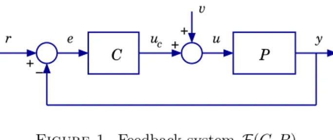
The standard feedback system F(C, P ) is shown in Figure 1, where C is the controller to be

designed and P is the plant to be controlled. The systems P and C are assumed to be linear

operators on appropriately defined function (signal) spaces. For simplicity of the presentation,

all systems considered are single input single output unless otherwise stated.

P

c u

C

v − + + + y u e r

Figure 1. Feedback system F(C, P )

We say that a linear time invariant system whose input output behavior is characterized by

the transfer function H(s) is said to be stable if H ∈ H

∞

_{(see [26, 139, 175] for a discussion on}

the transfer functions of infinite dimensional systems, here we assume that the transfer function

is the “quotient of the Laplace transform of the output and input, with initial condition zero”).

The feedback system F(C, P ) is stable if and only if S = (1 + P C)

−1

_{, P S and CS are in H}

∞

_.

Here S is the sensitivity function. The set of all controllers stabilizing this feedback system for

a given P is denoted by C(P ).

Most important features of the H

∞

_{control problems are captured by the weighted sensitivity}

minimization problem, which is to find

γ

o

=

inf

C∈C(P )

kW (1 + P C)

−1

_k

∞

(1)

and the corresponding optimal controller C

o

∈ C(P ), for a given plant P and a weight W ;

typi-cally W, W

−1

∈ H

∞

. There are several approaches to this problem depending on the structure

of the problem data.

First, let us assume that W is infinite dimensional (an irrational transfer function) and P is

finite dimensional (a rational transfer function). We can solve this problem using

Nevanlinna-Pick interpolation, as follows. For simplicity of the exposition assume that z

1

, . . . , z

nz

are the

zeros and p

₁

, . . . , p

_np

are the poles of P in C

₊

, and P has no poles or zeros on the imaginary

axis. In this case, C ∈ C(P ) is equivalent to having the sensitivity function S = (1 + P C)

−1

in H

∞

_{, with S(z}

i

) = 1 and S(p

j

) = 0. Then, γ

o

is the smallest γ > 0 such that there exists a

function F ∈ H

∞

_{such that}

kF k

∞

≤ 1 and F (z

i

) = γ

−1

W (z

i

), F (p

j

) = 0

for i = 1, . . . , n

_z

, j = 1, . . . , n

_p

. This is the Nevanlinna-Pick interpolation problem, and can be

solved from the problem data W and P , see [44, 45, 82, 170]. Once γ

o

and the corresponding

optimal F is computed, the resulting controller is C = (γ

−1

_{W − F )/P F . Note that in this}

case the problem solution depends on W (z

_i

), and W (s) can be irrational. In summary, when

the plant is finite dimensional and the weight is infinite dimensional, the weighted sensitivity

minimization problem can be solved using Nevanlinna-Pick interpolation.

Clearly, we cannot use this approach when the plant P is infinite dimensional (with infinitely

many C

+

zeros or poles). For such plants we will assume that W is finite dimensional and use the

characterization of C(P ) given below. First, assume that P can be written as P (s) = N (s)/D(s)

with N, D ∈ H

∞

such that there exist X, Y ∈ H

∞

satisfying

X(s)N (s) + Y (s)D(s) = 1.

Then the set of all controllers stabilizing F(C, P ) is (see e.g. [3, 138, 165] and their references)

C(P ) =

½

X + DQ

Y − N Q

: Q ∈ H

∞

_{, Y − N Q 6= 0}

¾

.

Let us now assume that the plant has finitely many unstable modes, i.e. D(s) can be taken as

a rational function. In this case X(s) should be chosen in such a way that

Y (s) =

1 − X(s)N (s)

D(s)

∈ H

∞

_.

Clearly, using Lagrange interpolation one can find a rational X(s) satisfying the above

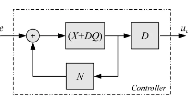
require-ment. Note also that stabilizing controllers are in the form

C =

D(X + DQ)

1 − N (X + DQ)

(2)

and they can be implemented as shown in Figure 2.

In particular, when the plant is stable we can choose N = P , D = 1 and X = 0. This leads

to

γ

o

= inf

Figure 2. Stabilizing Controller

The next crucial step is to perform inner outer factorization of the plant:

P = M

n

N

o

where M

n

is inner and N

o

is outer.

Defining Q

1

= W N

o

Q (we assume that W N

o

is invertible in H

∞

; otherwise, see the discussion

in [40, 48] on the absorption of the outer factor), we have

γ

_o

=

inf

Q1∈H∞

kW − M

_n

Q

₁

k

_∞

.

(3)

The problem (3) can be put into the framework of the Nehari problem, [108], and that gives

γ

o

= kΓk,

where Γ is the Hankel operator whose symbol is M

∗

n

W ∈ L

∞

. We will assume that the norm

is achieved on the discrete spectrum, i.e., kΓk > kΓk

e

, the essential norm (see [45, 169] for the

computation of the essential norm). In this case γ

o

and the corresponding optimal Q

1

∈ H

∞

,

and hence the optimal controller C ∈ C(P ), can be obtained by computing the largest singular

value, and the corresponding singular vector of Γ, see also [2] for the characterization of all

suboptimal solutions of this problem. For more details see [45].

The problem (3) can also be solved using Sarason’s Theorem, [134], or the Commutant Lifting

Theorem, [44, 143], as follows. Let us map the right half plane, C

+

, to the unit disc, D, via the

conformal map z = ϕ(s) =

s−1_s+1

, s = ϕ

−1

_{(z) =}

1+z

1−z

. Define functions w(z) = W (ϕ

−1

(z)) and

m

n

(z) = M

n

(ϕ

−1

(z)). For the inner function m := m

n

define H(m) = H

2

(D) ª mH

2

(D). When

m is rational (finite Blaschke product), the space H(m) is finite dimensional, otherwise it is

infi-nite dimensional. Let S be the unit shift operator on `

2

, i.e. it can be seen as the multiplication

by z on H

₂

(D). Then the compressed shift operator T is defined as T = Π

_H(m)

S|

_H(m)

, where

Π

_H(m)

denotes the orthogonal projection onto H(m). Now the solution of (3) is

γ

o

= kw(T)k.

Since w(z) is rational, it can be written as w(z) = b(z)/a(z). Under the assumption γ

o

>

kw(T)k

_e

, (the norm is strictly greater than the essential norm), γ

_o

is the largest γ for which

there exists a non-zero f ∈ H(m) such that

0 =

¡

b(T)

∗

b(T) − γ

2

a(T)

∗

a(T)

¢

f =: A

γ

f .

(4)

The operator A

γ

is called a skew Toeplitz operator, and γ

o

is the largest γ which makes A

γ

singular; the optimal Q

1

∈ H

∞

, and hence the optimal controller C ∈ C(P ), are determined

from the corresponding f ∈ H(m) as

w − m

n

q

opt1

=

b(T)f

a(T)f

.

(5)

A closer examination of (4) leads to a finite set of linear equations for the existence of a non-zero

f ∈ H(m), even when H(m) is infinite dimensional. This set of linear equations determine γ

o

and the corresponding f . Then the optimal controller is obtained from (5) using this f . For

complete details and further references see [45].

The weighted sensitivity minimization is known as a one-block H

∞

_{control problem. An}

extension of this problem, which also takes into account robust stability of the feedback system,

[32], is the mixed sensitivity optimization: find

γ

o

=

inf

C∈C(P )

°

°

°

°

·

W

1

(1 + P C)

−1

W

2

P C(1 + P C)

−1

¸°

_°

°

°

∞

(6)

and the corresponding optimal controller. Again, using the parameterization (2), we transform

the problem (6) into a problem of finding

γ

o

= inf

Q∈H∞

°

°

°

°

·

W

1

(1 − N (X + DQ))

W

₂

N (X + DQ)

¸°

°

°

°

∞

and the corresponding optimal Q ∈ H

∞

_{. After a series of inner-outer factorizations, [47], the}

above problem is further reduced to finding smallest γ such that there exists Q

1

∈ H

∞

satisfying

°

°

°

°

·

W − M Q

₁

G

¸°

_°

°

°

∞

≤ γ label2bl

1

(7)

where W, G, M, Q

1

are determined from the problem data W

1

, W

2

, N, D. In particular Q

1

is

determined from Q by an invertible relation, M is inner infinite dimensional, and G is finite

dimensional. If the plant is stable N = P and D = 1, then W is finite dimensional as well.

Otherwise, it has a special structure W = W

o

+ M

1

W

c

o

where W

o

, c

W

o

are finite dimensional and

M

₁

is the infinite dimensional part of M , i.e., M = M

₁

M

₂

with M

₂

being finite dimensional

(assuming that the plant has finitely many unstable modes). Next step is to do a spectral

factorization:

F

_γ∗

F

γ

= γ

2

− G

∗

G.

That transforms (??) into a problem of finding smallest γ such that

kW F

_γ−1

− M Q

₂

k

_∞

≤ 1,

(8)

where Q

2

= Q

1

F

γ−1

. Clearly, now the problem (8) is in the form (3), and the approach outlined

earlier is applicable. The problem (??) is a two-block H

∞

_{control problem, and as we have seen}

above, it can be reduced to a one-block problem by a spectral factorization.

One step extension of the two-block problem is the four-block problem. That also can be

reduced to a one-block problem by a series of spectral factorizations, see e.g. [47]. The key

observation we make in this context is that when the weights are finite dimensional, and the

inner-outer factorizations of the plant have already been made (see below for examples), we only

need to do spectral factorizations for finite dimensional systems, see [45, 80] for further details.

In general, there are several technical difficulties in performing spectral factorizations for infinite

dimensional systems, [159].

The problem of robust stabilization in the gap metric can be posed as a special case of

the mixed sensitivity minimization, (6), with special weights W

1

and W

2

. This problem has

been studied for various classes of infinite dimensional systems, see e.g. [35, 53, 150] and their

references. The uncertainty model in this case is coprime factor perturbations. Briefly, if the

uncertain plant is given as

P

∆

=

N

_D

∆ ∆

=

N + ∆

N

D + ∆

_D

, N, D, ∆

N

, ∆

D

∈ H

with

N

∗

N + D

∗

D = 1 k

·

∆

_N

∆

D

¸

k

∞

< δ

then a controller C ∈ C(P ), where P = N/D, is also in C(P

_∆

) if and only if it satisfies

°

°

°

°D

−1

(1 + P C)

−1

·

1

C

¸°

_°

°

°

∞

≤

1

δ

.

(9)

For certain classes of infinite dimensional systems this type of uncertainty modeling is very

helpful in finding finite dimensional controllers. See for example [120] for robust controller design

for a thin airfoil where the D

∆

term contains an irrational transfer function (the Theodorsen’s

function) which is approximated by a second order rational function, [114].

It turns out that, see e.g. [51, 55, 156], minimizing the left hand side of (9) over all C ∈ C(P )

(for the largest allowable δ), is equivalent to finding the norm of a Hankel operator whose symbol

is [D

∗

_N

∗

_{]. Clearly, (9) is a special case of the two block problem, (6), (with W}

1

= D

o−1

, the

inverse of the outer part of D, and W

2

= N

o−1

), and it too reduces to a one block problem.

In summary, several different H

∞

_{control problems can be reduced to the generic form (3),}

which is solved via (5). Then the optimal controller is computed using the optimal Q ∈ H

∞

in

(2).

3. Optimal solution of the mixed sensitivity minimization problem

In this section we present a closed form solution for the mixed sensitivity problem (6), taken

from [149].

3.1. Examples of Plants Considered. The plants considered in [149] have the coprime

fac-torization in the form

P (s) =

M

n

(s)N

o

(s)

M

d

(s)

,

(10)

where M

n

is inner, N

o

is outer and M

d

is finite dimensional and inner. The formula given here

is also valid for certain different classes of infinite dimensional plants (including plants with

infinitely many C

+

poles) with some modifications, see [60, 61].

Examples of infinite dimensional plants in the form (10) are as follows.

1. A stable first order system with transport delay:

P

₁

(s) =

e

−hs

τ

p

s + 1

, h > 0, τ

_p

> 0.

M

d

(s) = 1, M

n

(s) = e

−hs

, N

o

(s) =

_τ

1

p

s + 1

.

2. An unstable system with transport delay:

P

₂

(s) = e

−hs

1

s − a

, h > 0, a > 0,

M

d

(s) =

s − a

_{s + a}

, M

n

(s) = e

−hs

, N

o

(s) =

_{s + a}

1

.

3. An unstable system with internal time delays:

P

3

(s) =

s + 3 + 2(s − 1)e

−0.4s

s

2

_{+ se}

−0.2s

_{+ 5e}

−0.5s

,

which can be re-written as

P

3

(s) =

P

_P

N

(s)

where

P

N

(s) =

s + 3 + 2(s − 1)e

−0.4s

(s + 1)

2

,

P

D

(s) =

s

2

_{+ se}

−0.2s

_{+ 5e}

−0.5s

(s + 1)

2

.

It can be shown that P

D

(s) has only two zeros in C

+

, these are the unstable poles of the plant,

p

₁

and p

₂

. On the other hand, P

_N

(s) has infinitely many zeros in C

₊

. Inner-outer factorization

of this plant can be done, [61], by finding p

1

, p

2

, and the single C

+

zero, z

1

, of

P

_N

(s) =

2(s + 1) + (s − 3)e

−0.4s

(s + 1)

2

.

At this point we should mention that there are several tools for finding the zeros of a

quasi-polynomial, see e.g. [36, 37, 38, 131] for the Matlab-based program DDE-BIFTOOL, and also

[29, 91, 113] for other techniques and further references on this topic. Now, the zeros of P

D

(s)

in C

₊

are computed as p

_1,2

≈ 0.467 ± j1.889, and the zero of P

_N

(s) in C

₊

is z

₁

≈ 0.247. We

define

M

d

(s) =

(s − p

₁

)(s − p

₂

)

(s + p

1

)(s + p

2

)

, M

1

(s) =

s − z

₁

s + z

1

.

Then, the plant P

₃

can be written in the form (10) with M

_d

as above and

M

n

(s) = M

1

(s)

s + 3 + 2(s − 1)e

−0.4s

2(s + 1) + (s − 3)e

−0.4s

,

N

o

(s) =

_M

P

N

(s)

1

(s)

M

d

(s)

P

_D

(s)

.

4. A flexible beam: Consider an Euler-Bernoulli beam having free ends with Kelvin-Voigt

damping. Assume that the beam length and all other parameters are normalized to unity,

except the damping constant ε > 0, [88]. Denote the deflection of the beam at time t and

location x along the elastic axis of the beam by w(x, t). Suppose that a transverse force, −u(t),

is applied at one end of the beam, e.g. at x = 1 (see Figure 3).

x=1 force input

u(t)

w(0,t)

x=0

Figure 3. Beam with free ends.

The beam dynamics are given by the following PDE, [16, 87],

∂

2

_w

∂t

2

+ ε

∂

5

_w

∂x

4

_∂t

+

∂

4

_w

∂x

4

= 0

(11)

with boundary conditions

∂

2

_w

∂x

2

(0, t) + ε

∂

3

_w

∂x

2

_∂t

(0, t) = 0,

∂

2

_w

∂x

2

(1, t) + ε

∂

3

_w

∂x

2

_∂t

(1, t) = 0,

∂

3

w

∂x

3

(0, t) + ε

∂

4

w

∂x

3

_∂t

(0, t) = 0,

∂

3

_w

∂x

3

(1, t) + ε

∂

4

_w

∂x

3

_∂t

(1, t) = u(t).

Let the output of the system be the acceleration at x = 0, i.e. y

o

(t) :=

∂

2

∂t2

w(0, t) and consider a

low-pass characteristics for the sensor dynamics: H(s) = e

−hs

_{/(1 + τ s), with h ≥ 0 and τ > 0.}

Define the output available for feedback as Y (s) = H(s)Y

_o

(s). Note that w(0, t) is the deflection

at the opposite end of the beam as the applied force −u(t), i.e., even if the sensing delay is zero

the plant is non-minimum phase due to non-collocated actuator and sensor. We will ignore the

actuator dynamics here. Transfer function of the plant (including the sensor dynamics) can be

derived as in [87]: P

4

(s) :=

Y (s)_{U (s)}

,

P

₄

(s) =

s

2

(sinh β − sin β) e

−hs

β

3

_{(cos β cosh β − 1)(1 + εs)(1 + τ s)}

,

(12)

where β

4

₌

−s2 (1+εs)

.

One can show that P

4

(s) can be expressed as infinite products of second order terms. These

product representations display its poles and zeros. It also facilitate inner/outer factorizations

which are essential for solving the H

∞

_{optimization problems.}

P

4

(s) =

2e

−hs

τ s + 1

∞

Y

n=1

g

n

(s),

(13)

where

g

n

(s) =

³

1 + εs −

_4αs24 n

´

³

1 + εs +

_φs24 n

´

for values of s where this infinite product converges. In [87] it is shown that (13) converge

everywhere in the closed right half plane and can be written as quotients of H

∞

_{functions. We}

factor P

4

= M

n

N

o

, where M

n

(s) = e

−hs

B(s),

N

o

(s) =

_{(τ s + 1)}

2

∞

Y

n=1

³

1 + s

q

ε

2

₊

1 α4 n

+

s2 4α4 n

´

³

1 + εs +

_φs24 n

´

,

(14)

B(s) =

∞

Y

n=1





2α

4 n

³

ε +

q

ε

2

₊

1 α4 n

´

− s

2α

4 n

³

ε +

q

ε

2

₊

1 α4 n

´

+ s



 .

(15)

It has been shown that [87, 88], N

o

(s) ∈ H

∞

and B(s) ∈ H

∞

converge in the closed right

half-plane. The zeros of P

₄

are at

s = 2α

4_n

Ã

ε ±

s

ε

2

₊

1

α

4 n

!

for n = 1, 2, ...,

(16)

where

cos(α

n

) sinh(α

n

) = sin(α

n

) cosh(α

n

), for α

n

> 0.

Also, P

4

has a singularity at −1/ε, and poles at

s =

−φ

4n

2

Ã

ε ±

s

ε

2

₋

4

φ

4 n

!

for n = 1, 2, ...,

where cos(φ

n

) cosh(φ

n

) = 1, for φ

n

> 0.

3.2. H

∞

_{Optimal Controller. Assume that the weights W}

1

and W

2

are rational and

(W

2

N

o

), (W

2

N

o

)

−1

∈ H

∞

, then optimal H

∞

controller for plant (10) can be written as, [149],

C

opt

= E

γo

(s)M

d

(s)

N

−1 o

(s)F

γo

(s)L(s)

1 + M

_n

(s)F

_γo

(s)L(s)

,

(17)

where E

_γ

(s) =

³

W1(−s)W1(s) γ2

− 1

´

, and for the definition of the other terms, let the right half

plane zeros of E

γ

(s) be β

i

, i = 1, . . . , n

1

, the right half plane poles of P (s) be α

k

, k = 1, . . . , `

and that of W

1

(−s) be η

i

i = 1, . . . , n

1

. Then,

F

γ

(s) = G

γ

(s)

n1

Y

i=1

s − η

i

s + η

i

,

where

G

∗_γ

G

γ

=

µ

1 −

µ

W

₂∗

W

2

γ

2

− 1

¶

E

γ

¶

₋₁

(18)

and G

γ

, G

−1γ

∈ H

∞

, and L(s) =

LL12(s)(s)

, L

1

and L

2

are polynomials with degrees ≤ (n

1

+ ` − 1)

and they are determined by the following interpolation conditions,

0 = L

1

(β

i

) + M

n

(β

i

)F

γ

(β

i

)L

2

(β

i

),

(19)

0 = L

2

(−β

i

) + M

n

(β

i

)F

γ

(β

i

)L

1

(−β

i

),

0 = L

1

(α

k

) + M

n

(α

k

)F

γ

(α

k

)L

2

(α

k

),

0 = L

2

(−α

k

) + M

n

(α

k

)F

γ

(α

k

)L

1

(−α

k

)

for i = 1, . . . , n

1

and k = 1, . . . , `. The optimal performance level, γ

o

, is the largest γ value

such that the spectral factorization (18) can be done and the interpolation conditions (19) are

satisfied for some non-zero L

1

, L

2

. A Matlab-based computer program is available for computing

γ

_o

and all the functions appearing in (17); it can be downloaded from the author’s web site:

http://www.ee.bilkent.edu.tr/~ozbay/HINFCON.rar

With respect to the above controller formula, first point to note is that the spectral

factor-ization in question is finite dimensional and the order of F

_γ

is at most the order of W

₁

plus the

order of W

2

. Secondly, L(s) is characterized by its 2(n

1

+ `) coefficients, and the interpolation

conditions (19) can be re-written as

R

γ

Φ = 0,

(20)

where the entries of the 2(n

1

+ `) × 1 vector Φ contain the coefficients of L

1

and L

2

, and the

2(n

1

+ `) × 2(n

1

+ `) matrix R

γ

is constructed from M

n

(s), F (s) and β

i

, α

k

, for i = 1, . . . , n

1

and

k = 1, . . . , `. Clearly, explicit computation of M

n

(s) is not necessary for the construction of R

γ

;

all we need is its values at β

i

’s and α

k

’s. See [42] for more detailed discussion of this point and

further references. Due to symmetry in the interpolation conditions, L(s) term in the optimal

controller satisfies |L(jω)| = 1, but it may or may not be stable. The final observation we make,

probably the most important one from the point of view of “controller implementation,” is that

the controller has internal unstable pole-zero cancelations: the C

+

zeros of E

γo

and M

d

are

canceled by the zeros of 1 + M

_n

(s)F

_γo

(s)L(s). Since M

_n

is infinite dimensional, e.g. time delay,

exact cancelation is not always possible. For this reason, these cancelations should be studied

in more detail and a new equivalent structure, which can be implemented in a stable manner,

should be investigated, see [61, 62] for a discussion of this problem within the framework of

general time delay systems.

Here we illustrate the optimal H

∞

_{controller for P}

1

, with the mixed sensitivity problem

weights

W

1

(s) =

1 + ²s

_{s + ²}

, W

2

(s) = k(1 + ατ

p

s).

In this case the plant is stable, so ` = 0, and W

1

is first order, so n

1

= 1, and thus n

1

+ ` − 1 = 0,

which means that L(s) is just a constant, +1 or −1. We have only one linear equation to form,

and that gives γ

o

. When we let ² → 0, we obtain γ

o

as the largest root of the equation

p

1 − (k/γ)

2

_{− kατ}

_p

_/γ

2

_{− sin(h/γ) = 0}

in the interval

2h_π

≤ γ < ∞. It can be shown that, [116, 141], the optimal H

∞

_{controller has an}

“internal model controller” structure

C

_opt

=

Q

opt

1 − P (s)Q

opt

, Q

_opt

=

Q

o

1 + F

o

Q

o

,

where

Q

o

(s) = k

1 + ατ

_γ

p

s

o

s

,

F

o

(s) =

_{1 + ατ}

1

p

s

F

1

(s) where F

1

(s) =

γ

o

s(sin(h/γ

o

) + γ

o

s cos(h/γ

o

)) + e

−hs

1 + (γ

o

s)

2

.

(21)

It should be noted that F

1

(s) in (21) is the transfer function of a linear time invariant system

whose impulse response is of finite duration, (it is non-zero only on the interval [0 , h]). Thus F

1

is a stable system. On the other hand, if F

1

(s) is implemented as in (21) by using γ

o

and h with

a slight uncertainty in these parameters, then stability of F

₁

can be lost. So, one must be careful

about the “fragility” of a particular controller implementation in this framework; this is a topic

discussed in detail in the literature [79]. If F

1

(s) is implemented by taking a stable approximation

(for example, approximation of its impulse response by another finite impulse response filter),

then this will lead to a small stable perturbation in the numerator and denominator coprime

factors of the controller, which will not cause any fragility problems as shown in [52, 95, 125].

4. Conclusions

The purpose of this paper was to introduce the readership of this mathematics journal to a

specific control engineering problem.

There are also very interesting applications of the theory given here to data flow control

in computer communication networks. Interested readers are referred to [106] [21, 69, 96],

[13, 15, 136], [126], [127], [152], for related issues and technical details related to this particular

application.

Another useful application of the theory presented here is in the suppression of cavity flow

oscillations in aerodynamics. Typically, this is an application involving nonlinear infinite

dimen-sional models, [1, 4, 18, 73, 77, 145]. Nevertheless, using simplified linear models H

∞

_controllers

can be designed for performance improvement, see e.g. [162, 163, 166, 167] and their references.

In particular [166] shows that in this application the plant and the weights are infinite

dimen-sional, but by exploiting the special structure of the plant and how the weights are defined, it

is possible to find a suboptimal H

∞

_{controller suppressing cavity flow oscillations.}

Recently, in [117] it has been shown that the set of equations (20) can be further simplified

and the size of the γ-dependent matrix whose singularity gives the optimum performance level

can be reduced to n

1

× n

1

, where n

1

is the order of the weight W

1

(s). For detailed discussion

References

[1] Aamo, O.M., Krsti´c, M., (2003), Flow Control by Feedback: Stabilization and Mixing, Springer-Verlag, London, 198p.

[2] Adamjan, V.M., Arov, D.Z., Krein, M.G., (1971), Analytic properties of Schmidt pairs for a Hankel operator and the generalized Shur–Takagi problem, Math. USSR Sbornik, 15, pp.31-73.

[3] Aliev, F.A., Larin, V.B., (1998), Optimization of Linear Control Systems: Analytical Methods and Compu-tational Algorithms, Gordon and Breach, Amsterdam, 272p.

[4] Atwell, J., Borggaard, J., King, B., (2001), Reduced order controllers for burgers’ equation with a nonlinear observer, Int. J. Appl. Math. Comput. Sci., 11, pp.1311-1330.

[5] Azuma, T., Sagara, S., Fujita, M., Uchida, K., (2003), Output feedback control synthesis for linear time-delay systems via infinite-dimensional LMI approach, Proc. of the 42nd IEEE Conference on Decision and Control, Maui, Hawaii, pp.4026-4031.

[6] Balas, M.J., (1988), Finite-dimensional controllers for linear distributed parameter systems: Exponential stability using residual mode filters, J. of Mathematical Analysis and Applications, 133, pp.283-296. [7] Bamieh, B., Paganini, F., Dahleh, M.A., (2002), Distributed control of spatially invariant systems, IEEE

Trans. Automatic Control, 47(7), pp.1091-1107.

[8] Bamieh, B., Pearson, J.B., (1992), A general framework for linear periodic systems with applications to H∞ sampled-data control, IEEE Trans. Automatic Control, 37, pp.418-435.

[9] Barmish B.R., (1994), New Tools for Robustness of Linear Systems, Macmillan, New York.

[10] Ba¸sar, T., Bernhard, P., (1995), H∞ _{Optimal Control and Related Minimax Design Problems: A Dynamic} Game Approach, 2nd Ed., Birkhauser, Boston.

[11] Bercovici, H., Foias, C., Tannenbaum, A., (1988), On skew Toeplitz operators, Operator Theory: Advances and Applications, 32, pp.21-43.

[12] Bhattacharyya, S.P., Chapellat, H., Keel, L.H., (1995), Robust Control: The Parametric Approach, Prentice-Hall, Upper Saddle River, NJ.

[13] Blanchini, F., Lo Cigno, R., Tempo, R., (1998), Control of ATM networks: fragility and robustness issues, Proc. of the 1998 American Control Conference, Philadelphia, PA, 5, pp.2847-2851.

[14] Bonnet, C., Partington, J.R., (2002), Analysis of fractional delay systems of retarded and neutral type, Automatica, 38(1), pp.1133-1138.

[15] Bonomi, F., Fendick, K. W., (1995), The rate-based flow control framework for the available bit rate ATM service, IEEE Network Magazine, 25, pp.24-39.

[16] Bontsema, J., Curtain, R.F., Schumacher, J.M., (1988), Robust Control of Flexible Structures: a case study, Automatica, 24(2), pp.177-186.

[17] Bontsema, J., De Vries, S.A., (1988), Robustness of flexible structures against small time delays, Proc. 27th IEEE Conf. on Decision and Control, pp.1647-1648.

[18] Burns, J.A., Singler, J., (2005), Feedback control of low dimensional models of transition to turbulence, Proc. of the 44th IEEE Conference on Decision and Control and the European Control, Seville, Spain, pp.3140-3145. [19] Cao, Y-Y., Lam, J., (2000), Robust H∞_{control of uncertain Markovian jump systems with time-delay, IEEE}

Trans. on Automatic Control, 45(1), pp.77-83.

[20] Chen, T., Francis, B.A.,(1996), H∞_{-optimal sampled-data control: Computation and designs, Automatica,} 32(2), pp.223-228.

[21] Cooke, K.L., Huang, W., (1996), On the problem of linearization for state-dependent delay differential equations, Proceedings of the American Mathematical Society, 124, pp.14171426.

[22] Curtain, R.F., (1990), H∞ _{control for distributed parameter systems: a survey, Proc. of the 29th CDC,} Honolulu, Hawaii, pp.22-26.

[23] Curtain, R.F., Glover, K., (1986), Robust stabilization of infinite dimensional systems by finite dimensional controllers, Systems and Control Letters, 7, pp.41-47.

[24] Curtain, R.F., Sasane, A.J., (2003), Hankel norm approximation for well-posed linear systems, Systems and Control Letters, 48, pp.407-414.

[25] Curtain, R.F., Zhou, Y., (1996), A weighted mixed-sensitivity H∞_{-control design for irrational transfer} matrices, IEEE Trans. on Automatic Control, 41(9), pp.1312-1321.

[26] Curtain, R.F., Zwart, H.J., (1995), An Introduction to Infinite-Dimensional Linear Systems Theory, Springer-Verlag, New York.

[27] D’Andrea, R., Dullerud, G.E., (2003), Distributed control design for spatially interconnected systems, IEEE Transactions on Automatic Control, 48(9), pp.1478-1495.

[28] Dahleh, M.A., Diaz-Bobillo, I.J., (1995), Control of Uncertain Systems: A Linear Programming Approach, Prentice-Hall, Englewood Cliffs, NJ.

[29] Datko, R., (2004), Empirical methods for determining the stability of certain linear delay systems, in advances in time-delay systems, S. Niculescu and K. Gu Eds., Springer-Verlag, Lecture Notes in Computational Science and Engineering, 38, pp.183-192.

[30] Di Bernardo, M., Garofalo, F., Manfredi, S., (2005), Performance of robust AQM controllers in multibot-tleneck scenarios, Proc. of the 44th IEEE Conference on Decision and Control and the European Control Conference, Seville, Spain.

[31] Djouadi, S.M., Birdwell, J.D., (2005), On the optimal two-block H∞ _{problem, Proc. of the 2005 American} Control Conference, Portland, OR, pp.4289-4294.

[32] Doyle, J.C., Francis, B.A., Tannenbaum, A., (1992), Feedback Control Theory, Macmillan Publishing Co., New York.

[33] Dugard, L., Verriest, E.I., Eds., (1998), Stability and Control of Time-Delay Systems, LNCIS, Springer-Verlag, London, 228p.

[34] Dullerud, G.E., Paganini, F., (2000), A Course in Robust Control Theory: A Convex Approach, Springer-Verlag, New York, 417p.

[35] Dym, H., Georgiou, T.T., Smith, M.C., (1993), Direct design of optimal controllers for delay systems, Proceedings of 32nd IEEE Conference on Decision and Control, San Antonio TX, pp.3821-3823.

[36] Engelborghs, K., Luzyanina, T., Samaey, G., (2001), DDE-BIFTOOL v. 2.00: a Matlab package for bifurca-tion analysis of delay differential equabifurca-tions, Report TW 330, Katholieke Univ. Leuven, October .

[37] Engelborghs, K., Roose, D., (2002), On stability of LMS methods and characteristic roots of delay differential equations, SIAM J.Numer.Anal., 40(2), pp.629-650.

[38] Engelborghs, K., Luzyanina, T., Roose, D., (2002), Numerical bifurcation analysis of delay differential equa-tions using DDE-BIFTOOL, ACM Transacequa-tions on Mathematical Software, 28(1), pp.1-21.

[39] Enns, D., ¨Ozbay, H., Tannenbaum, A., (1992), Abstract model and controller design for an unstable aircraft, AIAA Journal of Guidance Control and Dynamics, March-April, 15(2), pp.498-508.

[40] Flamm, D.S., (1992), Outer factor ‘Absorption’ for H∞ _{control problems, Int. J. Robust and Nonlinear} Control, 2(1), pp.31-48.

[41] Flamm, D.S., Mitter, S., (1987), H∞_{Sensitivity minimization for delay systems, Systems and Control Letters,} 9, pp.17-24.

[42] Flamm, D.S., Yang, H., Ren, Q., K. Klipec, (1991), Numerical computation of inner factors for distributed parameter systems, Proc. of the 29th Annual Allerton Conference on Communication, Control and Compu-tation, Monticello IL, pp.72-73.

[43] Flamm, D.S., Yang, H., (1994), Optimal mixed sensitivity for SISO distributed plants, IEEE Transactions on Automatic Control, 39(6), pp.1150-1165.

[44] Foias, C., Frazho, A.E., (1990), The Commutant Lifting Approach to Interpolation Problems, Birkh¨auser, Basel.

[45] Foias, C., ¨Ozbay, H., Tannenbaum, A., (1996), Robust Control of Infinite Dimensional Systems: Frequency Domain Methods, Lecture Notes in Control and Information Sciences, 209, Springer-Verlag, London. [46] Foias, C., Tannenbaum, A., Zames, G., (1986) Weighted sensitivity minimization for delay systems, IEEE

Trans. Automatic Control, 31, pp. 763–766.

[47] Francis, B.A., (1987), A Course in H∞_{Control Theory, Lecture Notes in Control and Information Sciences,} 88, Springer Verlag, 156p.

[48] Francis, B.A., Zames, G., (1984), On H∞_{optimal sensitivity theory for SISO feedback systems, IEEE Trans.} Aut. Contr., 29(1), pp.9-16.

[49] Fridman, E., Pila, A., Shaked, U., (2003), Regional stabilization and H∞_{control of time-delay systems with} saturating actuators, Int. J. Robust and Nonlinear Control, 13(29), pp.885-907.

[50] Fu, M., Olbrot, A.W., Polis, M.P., (1989), Robust stability for time-delay systems: the edge theorem and graphical tests, IEEE Transactions on Automatic Control, 34, pp.813-820.

[51] Georgiou, T.T., Smith, M.C., (1990), Optimal robustness in the gap metric, IEEE Transactions on Automatic Control, 35(6), pp.673-686.

[52] Georgiou, T.T., Smith, M.C., (1990), Robust Control of Feedback Systems with Combined Plant and Con-troller Uncertainty, Proceedings of the American Control Conference, pp.2009-2013.

[53] Georgiou, T.T., Smith, M.C., (1992), Robust stabilization in the gap metric: controller design for distributed plants, IEEE Transactions on Automatic Control, 37, pp.1133-1143.

[54] Glad, T., Ljung, L., (2000), Control Theory: Multivariable and Nonlinear Methods, Taylor and Francis, London.

[55] Glover, K., McFarlane, D., (1989), Robust stabilization of normalized coprime factor plant descriptions with

H∞_{bounded uncertainty, IEEE Transactions on Automatic Control, 34, pp.821-830.}

[56] Green, M., Limebeer, D.J.N., (1995), Linear Robust Control, Prentice Hall, Englewood Cliffs.

[57] Gu, C., (1992), Eliminating the genericity conditions in the skew Toeplitz operator algorithm for H∞ opti-mization, SIAM J. Math. Anal., 23, pp.1623-1636.

[58] Gu, C., Toker, O., ¨Ozbay, H., (1996), On the two block H∞ _{problem for a class of unstable distributed} systems, Linear Algebra and its Applications, 234, pp.227-244.

[59] Gu, K., Kharitonov, V.L., Chen,J., (2003), Stability of Time-Delay Systems, Birkh¨auser, Boston.

[60] G¨um¨u¸ssoy, S., ¨Ozbay, H., (2004), On the Mixed Sensitivity Minimization for Systems with Infinitely Many Unstable Modes, Systems & Control Letters, 53(3-4), pp.211-216.

[61] G¨um¨u¸ssoy, S., ¨Ozbay, H., (2006), Remarks on H∞ _{Controller Design for SISO Plants with Time Delays,} Proc. of the 5th IFAC Symposium on Robust Control Design, Toulouse, France.

[62] Gumussoy, S., (2012), Coprime-inner/outer factorization of SISO time-delay systems and FIR structure of their optimal H∞ _{controllers, Int. J. Robust and Nonlinear Control, 22, pp.981998, DOI: 10.1002/rnc.1740.} [63] G¨uven¸c, L., (2001), Repetitive controller design in parameter space, Proc. of the 2001 American Control

Conference, Arlington, VA, June , pp.2749-2754.

[64] Gy¨ori, I., Hartung, F., Turi, J., (1998), Preservation of Stability in Delay Equations under Delay Perturba-tions, Journal of Mathematical Analysis and ApplicaPerturba-tions, 220(1), pp.290-312.

[65] Halevi, Y., (2002), On Control of Flexible Structures, Proc. of the 41st IEEE Conference on Decision and Control, Las Vegas, Nevada USA, December, pp.232-237.

[66] Halevi, Y., (2005), Control of Flexible Structures Governed by the Wave Equation Using Infinite Dimensional Transfer Functions, ASME Journal of Dynamic Systems, Measurement, and Control, 127, pp.579-588. [67] Hara, S., Yamamoto, Y., Fujioka, H., (1996), Modern and classical analysis/synthesis methods in

sampled-data control-a brief overview with numerical examples, Proc. of the 35th IEEE Conference on Decision and Control, Kobe Japan, pp.1251-1256.

[68] Hara, S., Yamamoto, Y., Omata, T., Nakano, M., (1988), Repetitive control systema new-type servo system, IEEE Trans. on Automatic Control, 33(11), pp.659-668.

[69] Hartung, F., Turi, J., (1997), On Differentiability of Solutions with Respect to Parameters in State-Dependent Delay Equations, Journal of Differential Equations, 135(2), pp.192-237.

[70] Haurania, A., Michalska, H.H., Boulet, B., (2003), Delay-dependent robust stabilization of uncertain neutral systems with saturating actuators, Proc. of 2003 American Control Conference, Denver, CO, pp.509-514. [71] Hirata, K., Yamamoto, Y., Tannenbaum, A., (2000), A Hamiltonian-based solution to the two block H∞

problem for general plants in H∞ _{and rational weights, Systems and Control Letters, 40, pp.83-95.}

[72] Hollot,C., Misra, V., Towsley, D., Gong, W., (2002), Analysis and design of controllers for AQM routers supporting TCP flows, IEEE Transactions on Automatic Control, 47(6), pp.945-959.

[73] Hristova, H., Etienne, S., Pelletier, D., Borggaard, J., (2006), A continuous sensitivity equation method for time-dependent incompressible laminar flows, Int. J. for Numerical Methods in Fluids, 50, pp.817-844. [74] Huang, Y-P., Zhou, K., (2000), Robust stability of uncertain time-delay systems, IEEE Trans. on Automatic

Control, 45(11), pp.2169-2173.

[75] Iftime, O., Kaashoek, M., Sasane, A., (2005) A Grassmannian band method approach to the NehariTakagi problem, J. Mathematical Analysis and Applications, 310(1), pp.97-115.

[76] Ito, K., Morris, K.A., (1998), An Approximation Theory of Solutions to Operator Riccati Equations for H∞ Control, SIAM J. Control and Optimization, 36(1), pp.82-99.

[77] Jovanovi´c, M.R., Bamieh, B., (2003), Frequency domain analysis of the linearized Navier-Stokes equations, Proc.of the 2003 American Control Conference, Denver, CO, pp.3190-3195.

[78] Kashima, K., ¨Ozbay, H., Yamamoto, Y., (2005), A Hamiltonian-based solution to the mixed sensitivity optimization problem for stable pseudorational plants, Systems and Control Letters, 54, pp.1063-1068. [79] Keel, L.H., Bhattacharyya, S.P., (1997), Robust, fragile, or optimal?, IEEE Transactions on Automatic

Control, 42(8), pp.1098-1105.

[80] Khargonekar, P.P., ¨Ozbay, H., Tannenbaum, A., (1989), The four block problem: stable plants and rational weights, International Journal of Control, 50, pp.1013-1023.

[81] Khargonekar, P.P., Poolla, K., (1986), Robust stabilization of distributed systems, Automatica, 22(1), pp.77-84.

[82] Khargonekar, P.P., Tannenbaum, A.,(1985), Noneuclidean metrics and the robust stabilization of systems with parameter uncertainty, IEEE Trans. Automatic Control, 30(10), pp.1005-1013.

[83] Kharitonov, V.L., (1999), Robust stability analysis of time delay systems: A survey, Annual Reviews in Control, 23(1), pp.185-196.

[84] Kimura, H., (1997), Chain-Scattering Approach to H∞_{Control, Birkhauser, Boston.}

[85] Kolmanovskii, V.B., Nosov, V.R., (1986), Stability of Functional Differential Equations, Academic Press, London.

[86] Le, D.K., Frazho, A.E., (1991), A numerical procedure for a non-rational H∞_{optimization problem in control} design, Systems & Control Letters, 16, pp.9-15.

[87] Lenz, K., ¨Ozbay, H., (1993), Analysis and robust control techniques for an ideal flexible beam, in Multidis-ciplinary Engineering Systems: Design and Optimization Techniques and their Applications, C.T. Leondes ed., Academic Press Inc., pp.369-421.

[88] Lenz, K., ¨Ozbay, H., Tannenbaum, A., Turi, J., Morton, B., (1991), Frequency domain analysis and robust control design for an ideal flexible beam, Automatica, 27, pp.947–961.

[89] Li, X., De Souza, C.E., (1997), Delay-dependent robust stability and stabilization of uncertainlinear delay systems: a linear matrix inequality approach, IEEE Trans. on Automatic Control, 42(8), pp.1144-1148. [90] Logemann, H., Rebarber, R., Weiss, G., (1996), Conditions for Robustness and Nonrobustness of the Stability

of Feedback Systems with Respect to Small Delays in the Feedback Loop, SIAM J. Control and Optimization, 34, pp.572-600.

[91] Louisell, J., (2004), Stability exponent and eigenvalue abscissas by way of the imaginary axis eigenvalues, in Advances in Time-Delay Systems, S. Niculescu and K. Gu Eds., Springer-Verlag, Lecture Notes in Compu-tational Science and Engineering, 38, pp.193-206.

[92] Low, S.H., Paganini, F., Doyle J.C., (2002), Internet congestion control, IEEE Control Systems Magazine, 22(1), pp.28-43.

[93] Lypchuk, T., Smith, M.C., Tannenbaum, A., (1988), Weighted sensitivity minimization: General plants in

H∞ _{and rational weights, Linear Algebra Appl., 109, pp.71-90.}

[94] Maciejowski, J.M., (1989), Multivariable Feedback Design, Addison Wesley, 424p.

[95] M¨akil¨a, P.M., (1998), Comments on ”Robust, fragile, or optimal?” IEEE Transactions on Automatic Control, 43, pp.1265–1267; DOI: 10.1109/9.718613

[96] Mallet-Paret, J., Nussbaum, R.D., (2003), Boundary layer phenomena for differential-delay equations withstate-dependent time lags: III, Journal of Differential Equations, 189, pp.640-692.

[97] Meinsma, G., Fu, M., Iwasaki, T., (1999), Robustness of the stability of feedback systems with respect to small time delays, Systems and Control Letters, 36(2), pp.131-134.

[98] Meinsma, G., Mirkin, L., (2005), H∞ _{Control of Systems With Multiple I/O Delays via Decomposition to} Adobe Problems, IEEE Trans. on Automatic Control, 50, pp.199-211.

[99] Meinsma, G., Zwart, H., (2000), On H∞ _{control for dead-time systems, IEEE Transactions on Automatic} Control, 45, pp.272-285.

[100] Mirkin, L., Tadmor, G., (2002), H∞_{Control of System with I/O Delay: A review of some problem-oriented} methods, IMA Journal of Mathematical Control and Information, 19(1-2), pp.185-199.

[101] Misra, V., Gong, W., Towsley, D., (2000), A fluid-based analysis of a network of AQM routers supporting TCP flows with an application to RED,in Proc. ACM SIGCOMM, Stockholm, Sweeden, Sep., pp. 151-160. [102] Morari, M., Zafiriou, E., (1989), Robust Process Control, Prentice Hall.

[103] Morg¨ul, ¨O, (1995), On the Stabilization and Stability Robustness Against Small Delays of Some Damped Wave Equations, IEEE Trans. Automatic Control, 40, pp.1626-1630.

[104] Morris, K.A., (1994), Convergence of Controllers Designed Using State-Space Techniques, IEEE Trans. Automatic Control, 39(10), pp.2100-2104.

[105] Morris, K.A., (2001), H∞_{-output feedback of infinite-dimensional systems via approximation, Systems &} Control Letters, 44(3), pp.211-217.

[106] Murray, R.M., Astrom, K.J., Boyd, S.P., Brockett, R.W., Stein, G.,(2003), Future directions in control in an information-rich world, IEEE Control Systems Magazine, 23(2), pp.20-33.

[107] Nagpal, K., Ravi, R., (1997), H∞_{control and estimation problems with delayed measurements: state space} solutions, SIAM J. Control and Optimization, 35(4), pp.1217-1243.

[109] Niculescu, S.-I., (2001), Delay Effects on Stability: A Robust Control Approach, LNCIS, 269, Springer-Verlag, .

[110] Niculescu, S-I., Dion, J-M., Dugard, L., (1996), Robust Stabilization for Uncertain Time-Delay Systems Containing Saturating Actuators, IEEE Trans. Automatic Control, 41, pp.742-747.

[111] Ohta, Y., (1999), Hankel Singular Values and Vectors of a Class of Infinite-Dimensional Systems: Ex-act Hamiltonian Formulas for Control and Approximation Problems, Mathematics of Control, Signals, and Systems, 12, pp.361-375.

[112] Ohta, Y., (2000), A study on the norm of mixed Hankel-Toeplitz operator, Proc. of the 2000 American Control Conference, Chicago, IL, June , pp.2765-2769.

[113] Olga¸c, N., Sipahi, R., (2004), A practical method for analyzing the stability of neutral type LTI-time delayed systems, Automatica, 40, pp.847-853.

[114] ¨Ozbay, H., (1993), Active control of a thin airfoil: flutter suppression and gust alleviation, Proc. of the 12th IFAC World Congress, Sydney, Australia, 2, pp.155-158.

[115] ¨Ozbay, H., (2000), Introduction to Feedback Control Theory, CRC Press LLC, Boca Raton, FL.

[116] ¨Ozbay, H., (2002), On the computation of H∞_{optimal controllers and connections with IMC-based design,} Applied and Computational Mathematics, 1(1), pp.5-13.

[117] ¨Ozbay, H., (2012), Computation of H∞ _{controllers for infinite dimensional plants using numerical linear} algebra, Numerical Linear Algebra With Applications, DOI: 10.1002/nla.1809.

[118] ¨Ozbay, H., Smith, M.C., Tannenbaum, A., (1993), Mixed sensitivity optimization for a class of unstable infinite dimensional systems, Linear Algebra and its Applications, 178, pp.43-83.

[119] ¨Ozbay, H., Tannenbaum, A., (1990), A skew Toeplitz approach to the H∞_{optimal control of multivariable} distributed systems, SIAM J. Control and Optimization, 28, pp.653-670.

[120] ¨Ozbay, H., Turi, J., (1994), On input/output stabilization of singular integrodifferential systems, Applied Mathematics and Optimization, 30, pp.21-49.

[121] Partington, J.R., Bonnet, C., (2004), H∞_{and BIBO stabilization of delay systems of neutral type, Systems} and Control Letters, 52, pp.283-288.

[122] Partington, J.R., Glover, K., (1990), Robust stabilization of delay systems by approximation of coprime factors, Systems & Control Letters, 14(4), pp.325-331.

[123] Peery, T.E. ¨Ozbay, H., (1997), H∞ _{optimal repetitive controller design for stable plants, Transactions of} the ASME Journal of Dynamic Systems, Measurement, and Control, 119, pp.541-547.

[124] Petersen, I.R., Ugrinovskii, V.A., Savkin, A.V., (2000), Robust Control Design Using H∞ _Methods, Springer-Verlag, London.

[125] Qiu, L., Davison, E.J., (1992), Feedback stability under simultaneous gap metric uncertainties in plant and controller, Systems and Control Letters, 18, pp.922.

[126] Quet, P-F., Ata¸slar, B., ˙Iftar, A., ¨Ozbay, H., Kalyanaraman, S., Kang, T., (2002), Rate-based flow con-trollers for communication networks in the presence of uncertain time-varying multiple time-delays, Auto-matica, 38, pp.917-928.

[127] Quet, P-F. ¨Ozbay, H., (2004), On the Design of AQM Supporting TCP Flows Using Robust Control Theory, IEEE Transactions on Automatic Control, 49(6), pp.1031-1036.

[128] Rebarber, R., Townley, S., Robustness with Respect to Delays for Exponential Stability of Distributed Parameter Systems, SIAM J. Control and Optimization, 37(1), pp.230-244.

[129] Rodriguez, A.A., Dahleh, M.A., (1990), Weighted H∞_{optimization for stable infinite dimensional systems} using finite dimensional techniques, Proc. of the 29th IEEE Conf. on Decision and Control, Honolulu HI, pp.1814-1819.

[130] Rodriguez, A.A., Dahleh, M.A., (1992), On the computation of induced norms for non-compact Hankel operators arising from distributed control problems, Systems and Control Letters, 19, pp.429-438.

[131] Roose, D., Luzyanina, T., Engelborghs, K., Michiels, W.,(2004), Software for stability and bifurcation analysis of delay differential equations and applications to stabilization, in Advances in Time-Delay Systems, S. Niculescu and K. Gu Eds., Springer-Verlag, Lecture Notes in Computational Science and Engineering, 38, pp.167-181.

[132] Rowley, C.W., Williams, D.R., Colonius, T., Murray, R.M. , MacMartin, D.G., Fabris, D., (2002), Model Based Control of Cavity Oscillations Part II: System Identification and Analysis, 40th Aerospace Sciences Meeting, January, Reno, NV, AIAA paper no. AIAA 2002-0972.

[133] Sano, H., (2002), Finite-dimensional H∞_{control of flexible beam equation systems, IMA Journal of} Math-ematical Control and Information, 19, pp.477-491.

[134] Sarason, D., (1967), Generalized interpolation in H∞_{, Transactions of the AMS, 127, pp.179-203.}

[135] Sasane, A., (2002), Hankel Norm Approximation for Infinite-Dimensional Systems, Springer-Verlag, Berlin. [136] S. Kalyanaraman, Jain, R., Fahmy, S., Goyal, R., Vandalore, B.,(2000), ERICA switch algorithm for ABR

traffic management in ATM networks, IEEE/ACM Transactions on Networking, 8, pp.87-98.

[137] Skogestad, S., Postlethwaite, I., (1996), Multivariable Feedback Control: Analysis and Design, John Wiley & Sons, Chicester, England.

[138] Smith, M.C., (1989), On stabilization and existence of coprime factorizations, IEEE Transactions on Auto-matic Control, 34(9), pp.1005-1007.

[139] Staffans, O.J., (1998), On the distributed stable full information H∞ _{minimax problem, Int. J. Robust} Nonlinear Control, 8, pp.1255-1305.

[140] Staffans, O.J., (2000), Well-Posed Linear Systems, Cambridge University Press.

[141] Starr, K.D., (2000), Infinite Dimensional Process Identification and H∞ _{Control Applied to an Internal} Model Controller, MS Thesis, The Ohio State University.

[142] Steinbuch, M., (2002), Repetitive control for systems with uncertain period-time, Automatica, 38(12), pp.2103-2109.

[143] Sz.-Nagy, B., Foias, C., (1970), Harmonic Analysis of Operators on Hilbert Space, North Holland, Amster-dam.

[144] Tadmor, G., (1997), Weighted sensitivity minimization in systems with a single input delay: A state space solution, SIAM J. Control and Optimization, 35(5), pp.1445-1469.

[145] Tadmor, G., Noack, B.R., (2004), Dynamic estimation for reduced Galerkin models of fluid flows, Proc.of the 2004 American Control Conference, Boston, MA, June-July, pp.746-751.

[146] Tarbouriech, S., J.M.G. da Silva Jr., (2000), Synthesis of Controllers for Continuous-Time Delay Systems with Saturating Controls via LMIs, IEEE Trans. Automatic Control, 45(1), pp.105-111.

[147] Tarbouriech, S., Peres, P.L.D., Garcia, G., Queinnec, I., (2000), Delay-dependent stabilization of time-delay systems with saturating actuators, Proc. of the 39th IEEE Conf. on Decision and Control, Sydney, Australia, December, pp.3248-3253.

[148] Tempo, R., Calafiore, G., Dabbene, F., (2005), Randomized Algorithms for Analysis and Control of Uncer-tain Systems, Springer-Verlag, London.

[149] Toker, O., ¨Ozbay, H., (1995), H∞_{Optimal and suboptimal controllers for infinite dimensional SISO plants,} IEEE Trans. Automatic Control, 40, pp.751-755.

[150] Toker, O., ¨Ozbay, H., (1995), Gap metric problem for MIMO delay systems: Parametrization of all subop-timal controllers, Automatica, 31(7), pp.931-940.

[151] Uchida, K., Ikeda, K., Azuma, T., Kojima, A., (2003), Finite-Dimensional Characterizations of H∞_Control for Linear Systems with Delays in Input and Output, Int. J. Robust and Nonlinear Control, 13(9), pp.833-843. [152] ¨Unal, H.U., Ata¸slar Ayyıldız, B., ˙Iftar, A., ¨Ozbay, H., (2006), Robust Controller Design for Multiple

Time-Delay Systems: The Case of Data-Communication Networks, Proc. of the MTNS2006, Kyoto, Japan. [153] Utkin, V., Guldner, J., Shi, J., (1999), Sliding Mode Control in Electromechanical Systems, Taylor and

Francis, London, 325p.

[154] Van Keulen, B., (1993), H∞ _{Control for Distributed Parameter Systems: A State-Space Approach,} Birkhauser, Boston.

[155] Vidyasagar, M., (1985), Control System Synthesis: A Factorization Approach, MIT Press, Cambridge MA, 436p.

[156] Vidyasagar, M., Kimura, H., (1986), Robust controllers for uncertain linear multivariable systems, Auto-matica, 22, pp.85-94.

[157] Watanabe, K., Nobuyama, E., Kojima, A., (1996), Recent Advances in Control of Time Delay Systems: A Tutorial Review, Proc. of the 35th IEEE Conf. on Decision and Control, Kobe, Japan, pp.2083-2089. [158] Weiss, G., H¨afele, M., (1999), Repetitive control of MIMO systems using H∞ _{design, Automatica, 35(7),}

pp.1185–1199.

[159] Winkin, J.J., Callier, F.M., Jacob, B., Partington, J.R., (2005), Spectral Factorization by Symmetric Ex-traction for Distributed Parameter Systems, SIAM J. Control and Optimization, 43(4), pp.1435-1466. [160] Yamamoto, Y., (1993), On the state space and frequency domain characterization of H∞_{norm, of}

sampled-data systems, Systems and Control Letters, 21 , pp.163-172.

[161] Yamamoto, Y., (2012), From Vector Spaces to Function Spaces: Introduction to Functional Analysis with Applications, SIAM, Philadelphia PA.