Shifting Network Tomography Toward A Practical Goal
Denisa Ghita, Can Karakus
∗, Katerina Argyraki, Patrick Thiran
EPFL, Switzerland
ABSTRACT
Boolean Inference makes it possible to observe the conges-tion status of end-to-end paths and infer, from that, the con-gestion status of individual network links. In principle, this can be a powerful monitoring tool, in scenarios where we want to monitor a network without having direct access to its links. We consider one such real scenario: a Tier-1 ISP operator wants to monitor the congestion status of its peers. We show that, in this scenario, Boolean Inference cannot be solved with enough accuracy to be useful; we do not at-tribute this to the limitations of particular algorithms, but to the fundamental difficulty of the Inference problem. In-stead, we argue that the “right” problem to solve, in this context, is compute the probability that each set of links is congested (as opposed to try to infer which particular links were congested when). Even though solving this problem yields less information than provided by Boolean Inference, we show that this information is more useful in practice, be-cause it can be obtained accurately under weaker assump-tions than typically required by Inference algorithms and more challenging network conditions (link correlations, non-stationary network dynamics, sparse topologies).
1. INTRODUCTION
Network performance tomography can be a powerful mon-itoring tool: it makes it possible to observe the status of end-to-end paths and infer, from that, the status of individual net-work links. The basic idea is to express the status of each ob-served path as a function of the status of the links that make up the path; in this way, we can form a system of equations, where the known entities are the path observations and the network topology, while the statuses of the links constitute the unknowns. The appeal of the approach is that it is ap-plicable in scenarios where one needs to monitor a network without having direct access to its links: a coalition of end-∗
Currently at Bilkent University,Turkey.
Permission to make digital or hard copies of all or part of this work for personal or classroom use is granted without fee provided that copies are not made or distributed for profit or commercial advantage and that copies bear this notice and the full citation on the first page. To copy otherwise, to republish, to post on servers or to redistribute to lists, requires prior specific permission and/or a fee.
ACM CoNEXT 2011, December 6–9 2011, Tokyo, Japan. Copyright 2011 ACM 978-1-4503-1041-3/11/0012 ...$10.00.
users could use network performance tomography to mon-itor the behavior and performance of their Internet Service Providers (ISPs); an ISP operator could use it to monitor the behavior and performance of its peers.
On the other hand, there are reasons to be skeptical about the applicability of this approach in practice. First, tomo-graphic algorithms necessarily make assumptions that can-not be verified in a real network (Sections 2 and 3), which means that their results may be inaccurate and, most impor-tantly, there is no way to tell to what extent they are inaccu-rate. Second, tomographic algorithms are typically designed and evaluated over generated graphs that model full router-level or Autonomous-System-router-level topologies; yet there is no evidence that these models capture well the topologies encountered in scenarios like the ones mentioned above, where using tomography would make sense—indeed, we will see that the topologies encountered in these scenarios can be sig-nificantly sparser (Section 3).
In this work, we look at whether and how network per-formance tomography could be useful in the following real scenario. A European Tier-1 ISP (we will call it the “source ISP”) wants to monitor the behavior and performance of its most “important” peers, i.e., the peers through which it routes most traffic that it cannot deliver directly to the cor-responding destination’s ISP. In particular, for each peer, the source ISP wants to understand: when the peer is responsi-ble for connectivity/performance proresponsi-blems encountered by the customers of the source ISP; how frequently the peer is congested and how its congestion level changes over the course of day or week; how well the peer reacts to excep-tional situations like Border Gateway Protocol (BGP) fail-ures, flash crowds, or distributed denial-of-service attacks. Of course, the source ISP does not have access to its peers’ networks and cannot directly monitor their links; it can only perform end-to-end path measurements, i.e., monitor a num-ber of one-way paths from its own network to various In-ternet end-hosts that go through the peers in question. So, the source ISP’s operators asked us: can we apply network performance tomography to these end-to-end measurements to answer some or all of the above questions regarding the peers?
At first, this scenario sounded like a good match for Boolean Inference algorithms [12, 8, 6, 11], which monitor paths dur-ing a particular time interval (on the order of a few minutes) and infer which particular links on these paths were
con-gested during that interval. In principle, the source ISP could use one of these algorithms to infer which particular links of each peer were congested during each time interval, which would help answer all of the above questions.
Yet Boolean Inference turned out to be too hard a prob-lem in this scenario. State-of-the-art Inference algorithms performed significantly worse than expected, even when ad-justed and fine-tuned to the scenario. Our initial reaction was to focus on the limitations of existing algorithms and design a new one that would overcome them; we found that each feature or twist we added to our algorithm to improve it came at the cost of significant complexity, yet brought lit-tle benefit—in the end, all Inference algorithms that we tried performed very well under certain conditions (randomly con-gested links, link independence, stationary network dynam-ics, dense topologies) and equally badly under the opposite conditions, which are the ones that interest us. So, in the sce-nario considered by this work, we could not solve Boolean Inference with sufficient accuracy to be useful.
Instead, we argue that, in this scenario, the “right” prob-lem to solve is Congestion Probability Computation, i.e., compute, for each set of links in the network, the proba-bility that the links in this set are congested. This is less information than what would be provided by Boolean Infer-ence: the source ISP learns only how frequently each set of links of each peer are congested over a long period of time (hours or so), as opposed to which particular set of links of each peer are congested during each particular time interval (of minutes or so). On the other hand, we will show that, in practice, this information is more useful, because it can be obtained accurately under weaker assumptions and more challenging network conditions.
After reviewing existing results on Boolean performance tomography and the assumptions that they rely on (Section 2), we make two contributions:
(i) We experimentally show that, in the scenario where an ISP wants to monitor the behavior and performance of its peers, state-of-the-art Boolean-Inference algorithms (in-cluding our own) are not accurate enough to be useful (Sec-tion 3). We argue that this is not due to the limita(Sec-tions of the particular algorithms, but that any Inference algorithm can fail under certain conditions, and there is no practical way of knowing whether and when these conditions occur.
(ii) We argue that, in this scenario, it is more useful to solve an easier problem, i.e., compute the probabilities that different sets of links are congested (Section 4). We present a new algorithm that solves this problem and experimentally show that it is accurate under weaker assumptions than those required by Boolean Inference and the network conditions imposed by our scenario—link correlations, non-stationary network dynamics, sparse topologies (Section 5).
We present related work in Section 6 and conclude in Sec-tion 7.
2.
BACKGROUND
In this section, we summarize existing results related to Boolean network tomography and the assumptions that they rely on.
We use the following network model: The network is a di-rected graph, where the vertices represent network elements (end-hosts or routers) and the edges represent logical links between network elements. We denote by E∗the set of all
links in the network, and by eithe i-th link based on an
ar-bitrary ordering. A path is a sequence of links starting from and ending at an end-host. We denote by P∗ the set of all
paths in the network, while piis the i-th path based on an
ar-bitrary ordering. There are no loops in the network, i.e., any given link participates in any given path at most once, and the set of paths P∗ remains unchanged during each
mea-surement period.
We divide time into even intervals, such that each exper-iment involves a finite sequence of T intervals. We model the congestion status of link ei during an experiment as a
stationary random process. We say that link eiis good (resp. congested) during an interval, if it drops less than or equal
to (resp. more than) a fraction f of the packets it receives during that interval. The status of link eiduring interval t is
modeled with a random variable Xei(t):
Xei(t) =
!
1, if eiis congested during interval t
0, otherwise.
For a given link ei, all random variables Xei(t), t = 1..T,
are identically distributed, and Xeidenotes any one of them.
Links {ei, ej, ek, . . .} are said to be independent when the
random variables {Xei, Xej, Xek, . . .} are mutually
inde-pendent; otherwise, the links are correlated. Similarly, we model the congestion status of path piduring an experiment
as a stationary random process. We say that path piis good
(resp. congested) during an interval, if it drops less than or equal to (resp. more than) a fraction fdof the packets sent
along path piduring that interval, where d is the number of
links traversed by pi[8]. The status of path pi during
inter-val t is modeled with a random variable Ypi(t):
Ypi(t) =
!
1, if piis congested during interval t
0, otherwise.
For a given path pi, all random variables Ypi(t), t = 1..T,
are identically distributed, and Ypidenotes any one of them.
All the algorithms that we will discuss rely on the follow-ing assumptions and conditions:
ASSUMPTION 1. Separability: A path is good if and only
if all the links it traverses are good.
ASSUMPTION 2. E2E Monitoring: Based on end-to-end
measurements, we can determine whether a path is good during a particular time interval.
CONDITION 1. Identifiability: Any two links are not
We use the term “assumption” to refer to a statement whose correctness is impossible to test given the set of all links E∗
and the set of all paths P∗; we use the term “condition” to
refer to a statement whose correctness can be tested given E∗and P∗.
The Boolean Inference problem is the following: given the network graph, a particular time interval t, and the set of congested paths Pc(t) during interval t, infer the set of
congested links Ec(t) during that interval [8]. This
prob-lem is ill-posed: given any network graph1 and a
partic-ular outcome (set of congested paths) Pc(t), there may be
multiple possible solutions (set of congested links) Ec(t)
that could have led to this outcome. For example, suppose that, in Fig. 1, all three paths are congested during a time interval; there are 8 possible sets of congested links that could have led to this outcome: {e1, e3}, {e1, e4}, {e2, e3},
{e1, e2, e3}, {e1, e2, e4}, {e1, e3, e4}, {e2, e3, e4}, and {e1,
e2, e3, e4}.
All inference algorithms are subject to certain common sources of inaccuracy. First, the four assumptions mentioned above do not always hold in practice; for example, a network operator typically detects whether a path is good during a time interval through probing, which may incur false nega-tives and false posinega-tives. Moreover, since Boolean Inference is an ill-posed problem, no algorithm can solve it exactly (identify the congested links Ec(t) without false negatives
or positives) for any Pc(t). However, it is possible to
com-pute an approximation of Ec(t) that is close to the actual
solution when certain additional assumptions hold. Hence, what distinguishes different inference algorithms from one another is the set of additional assumptions that each of them introduces. One popular assumption is:
ASSUMPTION 3. Homogeneity: All links are equally likely
to be congested.
A different problem, related to Boolean Inference, is Con-gestion Probability Computation (from now on, just “Prob-ability Computation” for brevity): given the network graph and the set of congested paths Pc(t), t = 1..T , over T
con-secutive time intervals, compute the congestion probability of each set of links, i.e., the probability that all the links in that set are congested [11]. Probability Computation may be a well-posed or ill-posed problem, depending on the as-sumptions we make.
ASSUMPTION 4. Independence: All links are
indepen-dent.
Under Assumption 4, Probability Computation is well-posed, and there exists an algorithm that solves it [11]: it first computes the congestion probability of each individ-ual link ei, i.e., P(Xei = 1); since links are assumed to
be independent, it then derives the congestion probability of 1Except for the trivial case when end-hosts are directly intercon-nected.
Symbol Definition ei The i-th link.
E∗ The set of all links.
Ec(t) The set of congested links during interval t.
Xei Random variable associated with link ei.
pi The i-th path.
P∗ The set of all paths.
Pc(t) The set of congested paths during interval t.
Ypi Random variable associated with path pi.
C∗ The set of all correlation sets.
Table 1: Defined symbols.
each set of links, e.g., P(Xei = 1, Xej = 1) = P(Xei =
1) P(Xej = 1).
ASSUMPTION 5. Correlation Sets: Links are grouped into
known correlation sets, such that links from the same corre-lation set may be correlated, but they are always indepen-dent from links in other correlation sets.
We denote by C∗the set of all correlation sets in the network.
We define a correlation subset to be a non-empty subset of a correlation set.
CONDITION 2. Identifiability++: Any two correlation
sub-sets are not traversed by the same paths.
For example, in Fig. 1, Case 1, this condition holds; in Case 2 it fails, because the sets of links {e1, e4} and {e2, e3}
be-long to different correlation sets, and are both traversed by the same paths, i.e., {p1, p2, p3}.
Under Assumption 5, if Condition 2 holds, Probability Computation is well-posed [9]; however, there exists no al-gorithm that solves it completely. The closest result is a heuristic that computes the congestion probability of each individual link [9]. However, as we will see, its accuracy can be significantly improved.
A key question is how does one separate links into corre-lation sets, i.e., how does one know in advance which links may be correlated with each other. In this paper, we consider the scenario where a source ISP wants to use tomography to monitor its peers, and there is no practical way for it to know which links of each peer may be correlated. Hence, we define one correlation set per Autonomous System (AS), i.e., all links that belong to one AS are assigned to a separate correlation set, and we use an AS-level graph. In short, since we do not know which links of each AS are correlated, we assume that all links that belong to the same AS may be cor-related. To define correlation sets in this manner, we need to map each link in the network graph to an AS, but no addi-tional information, e.g., correlation factors between different links.
Bayesian Inference is a way to perform Boolean Infer-ence by using Probability Computation as a first step [11]. In particular, this approach poses Boolean Inference as a
Maxi-e1 e4
e2 e3
p1 p2
p3
Figure 1: A toy topology. Links E∗ = {e
1, e2, e3, e4}. Paths P∗ = {p1, p2, p3}. We
consider two cases throughout the paper. In Case 1, the cor-relation sets are C∗= {{e
1}, {e2, e3}, {e4}}. In Case 2, the
correlation sets are C∗= {{e
1, e4}, {e2, e3}}.
mum Likelihood Estimation (MLE) problem: of all the pos-sible solutions to the Boolean Inference problem, it looks for the one that occurred with the highest probability. Since Probability Computation provides the probability that any set of links is congested, it also provides the probability that any particular solution occurred, e.g., in Fig. 1, the proba-bility that the set of congested links is {e1, e3} is equal to
P(Xe1= 1, Xe2 = 0, Xe3 = 1, Xe4= 0).
We state all defined symbols in Table 1.
3. INFERENCE LIMITATIONS
In this section, we look at three inference algorithms for mesh networks: (i) Sparsity (originally called Tomo2) [6],
an adaptation of Duffield’s inference algorithm for trees [8] to mesh networks; (ii) Bayesian-Independence (originally called CLINK) [11]; and (iii) Bayesian-Correlation, a new algorithm that we developed for this work [10]. We experi-mentally show that neither of them performs accurate infer-ence in the scenario that we are considering. Our point is not that these algorithms are not good (we pick them precisely because they represent the state of the art). Instead, we argue that any inference algorithm is bound to be accurate in some scenarios and inaccurate in others, and there is no evidence that the scenarios favored by one algorithm occur more fre-quently than those favored by the others.
3.1 Intuition
First, we qualitatively explain through toy examples the sources of inaccuracy in each algorithm.
Sparsity. The gist behind this algorithm is that a few congested links are responsible for many congested paths; 2We use new names for the existing algorithms, in order to better distinguish them from each other.
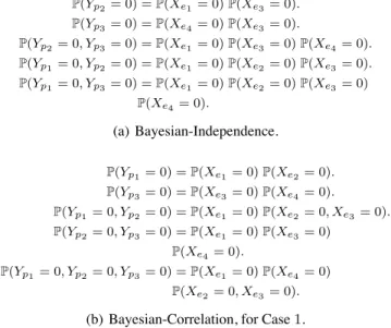
P(Yp1= 0) = P(Xe1= 0) P(Xe2= 0). P(Yp2= 0) = P(Xe1= 0) P(Xe3= 0). P(Yp3= 0) = P(Xe4= 0) P(Xe3= 0). P(Yp2= 0, Yp3= 0) = P(Xe1= 0) P(Xe3= 0) P(Xe4= 0). P(Yp1= 0, Yp2= 0) = P(Xe1= 0) P(Xe2= 0) P(Xe3= 0). P(Yp1= 0, Yp3= 0) = P(Xe1= 0) P(Xe2= 0) P(Xe3= 0) P(Xe4= 0). (a) Bayesian-Independence. P(Yp1= 0) = P(Xe1= 0) P(Xe2= 0). P(Yp3= 0) = P(Xe3= 0) P(Xe4= 0). P(Yp1= 0, Yp2= 0) = P(Xe1= 0) P(Xe2= 0, Xe3= 0). P(Yp2= 0, Yp3= 0) = P(Xe1= 0) P(Xe3= 0) P(Xe4= 0). P(Yp1= 0, Yp2= 0, Yp3= 0) = P(Xe1= 0) P(Xe4= 0) P(Xe2= 0, Xe3= 0).
(b) Bayesian-Correlation, for Case 1.
Figure 2: Equations formed by Boolean-Inference algo-rithms for the example of Fig. 1.
hence, the algorithm which assumes Homogeneity (Assump-tion 3), “favors” links that participate in more congested paths, i.e., the larger the number of congested paths in which a link participates, the more likely it is to be labeled as con-gested. For example, in the toy topology of Fig. 1, if the congested paths are {p1, p2, p3}, Sparsity will infer that the
congested links are {e1, e3} (because each of them
partici-pates in two congested paths).
Sparsity works best in scenarios where congestion is con-centrated in a few links; this is not the case, for instance, when there exists a lot of congestion at the edge of the net-work, i.e., many links adjacent to end-hosts are congested at the same time. For example, in Fig. 1, if links e2and e3
are both congested, that will cause the congested paths to be {p1, p2, p3}, and Sparsity will pick solution {e1, e3}, i.e.,
it will miss one congested link and falsely blame one good link.
Bayesian-Independence. This is a Bayesian Inference algorithm, i.e., of all the possible solutions, it picks the one that occurs with the highest probability. Hence, this algo-rithm consists of two steps: (i) Probability Computation, which monitors the network and learns the probability with which each solution occurs. (ii) Probabilistic Inference, which looks at the status of paths during each particular time inter-val and determines which set of links were most likely con-gested during that interval, based on the output of the previ-ous step; this is an NP-complete problem [11], so, this step uses an approximate algorithm. For example, in Fig. 1, if the congested paths are {p1, p2, p3}, Bayesian-Independence will
consider all 8 possible solutions and pick the one that occurs with the highest probability.
paths, learns the probability that each set of paths is con-gested and, from these, computes the probability that each link is congested; under the Independence assumption (As-sumption 4), it then computes the probability of each solu-tion. We illustrate with the example of Fig. 1: First, the method computes the probability that p1 is good, which is
equal to the probability that e1 and e2are both good since
it assumes links are independent. It forms the first equa-tion in Fig. 2(a). In the same way, it computes the prob-ability that each path and each pair of paths is good and forms the remaining equations in Fig. 2(a). The resulting system has four unknowns (one for each link) and four lin-early independent equations, hence, gives us the probabil-ity that each link is good. Assuming Independence, we can therefore easily compute the probability of each particular solution, e.g., the probability of solution Ec = {e
1, e3} is
P(Xe1= 1) P(Xe2= 0) P(Xe3= 1) P(Xe4 = 0).
Bayesian-Independence needs the Independence assump-tion, in order to form equations by combining probabili-ties related to different links. As previous work has already pointed out [9], this assumption does not always hold, which causes Bayesian-Independence to compute some probabili-ties incorrectly, leading to incorrect inference. For example, suppose that, in Fig. 1, links e1 and e4 are always good,
while e2and e3are perfectly correlated (either both are
con-gested or both are good). This means that P(Xe2 = 0, Xe3 =
0) != P(Xe2 = 0) P(Xe3 = 0), and the last two equations
in Fig. 2(a) are wrong. As a result, Bayesian-Independence incorrectly determines that {e1, e3} is the solution with the
highest probability and always picks it over the correct one, {e2, e3}.
A more subtle source of inaccuracy in the Probabilistic Inference step is the following: Bayesian-Independence de-termines whether link eiwas congested during a particular
time interval based on the probability that link ei is
con-gested during any time interval. More formally, Bayesian-Independence approximates the value of random variable Xei(t) with its expected value E[Xei(t)] = P(Xei = 1).
We illustrate with an example. Suppose that the Probability Computation module observes the network in Fig. 1 for an hour and computes, among others, the following probabili-ties:
P(Xe1 = 1, Xe2= 0, Xe3 = 0, Xe4 = 0) = 0.8.
P(Xe1 = 1, Xe2= 1, Xe3 = 0, Xe4 = 0) = 0.1.
This means that, during the one hour of monitoring, {e1}
was the only congested link in the network for 80% of the time, while {e1, e2} were the only congested links in the
network for 10% of the time. Now suppose that during the last 1-minute interval within this hour, the congested paths are {p1, p2}; the Probabilistic Inference module determines
that there are two possible solutions for this interval, {e1}
and {e1, e2}, and picks the first one (because it has a higher
probability associated with it). In essence, Probabilistic In-ference determines that this solution is more likely to have
occurred during the last minute, because it occurred more frequently over the last hour.
In practice, we cannot tell whether this approximation works, unless we have “insider information” on network conditions. For example, consider a link that is normally congested very rarely, and Probability Computation correctly computes a low congestion probability for it; suppose this link incurs a technical failure or comes under a flooding attack and be-comes severely congested for a few time intervals; unless we already know when this failure/attack occurs and how long it lasts, Probabilistic Inference will not pick this link as congested (because it has a low congestion probability associated with it). So, even if Probability Computation cor-rectly computes for what fraction of time a link is congested, Probabilistic Inference cannot use this information correctly, because it operates at a different time scale.
Finally, the Probabilistic Inference step uses an approxi-mate algorithm to pick the solution that occurred with the highest probability, which means that it does not always pick the right one.
To summarize, Bayesian-Independence introduces three additional sources of inaccuracy: the Independence assump-tion (used in both steps), the fact that it approximates the value of random variable Xei(t) with its expected value (in
the Probabilistic Inference step), and the use of an approx-imate algorithm to pick the solution that occurred with the highest probability (also in the Probabilistic Inference step). Bayesian-Correlation. In an effort to remove one source of inaccuracy, we developed a new inference algorithm that takes into account link correlations. It is similar to Bayesian-Independence (it also consists of a Probability Computation and a Probabilistic Inference step), however, in the former step, instead of Independence, it assumes Correlation Sets (Assumption 5). For instance, in the example of Fig. 1, Case 1, it treats P(Xe2 = 0, Xe3 = 0) as an extra
un-known, as opposed to mistakenly breaking it into P(Xe2 =
0) P(Xe3 = 0), and forms the equations in Fig. 2(b). The
resulting system has 5 unknowns (one for each link plus one for the pair of correlated links {e2, e3}) and 5 linearly
inde-pendent equations, hence, gives us the probability that each set of links is good. Once we know these probabilities, we can compute the probability of each solution [9].
However, taking link correlations into account comes at the price of introducing extra unknowns, and we can com-pute all of them if and only if the Identifiability++ condi-tion (Condicondi-tion 2) holds. For instance, in the example of Fig. 1, Case 2, it is impossible to compute the probability that {e1, e4} are both good or the probability that {e2, e3}
are both good. The intuition is the following: both these sets of links are traversed by the same set of paths, {p1, p2, p3};
this makes it impossible to distinguish one pair from the other based on path observations and to compute the prob-ability that each pair is good. So, the Probprob-ability Compu-tation step of Bayesian-Correlation cannot always compute the probability of all solutions, because the Identifiability++
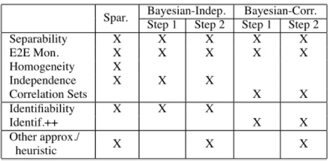
Spar. Bayesian-Indep. Bayesian-Corr. Step 1 Step 2 Step 1 Step 2 Separability X X X X X E2E Mon. X X X X X Homogeneity X Independence X X X Correlation Sets X X Identifiability X X X Identif.++ X X Other approx./ X X X heuristic
Table 2: Sources of inaccuracy for Boolean Inference algorithms: assumptions, conditions, and approxima-tions/heuristics.
condition does not always hold. As a result, the Probabilistic Inference step does not have all the information it needs to pick the likeliest solution; in the particular example consid-ered above, if the congested paths are {p1, p2, p3}, it picks
at random one of the solutions {e1, e4} or {e2, e3}.
To summarize, Bayesian-Correlation introduces four ad-ditional sources of inaccuracy: the Correlation Sets assump-tion and—like Bayesian-Independence—the fact that it ap-proximates the values of random variables with their ex-pected values and the use of an approximate algorithm to pick the solution that occurred with the highest probability (in the Probabilistic Inference step).
Conclusion. Each inference algorithm introduces its own sources of inaccuracy (summary in Table 2), and there is no basis for arguing that one algorithm covers more cases than the others.
3.2 Experiments
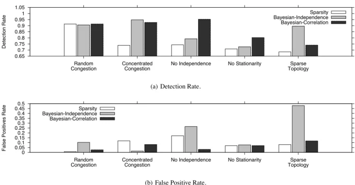
We now look at the performance of the three Inference al-gorithms under various scenarios (Fig. 3). We assume that Separability, E2E Monitoring, and Correlation Sets always hold, because this is the weakest set of assumptions under which we can solve Boolean Inference; the rest of the as-sumptions and conditions in Table 2 may or may not hold, depending on the scenario.
Metrics. We consider two metrics: during a particular time interval, the detection rate of an algorithm is the frac-tion of congested links that the algorithm correctly identified as congested; the false positive rate of an algorithm is the fraction of links incorrectly identified as congested out of all links inferred as congested by the algorithm. Each detection rate and false-positive rate we show is an average over 1000 time intervals.
Topologies. We use two kinds of topologies: the Sparse topologies are real topologies, given to us by the source ISP; the Brite topologies are synthetic topologies.
Each Sparse topology was obtained in the following way. The operator of the source ISP performed traceroutes from a few end-hosts located inside her network toward a large number of external end-hosts; she discarded all incomplete traceroutes. In this way, she collected a router-level graph
(where each vertex corresponds to an IP router and each edge corresponds to an IP-level link). Moreover, she mapped each IP router to an Autonomous System (AS) and created an AS-level graph, where each vertex corresponds to a border router and each edge corresponds to an inter-domain link between border routers of peering ASes, or an intra-domain path be-tween two border routers of the same AS. The source ISP wants to monitor its peers at the AS level (it is not inter-ested in each peer’s internals), hence, we use the AS-level graph as the network topology. The router-level graph tells us how the links in the AS-level graph are correlated—if a router-level link becomes congested, then all the AS-level links that share this router-level link become congested at the same time.
Each Brite topology also consists of a router-level and an AS-level graph, each derived using the corresponding mod-ule of the Brite topology generator [1].
We show results for a representative Sparse topology of about 2000 links and a representative Brite topology of about 1000 links, each of them with 1500 paths—the results for other topologies were similar. The Identifiability++ condi-tion holds only for the Brite topologies.
Simulator. In the beginning of each experiment, we de-termine the probability that each (AS-level) link is congested and the degree of correlation between congested links (de-pending on whether they share underlying router-level links). In the experiments that we present here, only 10% of the links are assigned a non-zero congestion probability, which is chosen at random between 0 and 1. Which particular 10% of the links have a non-zero probability of congestion differs, depending on the scenario we are simulating.
Each experiment consists of multiple time intervals. In the beginning of each interval, we flip a biased coin for each link, to determine whether the link will be good or con-gested, such that we respect the individual and joint prob-abilities of congestion determined in the beginning of the experiment; if we determine that a link will be good (resp. congested) in this interval, we randomly assign to it a packet-loss rate between 0 and 0.01 (resp. 0.01 and 1), according to the loss model in [12] (and similar to the loss models in [13, 11]). In each interval, packets are sent along each path; for each packet that arrives at a given link, we flip a biased coin to determine whether it will be dropped or not, such that we respect the packet-loss rate assigned to the link in the begin-ning of the interval.
Random Congestion (Brite). In this scenario, the 10% of the links that have a non-zero congestion probability are chosen at random. As we see in Fig. 3, all Inference algo-rithms perform equally well: on average, they identify 90% of the congested links and miss fewer than 2% of them (ex-cept from Bayesian-Independence that misses 10%).
The intuition is the following. The Brite topology models a full AS-level topology, hence, it is relatively “dense,” i.e., paths tend to criss-cross. This is good for Inference algo-rithms, because the denser the topology, the higher the rank
0.65 0.7 0.75 0.8 0.85 0.9 0.95 1 1.05 Random
Congestion ConcentratedCongestion No Independence No Stationarity TopologySparse
Detection Rate
Sparsity Bayesian-Independence Bayesian-Correlation
(a) Detection Rate.
0 0.05 0.1 0.15 0.2 0.25 0.3 0.35 0.4 0.45 0.5 Random
Congestion ConcentratedCongestion No Independence No Stationarity TopologySparse
False Positives Rate
Sparsity Bayesian-Independence Bayesian-Correlation
(b) False Positive Rate.
Figure 3: Performance of inference algorithms under various realistic congestion scenarios, when 10% of the network links have a positive probability of being congested.
of the resulting system of equations and the fewer the pos-sible solutions to each observation—which means that the heuristic/approximate aspect of each algorithm is exercised less. Bayesian-Independence performs slightly worse, be-cause it assumes that links are independent, whereas, in sev-eral time intervals, some of the congested links happen to be correlated (share an underlying router-level link).
Concentrated Congestion (Brite). In this scenario, the 10% of the links that have a non-zero probability of con-gestion are chosen to be located toward the edge of the net-work, i.e., there is no congestion at the core. As we see in Fig. 3, Sparsity’s detection rate drops to 75%, while its false-positive rate rises to 10%. This happens because Spar-sity assumes Homogeneity and picks links that are traversed by many congested paths, hence it is more likely to pick so-lutions that involve links located close to the core of the net-work. This result does not imply that Sparsity is worse than the other algorithms—just that it performs worse in this par-ticular scenario.
No Independence (Brite). In this scenario, the 10% of the links that have a non-zero probability of congestion are chosen such that each of them is correlated with at least one other. As we see in Fig. 3, Bayesian-Independence’s detec-tion rate drops below 80%, while its false-positive rate rises to 25%; this happens because its Probability Computation part assumes Independence, hence learns the probability of each set of links incorrectly.
No Stationarity (Brite). This scenario is similar to the previous one, plus the congestion probabilities of links (the
10% of them, that is) change every few time intervals. As we see in Fig. 3, it is the turn of Bayesian-Correlation’s detec-tion rate to drop below 80%; this happens because its Prob-abilistic Inference step assumes stationarity, i.e., it assumes that a solution is more likely to have occurred during the last time interval, just because it occurred more frequently throughout the entire experiment.
Sparse Topology. This scenario is similar to the first one (the 10% of the links that have a non-zero congestion prob-ability are chosen at random), but is applied to the Sparse as opposed to the Brite topology. As we see in Fig. 3, all Infer-ence algorithms suffer. The fact that Bayesian-IndependInfer-ence has a 90% detection rate should not be mistaken for success: it achieves this by aggressively marking links as congested, which results in a 45% false-positive rate.
The intuition is the following. The Sparse topology was created by running traceroutes from the source ISP to vari-ous Internet end-hosts. However, most traceroutes returned incomplete/inconclusive results and had to be discarded, which resulted in a “sparse” view, where few paths intersect one another. This is bad for Inference algorithms, because the sparser the topology, the lower the rank of the resulting sys-tem of equations—which means that each algorithm has to rely more on its heuristic/approximate aspect to pick a solu-tion. Note that we did not in any way engineer this scenario to make the Inference algorithms fail as we did in the previ-ous scenarios—we did not introduce extra link correlations or non-stationarity.
We should clarify that the Sparse topology is the most complete topology that the ISP operator was able to collect
with the resources (the monitoring points) she had at her dis-posal. One might argue that, if the operator had done a bet-ter job and collected a more complete (less sparse) topology, the Inference algorithms would have performed better. This is true, however, in our experience from working with the operator, piecing together a topology from traceroutes is a complex task—some routers respond to a traceroute probe through a different interface than the one where the probe was received, some routers do not respond to traceroute probes at all, while load-balancing interferes with traceroute results. Hence, we think it is fair to assume that operators are typi-cally not able to collect complete topologies.
Conclusion. Any Inference algorithm can perform badly under certain network conditions, and there is no evidence that such conditions do not occur in practice. Moreover, all Inference algorithms perform badly on Sparse topologies— in particular, each Inference algorithm performs worse on Sparse topologies under easy conditions (random conges-tion) than on Brite topologies under worst-case conditions (congestion at the edges for Sparsity, link correlations for Independence, and non-stationarity for Bayesian-Correlation).
4. SHIFTING GOALS
Until now, Probability Computation has been viewed as a step to enable Boolean Inference; we argue that, in the scenario considered in this work, Probability Computation is a useful problem to solve in its own right, and that it makes more sense to solve this problem than Boolean Inference.
If accurately solved, Boolean Inference would provide the source ISP with the status of each link in the network during each time interval. This information would enable the source ISP to attribute blame to a peer for a particular connectiv-ity/performance problem faced by the source ISP’s customers and/or request compensation in case an SLA has been vi-olated. However, as we saw in the last section, given the Sparse topology, state-of-the-art Inference algorithms yield a detection rate as low as 68% and a false-positive rate as high as 47%; attributing blame or extracting compensation is practically impossible based on this level of accuracy.
Probability Computation provides less information than Boolean Inference: if accurately solved, it would provide the source ISP with the congestion probability of each set of links in the network, i.e., how frequently each set of links are congested, but not which particular links were congested
when.
On the other hand, we have an algorithm (Step 1 of Bayesian-Correlation) that solves Probability Computation with fewer sources of inaccuracy than Boolean Inference algorithms:
!It assumes Separability, E2E Monitoring, and Correla-tion Sets—a weaker set of assumpCorrela-tions than those assumed by Sparsity and Bayesian-Independence.
! Unlike the Bayesian Inference algorithms (Bayesian-Independence and Bayesian-Correlation), our algorithm does not need to solve any NP complete problem.
!Unlike the Bayesian Inference algorithms, our algorithm does not need to approximate the value of any random vari-able with its expected value: if we compute that P(Xei =
1) = 0.8 over T time intervals, we interpret this as “ei
was congested for 80% of the T time intervals.” In contrast, the Bayesian Inference algorithms use the same information to infer during which particular intervals ei was congested.
When network conditions change over time, the Bayesian Inference algorithms may make the wrong decision (§3.1); our result, however, still holds, because it concerns the
av-erage behavior of the link over the T time intervals, and not
the diagnosis of the congested links over one time interval. The biggest challenge in solving Probability Computa-tion is complexity: there are as many unknowns as sets of links that belong to the same AS; in a real network, there may be billions of such sets, and it could take an imprac-tical amount of time to solve the corresponding system of equations. Hence, we design our algorithm to accurately compute a configurable subset of the computable probabili-ties, depending on the available resources. For instance, we can configure our algorithm to compute only the congestion probability of each individual link, or the congestion proba-bility of each set of one, two, or three links. This allows us to control the complexity of the algorithm and obtain useful information in a timely manner, even if we do not wait to solve Probability Computation completely (i.e., we do not learn the congestion probability of all sets of links).
In the next section, we support these claims with experi-mental results.
5. PROBABILITY COMPUTATION
In this section, we present an algorithm that solves the Probability Computation problem, assuming Separability, E2E Monitoring, and Correlation Sets (Assumptions 1, 2, and 5). In particular, our algorithm computes the congestion prob-ability of each correlation subset for which the following is true: there exists no other correlation subset in the network that is traversed by the same paths. When the Identifiabil-ity++ condition holds, this is true for all correlation subsets, which means that our algorithm computes the congestion probability of each set of links in the network.
After introducing a basic building block of the algorithm (§5.1) and our terminology and notation (§5.2), we describe the algorithm itself (§5.3), and evaluate it experimentally (§5.4).
5.1
A Basic Building Block
Informally, our algorithm forms a system with enough lin-early independent equations to compute as many congestion probabilities as possible. Each equation corresponds to a different set of paths, in the following way: consider a set of paths P ; by the Separability assumption, if all paths in P are good, then all links traversed by the paths in P (denoted by
Links(P )) are good; hence, we can write: P $ p∈P Yp= 0 = P $ e∈Links(P ) Xe= 0 = ' C∈C∗ P $ e∈Links(P )∩C Xe= 0 . (1)
In Fig. 1, Case 1, if we apply Eq. 1 to path set {p1}, we
obtain:
P(Yp1 = 0) = P(Xe1 = 0, Xe2 = 0)
= P(Xe1 = 0) P(Xe2 = 0). (2)
If we apply Eq. 1 to path set {p1, p2}, we obtain:
P(Yp1 = 0,Yp2 = 0) = P(Xe1 = 0, Xe2 = 0, Xe3= 0)
= P(Xe1= 0) P(Xe2 = 0, Xe3 = 0). (3)
We could form as many such equations as there are sets of paths in the network. A na¨ıve approach would be to con-sider all 2|P∗|
possible sets of paths in the network, form a system of that many equations, reduce this to a system of linearly independent equations3, and solve the latter. How-ever, processing 2|P∗|
equations is practically infeasible for any topology with more than a few tens of paths (our Sparse topology has roughly 1500 paths). We address this challenge by using a novel technique that forms the minimum number of equations needed, without considering all possible sets of paths.
5.2 Definitions and Notation
! The path coverage function Paths (E) maps a set of links E to the set of paths that traverse at least one of these links. In Fig. 1, Paths ({e1, e2}) = {p1, p2}, Paths ({e1, e3})
= {p1, p2, p3}.
! The link coverage function Links (P ) maps a set of paths P to the set of links traversed by at least one of these paths. In Fig. 1, Links ({p1}) = {e1, e2}, Links ({p1, p2}) =
{e1, e2, e3}.
!A correlation subset E is a non-empty subset of a corlation set, i.e., E ⊆ C for some correcorlation set C. We often re-fer to “all the possible correlation subsets” in the network; in Fig. 1, Case 1, these are {e1}, {e2}, {e3}, {e4}, {e2, e3}; in
Case 2, they are {e1}, {e2}, {e3}, {e4}, {e2, e3}, {e1, e4}.
!We define the complement of a correlation subset E that belongs to a correlation set C as ¯E = C \ E. In Fig. 1, Case 1, {e1} = ∅, {e2} = {e3}, and {e3} = {e2}, {e4} =
{e2, e3} = ∅.
!A correlation subset E is potentially congested if none of its links is traversed by a path that is always good, i.e., every path that traverses a link in E is congested during at 3If we consider the logarithm of Eq. 1, we obtain a linear equation.
least one time interval. In Fig. 1, Case 1, suppose path p3
is always good, whereas the other two paths are not; this means that links e3 and e4are always good, hence, the
po-tentially congested correlation subsets are {e1} and {e2}.
The congestion probability of any correlation subset that is not potentially congested is 0.
!If P is a set of paths and ˆE is an ordering of all the po-tentially congested correlation subsets, we define the vector Row(P, ˆE) as follows: we apply Eq. 1 to the set of paths P and we form a vector r, where
ri=
1, if the i-th correlation subset in ˆE appears in the equation for path set P
0, otherwise. Row(P, ˆE) is equal to r.
!If ˆP is an ordering of a set of path sets and ˆE is an or-dering of all the potentially congested correlation subsets, we define the matrix Matrix ( ˆP , ˆE) as follows: the i-th row of the matrix is equal to Row (Pi, ˆE), where Pi is the i-th
path set in ˆP. For example, in Fig. 1, Case 1, suppose all correlation subsets are potentially congested; given an or-dering of these correlation subsets ˆE = ${e1}, {e2}, {e3},
{e4}, {e2, e3}% and an ordering of path sets ˆP = ${p1}, {p1, p2}%,
Matrix( ˆP , ˆE) = + 1 1 0 0 0 1 0 0 0 1 , .
This matrix corresponds to the system of equations 2 and 3.
5.3
The Algorithm
To compute the congestion probability of each set of links, it is sufficient to compute the congestion probability of each potentially congested correlation subset—or, equivalently, for each potentially congested correlation subset E, compute the probability that all links in that subset are good [9], i.e.,
P -$ e∈E Xe= 0 . .
For instance, in Fig. 1, Case 1, if all the correlation subsets are potentially congested, it is sufficient to compute P(Xe1 =
0), P(Xe2 = 0), P(Xe3 = 0), P(Xe4 = 0), and P(Xe2 =
0, Xe3 = 0).
To compute these probabilities, our algorithm (Alg. 1) forms as many linearly independent equations as it can by applying Eq. 1 to different path sets. The input to the algo-rithm is an ordering ˆE of all the potentially congested corre-lation subsets that can appear in such equations.4The output
is an ordering of path sets ˆPto which we apply Eq. 1 to form a system of equations.
First, we form an initial list of path sets ˆP (lines 1 to 5). We ensure that each correlation subset E ∈ ˆE is tra-versed by at least one of the path sets in ˆP, namely path 4When Identifiability++ does not hold, there may exist correlation subsets that cannot appear in any equation. We give an example in our technical report [10].
Algorithm 1 Selection of Path Sets
Input: E:ˆ a list of potentially congested correlation subsets
Variables: Pˆ: a list of path sets P: a path set E: a correlation subset
1: Pˆ← "#
2: for all E ∈ ˆE do
3: P← Paths (E) \ Paths!¯ E" 4: Pˆ← ˆP+ P 5: end for 6: R ← Matrix ( ˆP , ˆE) 7: N ← NullSpace (R) 8: repeat 9: r ← 0
10: for all E ∈ SortByHammingWeight( ˆE, N) do
11: for all P ⊆ Paths (E) \ Paths!¯ E" do 12: r ← Row (P, ˆE) 13: if ||r × N|| > 0 then 14: Pˆ← ˆP+ P 15: go to line 21 16: else 17: r ← 0 18: end if 19: end for 20: end for 21: N ← NullSpaceUpdate (N, r)
22: until N has no columns left or r = 0
23: return ˆP Notation:
A \ B: subtract set B from set A ˆ
P+ P : add path set P to list of path sets ˆP
set Paths (E) \ Paths/¯
E0 (lines 2 and 3). We illustrate with an example. Suppose that, in Fig. 1, Case 1, all cor-relation subsets are potentially congested and we pick order-ing ˆE = ${e1}, {e2}, {e3}, {e4}, {e2, e3}%. After line 5 has
been executed, ˆPconsists of the path sets in the last column of the following table:
E E¯ Paths(E) Paths!¯ E" Paths(E) \ Paths!¯ E" {e1} ∅ {p1, p2} ∅ {p1, p2} {e2} {e3} {p1} {p2, p3} {p1} {e3} {e2} {p2, p3} {p1} {p2, p3} {e4} ∅ {p3} ∅ {p3} {e2, e3} ∅ {p1, p2, p3} ∅ {p1, p2, p3} If we apply Eq. 1 to each of the path sets in ˆP, we obtain the system of equations shown in Fig. 2(b). In this particu-lar example, the corresponding matrix Matrix ( ˆP , ˆE) has full column rank, which means that we can solve our system and compute, for each correlation subset, the probability that all links in that subset are good, hence also the congestion prob-ability of each set of links in the network. In general, how-ever, the resulting system of equations is under-determined, and we continue with the second part of the algorithm.
We augment the initial list of path sets ˆP by iteratively
Algorithm 2 N ullSpaceU pdate
Input: N: a matrix of size n × p r: a row vector of n elements
1: return#In− N∗1×r r×N∗1 $ N∗2:p Notation:
In: the identity matrix of size n
N∗1: the 1-st column of matrix N
N∗2:p: the matrix formed by taking columns
2 to p of N
adding path sets, such that we increase the rank of the associ-ated matrix Matrix ( ˆP , ˆE) (lines 6 to 22). More specifically, we first compute the matrix R associated with the initial list of path sets ˆP(line 6), as well as a matrix N, whose columns span the null space of R (line 7); the latter can be done us-ing standard techniques, like sus-ingular value decomposition or QR factorization. Next, we iteratively identify a path set P such that adding r = Row (P, ˆE) to the system matrix, increases the latter’s rank, and we add P to ˆP (lines 12 to 15). Every time we add a new path set to ˆP, we update the matrix N, such that its columns always span the null space of Matrix ( ˆP , ˆE) (line 21). We stop the iteration when N is left with 0 columns or there are no more path sets left to consider, i.e., the loop in line 10 finishes (line 22).
The first point worth noting is that identifying a new set of paths P such that Row (P, ˆE) increases the rank of the sys-tem matrix is not straightforward. If such a set of paths ex-ists, our algorithm finds it, because it iterates over all sets of paths (lines 10 and 11) and tests whether each of them satis-fies the corresponding condition (lines 12 and 13). However, to save time, the algorithm orders the sets of paths such that it first tries those that are more likely to satisfy the condition (this is the role of the SortByHammingWeight function). Intuitively, if the i-th element of vector r is non-zero and the i-th row of matrix N has many non-zero elements, then ||r × N|| > 0 is likely to be true. Thus, our algorithm picks the row of N with the largest number of non-zero elements (the largest Hamming weight); suppose that this row corre-sponds to a correlation subset E (line 10). Then, it looks for any path set P that traverses E (line 11), and picks the first one that satisfies the condition (lines 12 to 15). The SortByHammingWeight helps us pick the correlation sub-set E—it outputs an ordering of the correlation subsub-sets in ˆE such that the first element in that ordering corresponds to the row of matrix N with the largest Hamming weight.
The second point worth noting about the algorithm is that computing the null space of a matrix with thousands of rows takes a significant amount of time, and doing this at every iteration would render the algorithm practically useless. In-stead, the N ullSpaceU pdate function (Alg. 2) updates the null space incrementally, i.e., given the null space computed in the previous iteration, it efficiently updates the null space. Complexity. The complexity of our algorithm is O(n31+
n2
0 0.05 0.1 0.15 0.2 Random
CongestionConcentratedCongestion No Independence
Mean of the Absolute Error
Independence Correlation-heuristic Correlation-complete
(a) The mean of the absolute error under various congestion sce-narios, when computing the congestion probability of individual links. Brite topologies.
0 0.05 0.1 0.15 0.2 0.25 0.3 Random
CongestionConcentratedCongestion No Independence
Mean of the Absolute Error
Independence Correlation-heuristic Correlation-complete
(b) The mean of the absolute error under various congestion sce-narios, when computing the congestion probability of individual links. Sparse topologies.
0 0.2 0.4 0.6 0.8 1 0 0.2 0.4 0.6 0.8 1 CDF Absolute Error Independence Correlation-heuristic Correlation-complete
(c) CDF of the absolute error for the “No Independence” con-gestion scenario, when computing the concon-gestion probability of individual links. Sparse topologies.
0 0.05 0.1 0.15 0.2 Brite Sparse
Mean of the Absolute Error
links correlation subsets
(d) The mean of the absolute error of the Correlation-complete al-gorithm in the “No Independence” scenario, when computing the congestion probability of individual links and correlation subsets.
Figure 4: Performance of Probability Computation algorithms for Brite and Sparse topologies. congested correlation subsets, n2= maxE∈ ˆE|Paths (E) | is
the maximum number of paths that traverse the same poten-tially congested correlation subset, n3 is the nullity of the
initial system matrix Matrix ( ˆP , ˆE). We express complexity as a function of these three parameters, because any one of them can dominate the other two, depending on the topology and the congestion scenario. The proof can be found in our technical report [10].
5.4 Experiments
We now look at the performance of our algorithm (we la-bel it Correlation-complete) and compare it to the two most related pieces of work: (i) Independence [11], which is the Probability Computation step of the Bayesian-Independence algorithm; (ii)Correlation-heuristic [9], an earlier heuristic that, under the Correlation Sets assumption, computes the probability that each individual link is congested.
We reconsider all congestion scenarios described in Sec-tion 3.2: Brite (Fig. 4(a)) and Sparse (Fig. 4(b)) topologies, where 10% of the links have a non-zero probability of being congested. The links with a non-zero congestion probabil-ity are chosen either at random (Random Congestion), or chosen to be located toward the edge of the network (Con-centrated Congestion), or chosen such that each of them is correlated with at least one other link (No Independence). In addition, in each of these scenarios, the congestion
prob-ability of each link changes every few time intervals, i.e., we add the “No Stationarity” scenario on top of each of the above scenarios described in Section 3.2.
First, we evaluate how accurately each algorithm com-putes the congestion probability of each individual link. For each link, we determine the absolute error between the ac-tual congestion probability (the one assigned by the simu-lator) and the one inferred by each algorithm; we show the mean of the absolute error for all potentially congested links, i.e., all links which are not traversed by any good path.
For the Brite topologies (Fig. 4(a)), in the “Random Con-gestion” and “Concentrated ConCon-gestion” scenarios, all algo-rithms perform well, with a mean absolute error below 0.07; for the “No Independence” scenario, the error of the Inde-pendence algorithm doubles compared to that of the alterna-tives (because it ignores link correlations).
For the Sparse topologies (Fig. 4(b)), the performance of the Correlation-heuristic and Independence algorithms de-grades, because these algorithms create a significantly larger number of equations than ours, which introduces more noise when solving the system. For the “No Independence” sce-nario, the mean of the absolute error of the Independence al-gorithm is 3 times larger than that achieved by our alal-gorithm. Since this scenario is the most challenging for all algorithms, we also show the cumulative distribution function (CDF) of the absolute error for each algorithm (Fig. 4(c)). For a
per-fect algorithm, this CDF would be a single point at x = 0, y = 100%, i.e., the algorithm would compute each con-gestion probability with an absolute error of 0. In general, the earlier the CDF hits the y = 100% line, the better the performance of the corresponding algorithm. Correlation-heuristic is able to compute accurately (with an absolute er-ror below 0.1) the congestion probability of only 65% of the links, while the Independence algorithm is more uniformly inaccurate for 50% of the links. Our algorithm does better, with an absolute error less than 0.1 for 80% of the links.
We also show how accurately our algorithm computes the congestion probabilities of different sets of links, not just individual links (Fig. 4(d)). Knowing these probabilities re-veals which links within each peer are actually correlated; this can be useful for computing “disjoint” paths to some destination, i.e., paths that are not likely to fail at the same time. Our algorithm performs well: even in the “No Inde-pendence” scenario, it accurately computes the congestion probability of all correlation subsets for Brite topologies, or a significant number (depending on available resources) of correlation subsets for Sparse topologies, with a mean abso-lute error of 0.1 or less.
Conclusion. The Probability Computation problem can be solved accurately, even on sparse topologies with link correlations and non-stationary network conditions.
6. RELATED WORK
Network performance tomography, which infers link char-acteristics from end-to-end path measurements, is an ill-posed inverse problem that has been well studied in the last decade.
The initial methods relied on temporal correlation to infer the loss rate of network links, either by sending multicast probe packets (which are perfectly correlated on multicast links) [4, 3, 2], or by sending unicast probe packets back to back (which are strongly correlated on shared links), as an emulation of multicast packets [5, 7]. Multicast is not widely deployed, and groups of unicast packets require substantial development and administrative costs, hence it is not easy to rely on temporal correlations.
The set of methods [12, 8, 11] that followed use only unicast end-to-end flows for the simpler goal of identifying the congested links (i.e., identifying if the link loss rate or delay exceeds some threshold, instead of computing their actual value). As different assignments are possible, these “Boolean” network-tomographic methods use additional in-formation or assumptions. In Sections 2 and 3, we discussed these assumptions and their practical impact in detail.
We show that, in the scenario of an ISP that wants to mon-itor the performance of its peers, it is more useful to compute the probabilities that links are congested rather than identify the congested links. We propose an algorithm that computes these probabilities without assuming link independence (as opposed to the method in [11]) and achieves significantly higher accuracy for sparse topologies than the heuristic pro-posed in [9].
7.
CONCLUSION
We considered a real scenario where network performance tomography could be useful: a Tier-1 ISP wants to monitor the congestion status of its peers. In principle, this could be achieved using Boolean Inference; in practice, in turned out that, in this scenario, Boolean Inference cannot be solved accurately enough to be useful. We argued that it makes more sense to solve the Congestion Probability Computa-tion problem—compute how frequently each peer’s links are congested as opposed to infer which particular links are con-gested when. We presented an algorithm that solves this problem accurately under weaker assumptions than those required by Boolean Inference and more challenging net-work conditions (sparse topologies, link correlations, and non-stationary network dynamics).
Acknowledgments
This work was supported by grant ManCom 2110 of the Hasler Foundation, Bern, Switzerland, and by an Ambizone grant from the Swiss National Science Foundation. We would like to thank our shepherd Rocky K.C. Chang and the anony-mous reviewers for their constructive feedback.
8.
REFERENCES
[1] Boston University Representative Internet Topology Generator. http://www.cs.bu.edu/brite/.
[2] A. Adams, T. Bu, T. Friedman, J. Horowitz, D. Towstey, R. Caceres, N. Duffield, F. L. Presti, S. B. Moon, and V. Paxson. The Use of End-to-end Multicast Measurements for Characterizing Internal Network Behavior. IEEE Communications Magazine, May 2000. [3] T. Bu, N. Duffield, F. L. Presti, and D. Towsley. Network
Tomography on General Topologies. In Proceedings of the ACM
SIGMETRICS Conference, 2002.
[4] R. Caceres, N. G. Duffield, J. Horowitz, and D. Towsley.
Multicast-based Inference of Network-Internal Loss Characteristics.
IEEE Transactions on Information Theory, 45:2462–2480, 1999.
[5] M. Coates and R. Nowak. Network Loss Inference Using Unicast End-to-End Measurement. In Proceedings of the ITC Specialist
Seminar on IP Traffic Measurement, Modeling and Management,
2000.
[6] A. Dhamdhere, R. Teixeira, C. Drovolis, and C. Diot. Netdiagnoser: Troubleshooting network unreachabilities usind end-to-end probes and routing data. In Proceedings of ACM Conext, 2007.
[7] N. Duffield, F. L. Presti, V. Paxson, and D. Towsley. Inferring Link Loss Using Striped Unicast Probes. In Proceedings of the IEEE
INFOCOM Conference, 2001.
[8] N. G. Duffield. Network Tomography of Binary Network Performance Characteristics. IEEE Transactions on Information
Theory, 52(12):5373–5388, December 2006.
[9] D. Ghita, K. Argyraki, and P. Thiran. Network Tomography on Correlated Links. In Proceedings of the ACM IMC Conference, 2010. [10] D. Ghita, K. Argyraki, and P. Thiran. Rethinking boolean network
tomography. Technical report, EPFL, 2011.
[11] H. X. Nguyen and P. Thiran. The Boolean Solution to the Congested IP Link Location Problem: Theory and Practice. In Proceedings of
the IEEE INFOCOM Conference, 2007.
[12] V. N. Padmanabhan, L. Qiu, and H. J. Wang. Server-based Inference of Internet Performance. In Proceedings of the IEEE INFOCOM
Conference, 2003.
[13] H. H. Song, L. Qiu, and Y. Zhang. NetQuest: A Flexible Framework for Large-Scale Network Measurement. In Proceedings of the ACM