Cybernetics and Systems Analysis, Vol. 37, No. 6, 2001
SOME MARKOVIAN QUEUING RETRIAL SYSTEMS UNDER LIGHT-TRAFFIC CONDITIONS
V. V. Anisimova and M. Kurtulushb UDC 519.21
The asymptotic behavior of the time of the first loss of a demand in Markovian single-channel and multichannel queuing retrial systems with a finite buffer and an external Markovian environment is analyzed. Two cases are studied: (a) the ratio of the input rate to the service rate tends to zero and (b) the ratio of the input rate to the service rate and the ratio of the input rate to the retrial rate tend to zero simultaneously. The method of so-called S-sets and the concept of a monotone structure introduced by Anisimov are used to prove the exponential approximation of the time of the first call loss and Poisson approximation of a flow of lost demands for both cases.
Keywords: Markovian queuing systems, retrials, light-traffic conditions, S-sets, Markovian
environment.
INTRODUCTION
Mathematical models of actual computer systems and communication networks have, as a rule, a complex hierarchical structure and operate at different time scales. For example, real time and processor time run at different rates. Analytical solution for such models can be found only in special cases; therefore, asymptotic and approximating methods are important for analysis and simulation of such systems. Many practically important models have a so-called small parameter, such as the order of failure probabilities or rates or the ratioρ of the mean service time to the mean time between arrivals of demands. In queuing theory, a system withρ→0 is usually called a light traffic system. In reliability theory, a system with a small ratio of the mean recovery time to the mean time between failures is called an element-reliable system or a fast-recovery system. The use of small parameters intensified the analysis of “rare” events in reliability and queuing theories [1, 2]. Note that the term “quick service” was used in [3, 4] to analyze queuing systems with asymptotically small service time. In applications, rare events usually mean various failures, loss of demands, leaving some domain, excess of a level, etc.
An asymptotic analysis is made of the demand loss time in Markovian service retrial systems under light-traffic conditions. Queuing retrial systems are characterized by the following property: a demand arriving at a system with all servicing servers and buffers occupied is put on a special retrial queue and the service demand is repeated after some random time. Such a property is inherent in many models of computer and telecommunication networks. Let us call a retrial queue an orbit. Systems with retrial queues were studied in [5–8] in detail. Note that explicit formulas for stationary and reliability characteristics cannot be obtained even for Markovian models of single-channel systems. The dimension of the problem increases exponentially with the number of channels. Thus, it is of interest to derive simple approximate formulas oriented to various applications.
In studying various classes of computer and telecommunication networks, various processes in the system often develop at different time scales. This means that transition probabilities or intensities have different orders of smallness. To analyze such classes of models, a special concept of a so-called S-set (an asymptotically connected set) was introduced in [9, 10]. The method of S-sets allows us to study the asymptotical behavior of the time of the first loss of a demand for wide classes of Markovian and semi-Markovian queuing models with a finite set of states and under quick-recovery or light-traffic conditions. Various applications of this method are presented in [11–17].
1060-0396/01/3706-0876$25.00 ©2001 Plenum Publishing Corporation a
Taras Shevchenko University, Kiev, Ukraine. Bilkent University, Ankara, Turkey. bBilkent University, Ankara, Turkey. Translated from Kibernetika i Sistemnyi Analiz, No. 6, pp. 110-126, November-December, 2001. Original article submitted October 26, 2000.
Another area in the asymptotic analysis of queuing systems is the diffusion approximation. The asymptotic technique of switching processes was used in [15, 18] to obtain some results for some classes of queuing systems. The diffusion approximation of some classes of retrial queuing systems was studied in [19–22]. An asymptotic analysis of the first-loss time in retrial systems was mainly made for classical single-channel Markovian models [23].
The asymptotical behavior of the first-loss time and a lost-demand flow in Markovian multichannel retrial systems is studied here. We assume that the characteristics of the system depend on some normalizing parameter n, n→ ∞. It is expedient to use the following terminology. Let the case where the ratio of the input-flow parameter to the service rate tends to zero be called an intensive service. The case where the ratio of the input-flow parameter to the retrial intensity tends to zero is called intensive retrial.
The present paper is organized as follows. In Section 2, the asymptotical behavior of the first-loss time is studied for single-channel Markovian retrial queuing systems under conditions of intensive service and ordinary or intensive retrials. Cases are also considered where the parameters depend on the queue size and the state of the Markovian environment. Multichannel systems are considered in Section 3. The results of the asymptotic analysis of the time of the first exit from the
S-set and structures of the state space are illustrated in the Appendix.
2. SINGLE-CHANNEL RETRIAL SYSTEMS
Let us consider a single-channel retrial system with m waiting places in the orbit (for retrials) and losses. The system input flow is Poisson with a parameter λ. The input demands are identified as primary. If the server (channel) is free, the arriving demand is immediately serviced and leaves the system once the service is completed. If the server is busy, the demand is put on the retrial queue (in an orbit) if the queue consists of less than m demands. Otherwise, the demand is considered lost. Each demand in the orbit generates, independently of the other demands, a Poisson flow of calls to the server (secondary demands) with intensityν. If a secondary demand discovers that the server is free, then it is immediately serviced and leaves the system once the service is completed. For the sake of simplicity, we assume that the service time has the same exponential distribution with the parameter µ for the initial and secondary demands. Let such a model be called
M /M /1/m wr/ .
Using the results presented in the Appendix (on the asymptotic exponentiality of the time of the first exit from the subset of states forming a monotone structure), let us study the asymptotic behavior of the first-loss time for systems with intensive service, with intensive service and intensive retrial, and for systems in a Markovian random environment. Assume that the intensities µ µ= n and ν ν= n can depend on some normalizing parameter n, n→ ∞. Without loss of generality, assume also that the intensity of the input flow λ does not depend on n. Let us consider the following cases.
Case 1. Let µn =nµ (intensive service), νn =ν (ordinary retrial), and n→ ∞.
Case 2. Let µn =nµ (intensive service), νn =Vnν (intensive retrial), n→ ∞, and Vn → ∞.
LetΩn( , ) be the time of the first loss of a demand provided that Qj q n( )0 =qandδn( )0 =j, 0≤ ≤q m, j=0 1, , and
Yn( ) be the number of lost demands on the interval [ , ]t 0 t . Denote by Qn( ), tt ≥0, the number of demands in the orbit at the time t, and let the component δn( ) be the state of the server at the time t (t δn( )t =1 if the server is busy and δn( )t =0 otherwise).
2.1. Case 1: Intensive Service
THEOREM 2.1. For the model described above under intensive service, if λ>0, µ>0, and ν>0, then the distribution of n− −m 1Ωn( , ), irrespective of the initial state ( , )j q j q , 0≤ ≤q m, j=0 1, , weakly converges to the exponential distribution lim ( , ) exp n m n n j q t t → ∞ − − ≥ = − P { 1Ω } { Λ}, t>0, where Λ = + + = =
∏
λ ρ ν λ ν ρ λ µ m m k m m k 1 1 ! ( ), / . (2.1)Proof. Let us consider a multidimensional process zn( )t =(δn( ),t Qn( ))t , t≥0. It is a homogeneous Markovian process (MP) with continuous time and a set of states Z={( , ),j q j=0 1, ;q=0 1, , . . . ,m}. The process zn( ) describes thet
of waiting places in the orbit and putz$ ( ) ( ( ), $ ( ))n t = δn t Qn t . Note thatz$ ( )n t is an MP in {0 1, } {× 0 1, , . . .}. ThenΩn( , ) isj q
equivalent to the time of the first exit of z$ ( )n t from the subset Z:
Ωn( , )j q =min{t t: >0, $ ( )Qn t >m provided that $ ( )Qn 0 =q, δn( )0 = j}.
One can easily calculate the intensities of transitions for zn( ) and see that Z forms a monotone structure (seet
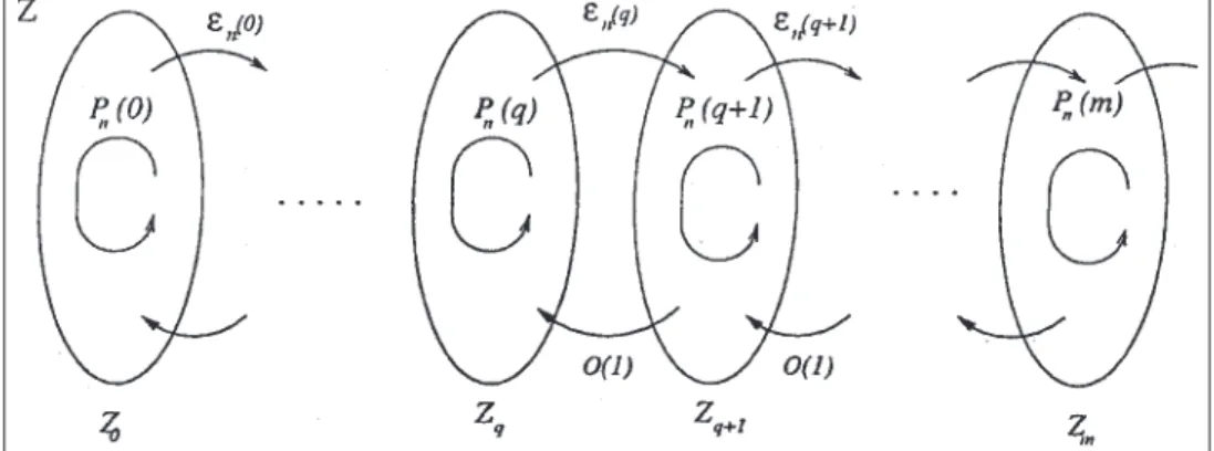
Definition A2). Here, the set Zq ={( , ),j q j=0 1 forms a q-level for each q, } =0 1, , . . . ,m (see Fig. 1).
A monotone structure for the model is presented in Fig. 2, where αq =qν λ( +qν)−1, βq =λ λ( +qν)−1, and
εn( )q =λ/ (nµ).
In the state ( , )j q , the process z$ ( )n t spends exponential time with the parameter Λn( , )j q = +λ nµ if j=1 and
Λn( , )j q = +λ qν if j=0. Transition probabilities are calculated by the formulas
pn(( , ), ( ,1 q 1q+1))∼n−1ρ→0, pn(( , ), ( ,0 q 1 q−1))=qν λ( +qν)−1, pn(( , ), ( , ))0 q 1 q =λ λ( +qν)−1, pn(( , ), ( , ))1 q 0 q =nµ λ( +nµ)−1→1.
Denote by πn( )q =(πn( , ),0 q πn( , ))1 q the stationary distribution of the embedded Markov chain for zn( ). Lett
πi =π( , )i 0 , i=0 1, , (π=(π π0, 1)) be a stationary distribution of states at the level Z0 ={( , ), ( , ) (0-level) in the limit.0 0 1 0} Since Z0 forms one significant class, the limit exists and it is easy to calculate that π0 =π1=1 2/ .
Further, the matrices A j( ) and P j( ) in the matrix relations of Theorem A2 have the form
A j( ) / = 0 0 0 λ µ , P j( )= + j 0 1 0 λ λ ν .
Fig. 1. Monotone structure.
Fig. 2. Monotone structure for a single-channel quick-service system. Level (q−1) Level (q) Level (q+1)
Therefore, the stationary distribution for the embedded Markov chain of the process zn( ) has the formt π π λ µ λ λ ν n j q q I j ( ) / ( ) = − + + = −
∏
0 1 0 0 0 0 1 1 0 + ≥ −1 1 1 1 1 n ( ο( )), q . Transformations yield π π ρ ν λ ν ο n q q q j q q n q j e q ( ) ! ( ) ( ( )), , , . . . = + + = =∏
1 1 1 1 2 1 1 ,where ρ λ µ= / and e is a unit vector. Note that πn ε s q n q O s ( )= ( ) = −
∏
0 1 . Similarly, we obtain g Z n m j n G n m m m j m m ( ) ! ( )( ( )) ( = + + + + = + = +∏
1 1 1 1 1 1 1 1 1 1 π ρ ν λ ν ο ο( ))1 .If in (A3) we put βn =n− −m 1, then a( , )j q ( )θ =G −1λ θ−1 for q=0, j=0 and a( , )j q ( )θ =0 otherwise. Thus, for A ( )θ in (A4) we have A( )θ =π0(Gλ)−1θ.
Finally, performing transformations we obtain that the parameter of the limit exponential distribution has the form
Λ =π0(Gλ)−1, which corresponds to (2.1).
2.1.1. Dependence of the Parameters on the System State. This result may be extended to the case where the intensities depend on the queue size. Let λ( )k , µ( )k , k=0,m, and ν( )k , k=1,m, be given. Then when Q tn( )=k, the instantaneous intensity of the input flow is λ( )k , the service intensity is nµ ( ), kk =0,m, and the retrial intensity is ν( )k , k=1,m. Using the same technique, we obtain the following statement.
Statement 2.1. Let
∏
mk=0( ( )λ k µ( ))k∏
mj=1 νj >0. Then, under the above assumptions, the distributionn− −m 1Ωn( , ) weakly converges to an exponential distribution with the parameterj q
Λ = + + + + = = −
∏
∏
λ λ µ λ ν ν ( ) ! ( ) ( ) ( ) ( ) ( ) ( 0 1 1 1 1 0 0 1 m k k k k k k k m k m ) .Remark 2.1. In both cases (homogeneity or dependence on the state), the process Y n( m+1t)on any interval [ ,0 T] weakly converges (in the sense of weak convergence of finite-dimensional distributions and measures in the Skorokhod space DT) to the ordinary Poisson process with the same parameter Λ.
2.2. Intensive Service and Intensive Retrial
THEOREM 2.2. Under conditions of intensive service and intensive retrial forλ>0,µ>0, andν>0, the distribution
n− −m 1Ωn( , ), irrespective of the initial state, weakly converges to an exponential distribution with the parameterj q Λ, where
Λ =λρm+1 .
Proof. It is similar to that of Theorem 2.1. Let us consider an auxiliary MPz$ ( ) ( ( ), $ ( ))n t = δn t Qn t , t≥0. It is easy to verify that the set Z forms a monotone structure and the subset Zq ={( , ),j q j=0 is a q-level, q} =0 1, , . . . ,m. The process $ ( )
zn t is in the state ( , )j q during an exponential time with the parameterΛn( , )j q = +λ nµ if j=1 andΛn( , )j q = +λ qVnν if j=0. Put ρ λ µ= / . The transition probabilities for the embedded MP have the form
pn(( , ), ( ,1q 1 q+1))∼n−1ρ→0, pn(( , ), ( ,0 q 1 q−1))=qVnν λ( +qVnν)−1→1,
Denote by πn( )q =(πn( , ),0 q πn( , ))1 q , q≥0, the stationary distribution for z$ ( )n t and let πj =π0( , ),j 0
j=0 1, , (π=(π π0, 1))be a stationary distribution for the level Z0 in the limit. It is easy to see thatπ0 =π1 =1 2/ . Further, in the relations of Theorem A2, the matrices A j( ) and P j( +1 have the form)
A j( )= 0 0 0 ρ , P j( + =) 1 0 1 0 0 . Performing transformations, we have
πn q π q ρq ο n e ( )= 1 1 (1+ ( ))1 , g Z n n( )= m+ m+ ( + ( )) 1 1 1 1 1 1 π ρ ο .
Substitutingβn =n− −m 1, we finally obtainΛ =λρm+1. Note that it is only this case where the result does not depend on the values of ν>0. However if ν=0 or ν ν= n →0, then the result will be different.
Let us now consider the case of dependence on the state. Let for Q tn( )=qthe intensity of the input flow beλ( )q , the
service intensity be nµ ( ), qq =0,m, and the retrial intensity be Vnν( ), qq =1,m. Here n→ ∞ and Vn → ∞. Remark 2.2. If
∏
mk=0( ( )λ k µ( ))k∏
mj=1ν( )j >0, then the statement of Theorem 2.2 is true, whereΛ = =
∏
λ λ µ ( ) ( ) ( ) 0 0 k m k k .Here, the process Y n( m+1t) weakly converges to the ordinary Poisson process with the parameter Λ. In this case, the result also does not depend on the values of ν( )j>0, j=1,m.
2.3. Dependence on the System State and Markovian Environment
Let us consider a Markovian queuing system with retrials of the type MM /MM /1/m wr/ . The system has one server
and m places for waiting in the orbit. In addition to the above description, we assume that the system operates in a Markovian environment x t( ), t≥0, which is an ergodic Markovian process with a finite set of states X={1 2, , . . . ,r}determined by the initial state x ( )0 and transition intensity aij, i j, ∈X, i≠ j. Denote by πi, i=1 , a stationary distribution x t,r ( ).
Let non-negative functions λ( , )i q , ν( , )i q , and µ( , )i q , be given, i∈X, q=0,m. We will study the case of intensive service. Then for x t( )=i, Q tn( )=q, λ( , )i q is the instantaneous intensity of the input flow, nµ ( , ) is the service intensity,i q
and ν( , )i q is the retrial intensity.
Denote by Ωn( , , ) the time of the first loss of a demand if xi j q ( )0 =i, Qn( )0 =q, and δn( )0 = j. THEOREM 2.3. Let max ( , ) , i r i q =1 > 0 λ , q=0,m, max ( , ) , , ; , i r i q q m =1 > = 0 1 ν , min ( , ) , , , i r q m i q =1 =0 > 0 µ . (2.2)
Then under intensive service in any initial state ( , , )i j q ∈Z, the distribution n− −m 1Ωn( , ) weakly converges to anj q
exponential distribution with the parameter Λ, where
Λ=π GΛ ( )(0 I −B( )1 −Λ( ))1 −1(I−B( ))1 G( ) . . .1
. . .G m( −1)(I −B m( )−Λ( ))m −1(I −B m G m e( )) ( ) . (2.3) Here π=(π1, . . . ,πr)(a row vector),ΛG q( ), q =0,m, andΛ( )q , q =1,m, are diagonal matrices with the diagonal elements λ( , )i 0 , λ( , ) /i q µ( , )i q , and λ( , )( ( , )i q λi q +aii +qν( , ))i q −1, respectively,
B q a i q a q i q ij ij ii ( ) ( ) ( , ) ( , ) = − + + 1 δ λ ν , i j, =1, ,r q=1,m,
Proof. Let us consider a MP zn( )t =( ( ),x t δn( ),t Qn( ))t , t≥0. It is a process with continuous time and a finite set of states Z={( , , ),i j q i∈X; j=0 1, ; q=0,m}.
Let us introduce again an auxiliary MP z$ ( ) ( ( ),n t = x t δn( ), $ ( ))t Qn t , t≥0, where $ ( )Qn t designates the number of demands in the orbit in a system with an infinite number of waiting places. ThenΩn( , , ) is equivalent to the time of exiti j q
of z$ ( )n t from Z.
It is easy to verify that Z forms a monotone structure, where for any q =0 1, , . . . ,m the subset
Zq ={( , , ),i j q i=1, ,r j=0,j} forms a q-level.
The process is in the state ( , , )i j q during exponential time with the parameterΛn( , , )i j q =λ( , )i q +nµ( , )i q +aii if
j=1 and Λn( , , )i j q =λ( , )i q + qν( , )i q +aii if j=0, where aii =Σk≠i ika . Put an( , )i q = ( ( , )λi q +aii +nµ( , ))i q −1,
b i q( , )=( ( , )λi q +aii +qν( , ))i q −1. Then the transition probabilities of the embedded chain are pn(( , , )( , ,i 1 q i 1 q+1))=λ( , )i q an( , )i q ∼n−1λ( , ) /i q µ( ,i q), i=1 ,,r pn(( , , )( , ,i 0 q i 1 q−1))=qν( , ) ( , ),i q b i q pn(( , , )( , ,i 0 q i 1q))=λ( , ) ( , )i q b i q ,
pn(( , , )( , , ))i 0 q k 0 q =a b i qik ( , ), i≠k,
pn(( , , )( , , ))i 1 q i 0 q =nµ( , )i q an( , )i q →1,
pn(( , , )( , , ))i 1 q k 1q =a aik n( , )i q →0, i≠ k.
Denote byπn( , )j q =(πn( , , ),i j q i∈X, j=0 1, , q=0 1, , . . . ,m)the stationary distribution of the embedded chain for the MP zn( ). In the relations of Theorem A2, the matrices A jt ( ) and P j( ) have the form
A j G j ( ) ( ) = 0 0 0 , P j B j I j ( )= ( ) ( ) Λ 0 .
Denote πn( )q =(πn( , ),0 q πn( , ))1 q , where πn( , )0 q =( ( , , ),π i 0 q i=1, )r and πn( , )1 q =( ( , , ),π i 1 q i=1, )r,
q=0,m are row vectors. Using the formula from [24], we obtain
( ( )) ( ( ) ( )) ( ( ) ( )) ( ( ) I P q I B q q I B q q I B q − = − − − − − − − − − 1 1 1 Λ Λ Λ( )) ( ) ( ( ) ( )) ( ( )) q q I B q q I B q − − − − − 1 1 Λ Λ .
Further, using Theorem A2 and performing transformations, we obtain
g Z n G j K j I B j n m j m ( )= ( , ) ( ) ( + )( − ( + )) + = −
∏
1 1 0 1 1 1 0 1 π G m( )(1+ο( ))1 ,where K j( )= −(1 B j( )−Λ( ))j −1 and π( , )1 0 = lim π ( , )1 0 → ∞
n n
.
Since the level Z0 forms in the limit one essential class, the stationary distributionπ ( , , )i j 0 of the state ( , , )i j 0 ∈Z0
exists and satisfies the system of equations
π( , , )i π( , , )k a ( ( , )λk a ) π( , , )i k i ki kk 0 0 = 0 0 0 + 1+ 1 0 ≠ −
∑
, π( , , )i 1 0 =π( , , ) ( , )( ( , )i 0 0 λi 0 λi 0 +aii)−1, i=1,r. Put B k a k r k kk = + =∑
1 2 0π ( λ( , ) ). It is easy to verify that
Finally putting βn =n− −m 1, we obtain the parameter of the exponential distribution in the form (2.3). Note that the process Y n( m+1t)weakly converges to the ordinary Poisson process with the parameterΛ. Note also that if ν( , )i q =0, i=1, , at some q-level, then Z forms a monotone structure and the result will be different.r
The case of intensive service and intensive retrials can be studied similarly. By this is meant that for x t( )=i,
Qn( )t =q, the instantaneous intensity of retrials is Vnν( , ), ii q =1, , qr =0 1, , . . . , where Vn → ∞. Statement 2.2. Assume that max ( , )
, i r
i q
=1 > 0
λ , q=0,m, andν( , )i q >0, q =1,m, andµ( , )i q >0, q=0,m, for all i=1, .r
Then if the service and retrials are intensive, the statement of Theorem 2.3 holds, whereΛ=π GΛ ( )0 G( ) . . .1 G m e( ) . Note that here the result does not depend on the values of ν( , )i q >0 too.
We may study the mixed case where some values of ν( , )i q are zero. Let again the retrial intensity have the form Vnν( , ), ii q =1, , qr =0 1, , . . .
Statement 2.3. Let (2.2) hold. Then the statement of Theorem 2.3 is true, whereΛis determined by formula (2.3), in which the matrices are calculated as follows:Λand G q( ) are the diagonal matrices considered above, B q( )=||b qij( )||, where
b qij( )=aij(1−δij)( ( , )λi q +aii)−1 if ν( , )i q =0, b qij( )=0 if ν( , )i q >0, and Λ( )q is a diagonal matrix with the diagonal
elements λii( )q =λ( , )( ( , )i q λi q +aii)−1 if ν( , )i q =0, and λij =0 if ν( , )i q >0.
In this case, the result does not depend on the values ofν( , )i q too but depends on the set structure, whereν( , )i q >0.
3. MULTICHANNEL RETRIAL SYSTEMS
Let us consider a model that has s identical servers and m waiting places in the orbit of the type M /M /s/m wr/ . The model is described similarly. The input flow is Poisson with a parameterλ. If the initial demand finds that one of the servers is free, it is serviced and leaves the system once the service is completed. If all the servers are busy, then the demand goes into the orbit if there are vacant waiting places there; otherwise the demand is lost. In the orbit, demands behave as in a single-channel system. Again assume that the service intensity is identical for initial demands and retrials.
The operation of the system can be described by a two-component Markovian process (Nn( ),t Qn( ))t , where Nn( ) ist
the number of busy servers, and Q tn( ) is the number of orbiting demands. Let us consider two cases.
Case 1. Let µn =nµ (intensive service), νn =ν (ordinary retrial intensity), and n→ ∞. Case 2. Let µn =nµ (intensive service), νn =Vnν (intensive retrial), n→ ∞, and Vn → ∞.
Denote by Ωn( , ) the time of the first loss of a demand provided that Qj q n( )0 =q and Nn( )0 = j.
THEOREM 3.1. In Case 1, ifλ>0,µ>0, andν>0, the distribution n− −s mΩn( , ), irrespective of the initial state,j q
weakly converges to an exponential distribution with the parameter Λ =λρs+m( !s sm)−1, where ρ λ µ= / .
Proof. Let us introduce an auxiliary MP (Nn( ), $ ( ))t Qn t , where $ ( )Qn t is the number of orbiting demands in a system with infinite number of waiting places, and note thatΩn( , ) is equivalent to the time of exit from the subset Z. The processj q
is in the state ( , )i q with the parameterΛn( , )j q = +λ snµ during exponential time if j s= andΛn( , )j q = +λ jnµ+qν if
j∈{0 1 2, , , . . . ,s−1}.
It is easy to determine the transition probabilities for the embedded Markov chain and to verify that the set Z forms a monotone structure with the following levels: Z0 ={( , ), ( , ) , Z0 0 1 0} 1={( , ) , . . . ,2 0} Zs−1={( , )s 0 , Z} s− +1 q ={( , ),j q j=0,s},
q=1, . . . ,m.
Denote by πn( , ), ii q ∈{0, . . . ,s}, q∈{0, . . . ,m}, the stationary distribution of the embedded Markov chain for (Nn( ), $ ( ))t Qn t . Let us first consider the 0-level Z0. Since it forms in the limit one essential class, we denote
πi π
n n i
=
→ ∞
lim ( , )0 , i=0 1, . It is easy to verify thatπ0 =π1=1 2/ . Further, note that the set {( , ),i 0 i=0 1, , . . . ,s}also forms a monotone structure, and, according to relation (A6), we obtain
πn i ρ ο i i n i ( , ) ( )!( ( )) 0 1 2 1 1 1 1 1 1 = − + − − , i=2 3, , . . . , .s
Denote πn( )q =(πn( , ),i q i=0 1, , . . . , )s for q=s s, +1, . . . ,s+m. Taking into consideration the structure of the transition probabilities and relation (A7), for any q=1 2, , . . . ,m we recursively obtain
πn( , )s q ∼πn( ,s q −1)ρ(ns)−1, πn( , )s q ∼πn(s−1, )q ∼. . .∼πn( , )2 q,
πn( , )1 q ∼πn( , )2 q +πn( , ) (0 q λ λ+qν)−1, πn( , )0 q ∼πn( , )1 q. (3.1) Finally, for any q=1 2, , . . . ,m
πn πn ρ ρ q s q s q q s q s ns n s s ( , ) ( , ) ! ( ∼ = + − + −− + 0 1 2 1 1 1 1 1 o ( ))1 , πn( , )i q ∼πn( , ),s q i=2, . . . ,s−1, πn( , )0 q ∼πn( , )1q ∼πn( , )(s q λ+qν ν)(q )−1. (3.2) Since gn( ) ~Z πn( ,s m) (ρ ns)−1, we have g Z n s s o n s m s m m ( ) ! ( ( )) =1 + + + 2 1 1 1 ρ . (3.3) Putting βn =n− −m s, we obtain Λ = λρs+m( !s sm)−1, similarly to Theorem 2.1.
Let us now study Case 2 (µn =nµ and νn =Vnν ).
THEOREM 3.2. In Case 2, for λ>0, µ>0, and ν>0, the statement of Theorem 3.1 with the same parameter Λ holds, irrespective of the initial state.
Proof. It is similar to that of Theorem 3.1. The set Z is again a monotone structure with the same levels as in Case 1. The process during exponential time is in the state ( , )j q with the parameter Λ( , )j q = +λ snµ if j s= and
Λ( , )j q = +λ jnµ+qnν if j∈( , , . . . ,0 1 s−1 .)
Relations (3.1) and (3.2) can be proved similarly and it is possible to show that
πn( , )s q ∼πn(s−1, )q ∼. . .∼πn( , )1q ∼πn( , )0 q. Finally, we have expression (3.3) and prove the statement of Theorem 3.2.
Note that in both cases the result does not depend on the value of νn if νn →/ 0. The results may similarly be extended to multichannel systems in a Markov environment.
4. CONCLUSIONS
Here, we have studied the asymptotical behavior of the time of the first loss of a demand in Markov single- and multi-channel queuing retrial systems and a finite buffer and in the presence of a Markov environment.
Two cases have been considered: the ratio of the input-flow parameter to the service intensity tends to zero and the ratios of the input-flow parameter to the service intensity and the retrial intensity tend to zero. The method of S-sets and the concept of a monotone structure have been used to prove the exponential approximation of the first-loss time and the Poisson approximation of the lost-demand flow.
The authors thank I. N. Kovalenko for useful remarks improving the style of the article.
APPENDIX
ASYMPTOTICAL BEHAVIOR OF THE TIME OF THE FIRST EXIT FROM THE S-SET
Let us consider the important concept of an S-set (asymptotically connected set) and the exponential approximation of the time of the first exit from this set. Let us introduce a special class of hierarchical S-sets (a monotone structure). The
results presented above give an analytical means for asymptotic analysis and simulation of the reliability characteristics of hierarchical Markovian and semi-Markovian models and, in particular, retrial queuing systems.
Let for each n a Markovian process (MP) xnk, k≥0, with a finite set of states X ={1 2, , . . . ,r}and a matrix of transition probabilities Pn =||pn( , )||, i ji j , =1 , be given. We will fix some subset X,r 0⊂ X. Denote by
νn( )i =min{k k: >0, xnk∉X0 provided that xn 0 =i}, i∈X0, (A1) the number of steps to the first exit from X0, beginning from the state i∈X0.
Definition A1. The set X0 is called an S-set if for any i j, ∈X0
P {there exists k, k<νn( )i such that xnk =j x| n0 = →i} 1 for n→ ∞.
Further, let a semi-Markovian process (SMP) xn( ) with a finite set of states Xt ={1 2, , . . . ,r}be given. Denote by xnk an embedded Markov chain and byτn( ) the time of stay in the state jj =1, . For the sake of simplicity, we assume that the time ofr
stay does not depend on the subsequent transition. Denote byΩn( )i =inf {t t: >0, xn( )t ∉X0 provided that xn( )0 =i}the time of the first exit from X0, beginning from the state i∈X0. We will study the asymptotic behavior ofΩn( ). Let usi
construct an auxiliary MP ~xnk with a set of states X0 and the matrix of transition probabilities P~n(X0)=|| ~ ( , )||pn i j ,
i j, ∈X0, where ~ ( , )pn i j =pn( , )i j pn( ,i X0)−1, i j, ∈X0, pn i X p i l l X n ( , 0) ( , ) 0 = ∈
∑
.Assume that X0 forms an S-set and denote by~πn( )i , i∈X0, the stationary distribution ~xnk (which exists for rather large n). Assume also that gn(X0) is the stationary (aggregated) probability of the exit from X0,
gn X i p i X i X n n ( 0) ~ ( )( ( , 0) 0 1 = − ∈
∑
π ). (A2)THEOREM A1. Let X0 form an S-set and there exist a normalizing factorβn and functions ai( )θ ( (ai ±0)=0 such) that as n→ ∞
(
)
gn(X0)−1 1−Eexp{−β θ τn n( )i} →ai( ),θ i∈X0. (A3) Then for any initial state i0∈X0
lim exp ( ) ( ( )) n→ ∞ n n i A − − = + E { β θΩ 0 } 1 θ 1, where A i a n i X n i ( )θ = lim ~π ( ) ( )θ → ∞ ∈
∑
0 . (A4)The proof with an algorithm of check on an S-set is presented in [9–11]. It is based on an asymptotic analysis of a matrix equation for the characteristic function of the normalized vector {βnΩn( ),i i∈X0}, the technique of recurrent aggregation of states, and the representation
(I −P~n(X0))−1 =gn(X0)−1Π~n(X0), where I is a unit matrix and Π~n(X0)=||π~n( )(i 1+oij( ))|| ,1 i j, ∈X0.
COROLLARY A1. If X0 forms an S-set, then for any i0∈X0
lim ( ) ( ) exp ,
n→ ∞ P {gn X0 νn i0 > =t} {−t} t>0, (A5) which means exponential approximation of the time of the first exit from X0.
The convergence rate in (A5) is estimated in [25]. Let us consider, in particular, the exponential approximation
Ωn( )i0 .
COROLLARY A2. Assume that the times of stay τn( ) have expectations mi n( )i =Eτn( )i, mn( )i →mi, i=1, , andr
Eτn( )i 2< < ∞C for any i=1, . Denoter
M i m i n i X n n = < ∞ → ∞ ∈
∑
lim ~ ( ) ( ) 0 π .If X0 forms an S-set, then for any i0∈X0 the distribution gn(X0)Ωn( )i0 weakly converges to an exponential distribution with the parameter M−1.
Proof. It follows from relations (A3) and (A4), where ai( )θ =miθ, i∈X0 for the case being considered. Note that a different method is used in [26] to prove the asymptotic exponentiality of the time of exit from the subset forming in the limit one class.
COROLLARY A3. Assume that xn( ), tt ≥0, is a MP with continuous time given by an embedded Markov chain with a matrix of transition probabilities Pn and intensities of exit from the statesλn( ), ii =1, , the set Xr 0 forms an S-set, and as n→ ∞ min ( ) , ~ ( ) / ( ) i λn i →/ 0 i∈
∑
X πn i λn i →/ 0 0 . Put βn =gn X i X πn i λn i ∈ −∑
( 0) ~ ( ) / ( ) 10 . Then the distribution βnΩn( )i0 weakly converges to an exponential
distribution with the parameter 1.
Note that in this case βn is asymptotically equivalent to the quantity ~ ( ) ~ ( ) ( , ) Λn i X n k X n X0 i i k 0 0 = ∈
∑
ρ ∉∑
λ ,where λn( , ), i ji j , ∈X0, i≠ j, are the intensities of transitions for xn( )⋅, and ~ ( )ρn i , i∈X0, is the stationary distribution of an auxiliary MP with continuous time, a set of states X0, and intensities of transitions λn( , ), i ji j , ∈X0, i≠ j. The quantity Λ~n(X0) designates the stationary (aggregated) intensity of exit from X0.
The above results show that to determine the parameter in the exponential approximation of the time of exit, it is sufficient to estimate the principal order of smallness of the stationary probabilities~πn( )i , i∈X0, for the auxiliary MP ~xnk. This is a very complicated task for applied problems.
Further, assume that after the system exits from X0, it comes back to X0 in some random time. Denote by Yn( ) thet
number of exits on the interval [ , ]0 t , which corresponds to the number of lost demands in queuing systems. Using the asymptotic exponentiality of the time of exit and its independence of the initial state, we can prove the following statement.
Statement A1. If the time of return to X0 is stochastically bounded uniform in n, then the process Yn(βn−1t)weakly converges on any finite interval (in the sense of the weak convergence of finite-dimensional distributions and measures in the Skorokhod space DT) to an ordinary Poisson process with the same parameter, as in exponential approximation of the time of exit. Note that an asymptotic analysis of flows of rare events on trajectories of stochastic systems (or those switched by some random environment) is made in [27], where the approximation by an inhomogeneous Poisson flow is proved for the case where the environment satisfies asymptotic mixing conditions.
Let us now consider a special class of MP with a monotone structure of the state space, investigated in [11, 15, 27]. It is possible to derive explicit formulas for the principal parts of stationary probabilities of this class. Such models usually arise in asymptotic analysis of queuing systems and reliability models with transition probabilities of different orders (quick service, rare failures, etc.).
Let xnk, k≥0, be an MP with a finite set of states X, X=
U
sm=+01 (Xs, ), where Xs s (s=0 1, , . . . ,m+1) are some sets. Then individual states have the form {( , )l q . Let us consider a subset of states Z} ={( , ),i s i∈Xs, s=0,m}. Denote bypn(( , ), ( , )) transition probabilities.i s j q
Definition A2. The subset Z={( , ),i s i∈Xs, s=0,m}is called a monotone structure if the following asymptotic relations hold:
(1) pn(( , ), ( ,i s j s+1))=εn( )s aij( )(s 1+ο( )),1 i∈Xs,j∈Xs+1, where εn( )s →0, s=0,m; (2) pn(( , ), ( ,i s j s+k))=0, i∈Xs, j∈Xs+k, s =0,m−2, k>1;
(3) pn(( , ), ( , ))i s j s = pij( )(s 1+ο( ))1 , i j, ∈Xs, s=0,m,
where the matrix I−P s( ) is reversible for each s=1,m, P ( )0 is a nonreducible matrix with the stationary distribution
The subset Zq ={( , ),i q i∈Xq} is called a q-level (see Fig. 1). Denote πn( )s =(πn( , ),i s i∈Xs), s=0,m,
π=(πi, i∈X0)and b =( ,bi i∈Xm) are row vectors, whereπn( , ) is the stationary probability of the state ( , )i s i s for an
MP with a set of states Z and the matrix of transition probabilities ~ ( ) || (( , ), ( , )) (( , ), ) || P Zn = pn i s j q pn i s Z −1 , ( , ), ( , )i s j q ∈Z, pn(( , ), )i s Z =
∑
( , )l g ∈Zpn(( , ), ( , ))i s l g , bi k X aik m m = ∈ +∑
1 ( ).THEOREM A2. If the set Z={( , ),i s i∈Xs, s=0,m}is a monotone structure, then it also forms an S-set and for any q=1,m, πn π ε ο j q n q A j I P j j ( )= ( )( − ( + )) ( ) ( ( ) + = − −
∏
0 1 1 1 1 1 ), (A.6) gn Z A j I P j j m b j m n n ( )= ( )( − ( + )) ( ) ( ) * = − −∏
π ε ε 0 1 1 1 (1+ο( ))1 ,where A s( )=||aij( )||s , i j, ∈Xs, b* is a transposed vector,
∏
sj=kC j( )=C k C k( ) ( +1) . . .C s( ) for k≤s.Proof. It is performed recursively in the order of the monotone structure. The main task is to estimate the stationary probabilities. It is possible to show that as n→ ∞,
πn ε s q n i q O s ( , )= ( ) = −
∏
0 1 , i=1, ,r q>0.Further, from the matrix relation
πn πn n πn εn ε s q n q q P q q q A q O s ( )= ( ) ( )+ ( − ) ( − ) ( − +) ( ) =
∏
1 1 1 0 , where P qn( )=||pn(( , ), ( , ))||i q j q , i j, ∈Xq, we obtain πn( )q =πn(q−1)A q( −1)(I −P qn( ))−1εn(q−1 1)( +ο( ))1 ,whence (A6) follows. The expression for gn( ) follows from (A2).Z
The method of S-sets makes it possible to study the asymptotic behavior of the time of the first loss of a demand for wide classes of systems and queuing networks with a finite buffer under small loading [11–15, 28, 23].
Note that the limit distribution of the time of exit from an S-set does not depend on the initial state. This allows us to study models of asymptotic integration (aggregation) of the state space [11, 28].
REFERENCES
1. I. N. Kovalenko, Analysis of Rare Events in Estimation of Performance and Reliability of Systems [in Russian], Sov. Radio, Moscow (1980).
2. I. N. Kovalenko, “Rare events in queuing systems. A survey,” in: Queuing Systems, 16, 1–49 (1994). 3. A. D. Solov’ev, “Reservation with quick recovery,” Izv. AN SSSR, Tekh. Kibern., No. 1, 56–71 (1970). 4. A. D. Solov’ev, “Asymptotic behavior of the time of approach of rare event in regenerating process,” Tekh. Kibern.,
No. 6, 79–89 (1971).
5. G. I. Falin and J. G. C. Templeton, Retrial Queues, Chapman and Hall (1997). 6. G. Falin, “A survey of retrial queues,” Queuing Systems, No. 7, 127-168 (1990).
7. V. G. Kulkarni and H. M. Liang, “Retrial queues revisited,” in: J. H. Dshalalow (ed.), Frontiers in Queueing. Models and Applications in Science and Engineering, CRC Press (1997), pp. 19-34.
9. V. V. Anisimov, “Limit distributions of functionals of a semi-Markovian process, given on a fixed set of states up to the moment of the first exit,” Dokl. Akad. Nauk SSSR, No. 4, 743-745 (1970).
10. V. V. Anisimov, “Limit theorems for sums of random variables given on a set of states of a Markov chain up to the moment of the first exit in the scheme of series,” Teor. Veroyatn. Mat. Stat., No. 4, 18-26 (1971).
11. V. V. Anisimov, O. K. Zakusilo, and V. S. Donchenko, Elements of Queuing Theory and Asymptotic Systems Analysis [in Russian], Vyshcha Shkola, Kiev (1987).
12. V. V. Anisimov and J. Sztrik, “Asymptotic analysis of some controlled finite-source queueing systems,” Acta Cybern. 9, No. 1, 27-38 (1989).
13. V. V. Anisimov and J. Sztrik, “Asymptotic analysis of some complex renewable system operating in random environment,” Eur. J. Oper. Res. 41, 162-168 (1989).
14. V. V. Anisimov and J. Sztrik, “Reliability analysis of a complex renewable system with fast repair,” J. Inform. Proc. Cybern., EIK, Berlin, 25, No. 11/12, 573-580 (1989).
15. V. V. Anisimov, “Asymptotic analysis of switching queueing systems in conditions of low and heavy loading,” in: S. R. Chakravarthy and A. S. Alfa (eds.), Matrix-Analytic Methods in Stochastic Models: Lecture Notes in Pure and Applied Mathematics Series, Marcel Dekker, Inc., 183, 241-260 (1996).
16. J. Sztrik and D. Kouvatsos, “Asymptotic analysis of a heterogeneous multiprocessor system in a randomly changing environment,” IEEE Trans. Software Eng., 17, No. 10, 1069-1075 (1991).
17. J. Sztrik, “Asymptotic analysis of a heterogeneous renewable complex system with random environments,” Microelectronics and Reliability, 32, 975-986 (1992).
18. V. V. Anisimov, “Switching processes: averaging principle, diffusion approximation and applications,” Acta Appl. Math., 40, 95-141 (1995).
19. V. V. Anisimov and Kh. L. Atadzhanov, “Diffusion approximation of retrial systems,” Teor. Veroyatn. Mat. Stat., 44, 3-8 (1991).
20. V. V. Anisimov and Kh. L. Atadzhanov, “Diffusion approximation of retrial systems and unreliable server,” J. Math. Sci., 72, No. 2, 3032-3034 (1994).
21. V. V. Anisimov, “Averaging methods for transient regimes in overloading retrial queuing systems,” Math. Comp. Model., 30, No. 3/4, 65-78 (1999).
22. V. V. Anisimov, “Switching stochastic models and applications in retrial queues,” Top., 7, No. 2, 169-186 (1999). 23. V. V. Anisimov and Kh. L. Atadzhanov, “The asymptotic analysis of highly reliable retrial systems,” Issl. Oper. ASU,
No. 37, 32-36 (1991).
24. F. R. Gantmaher, Theory of Matrices [in Russian], Nauka, Moscow (1967).
25. V. V. Anisimov, “Estimates of deviations of transient characteristics of inhomogeneous Markovian processes,” Ukr. Mat. Zh., 40, No. 6, 699-704 (1988).
26. V. S. Korolyuk, “Asymptotic behavior of the time of stay of a semi-Markovian process in a subset of states,” Ukr. Mat. Zh., 21, No. 6, 842-845 (1969).
27. V. V. Anisimov, “Asymptotic analysis of reliability for switching systems in light and heavy traffic conditions,” in: N. Limnios and M. Nikulin (eds.), Recent Advances in Reliability Theory: Methodology, Practice and Inference, Birkhauser, Boston. (2000), pp. 119-133.