POWER EFFICIENT DATA GATHERING
AND AGGREGATION IN WIRELESS
SENSOR NETWORKS
a thesis
submitted to the department of computer engineering
and the institute of engineering and science
of bilkent university
in partial fulfillment of the requirements
for the degree of
master of science
By
H¨useyin ¨
Ozg¨ur TAN
January, 2004
I certify that I have read this thesis and that in my opinion it is fully adequate, in scope and in quality, as a thesis for the degree of Master of Science.
Asst. Prof. Dr. ˙Ibrahim K¨orpeo˘glu (Advisor)
I certify that I have read this thesis and that in my opinion it is fully adequate, in scope and in quality, as a thesis for the degree of Master of Science.
Prof. Dr. Cevdet Aykanat
I certify that I have read this thesis and that in my opinion it is fully adequate, in scope and in quality, as a thesis for the degree of Master of Science.
Asst. Prof. Dr. U˘gur G¨ud¨ukbay
Approved for the Institute of Engineering and Science:
Prof. Dr. Mehmet B. Baray Director of the Institute
ABSTRACT
POWER EFFICIENT DATA GATHERING AND
AGGREGATION IN WIRELESS SENSOR NETWORKS
H¨useyin ¨Ozg¨ur TAN M.S. in Computer Engineering
Supervisor: Asst. Prof. Dr. ˙Ibrahim K¨orpeo˘glu January, 2004
Recent developments in processor, memory and radio technology have enabled wireless micro-sensor networks which are deployed to collect useful information from an area of interest. The sensed data must be gathered and transmitted to a base station where it is further processed for end-user queries. Since the network consists of low-cost nodes with limited battery power, power efficient methods must be employed for data gathering and aggregation in order to achieve long network lifetimes.
In an environment where each of the sensor nodes has data to send to a base station in a round of communication, it is important to minimize the total energy consumed by the system in a round so that the system lifetime is maximized. A near optimal data gathering and routing scheme can be achieved in terms of network lifetime, while minimizing the total energy per round with the use of data fusion and aggregation techniques, if power consumption per node can be balanced as well.
So far, different routing protocols have been proposed to maximize the lifetime of a sensor network. In this thesis, we propose two new protocols PEDAP (Power Efficient Data gathering and Aggregation Protocol) and PEDAP-PA (PEDAP-Power Aware), which are minimum spanning tree based routing schemes, where one of them is the power-aware version of the other. Our simulation results show that our protocols perform well both in systems where base station is far away from and where it is in the center of the field.
Keywords: Sensor Networks, Routing, Power Efficiency, Data Gathering, Data
Aggregation.
¨
OZET
KABLOSUZ ALGILAYICI A ˘
GLARINDA G ¨
UC
¸ VER˙IML˙I
VER˙I TOPLAMA VE YI ˘
GIS¸IMI
H¨useyin ¨Ozg¨ur TAN
Bilgisayar M¨uhendisli˘gi, Y¨uksek Lisans Tez Y¨oneticisi: Yrd. Do¸c. Dr. ˙Ibrahim K¨orpeo˘glu
Ocak, 2004
˙I¸slemci, hafıza ve radyo teknolojilerindeki son geli¸smeler, herhangi bir alan-dan kullanı¸slı bilgileri toplamak i¸cin konu¸slandırılan kablosuz algılayıcı a˘glarının geli¸stirilmesini m¨umk¨un kılmı¸stır. Bu t¨ur a˘glarda, algılanan veriler toplandıktan sonra, kullanıcıların sorgu yapabilecekleri bir baz istasyonuna iletilmeleri gerek-mektedir. Genel olarak bu t¨ur a˘glar d¨u¸s¨uk maliyetli ve kısıtlı pil g¨uc¨u olan d¨u˘g¨umlerden olu¸stu˘gundan, a˘g ¨omr¨un¨un uzatılabilmesi i¸cin enerjiyi verimli bir bi¸cimde harcayan metodları kullanmak zorundadırlar.
Her bir ileti¸sim turunda b¨ut¨un d¨u˘g¨umlerin baz istasyonuna g¨onderecek verisi oldu˘gu ortamlarda, sistemin ¨omr¨un¨un en y¨uksek de˘gerine ula¸sabilmesi i¸cin sistem tarafından bir turda harcanan toplam enerjinin m¨umk¨un oldu˘gunca azaltılması olduk¸ca ¨onemlidir. E˘ger bir yandan tur ba¸sına harcanan toplam enerji miktarı veri yı˘gı¸sım ve kayna¸sım teknikleri ile azaltılırken, aynı zamanda d¨u˘g¨um ba¸sına d¨u¸sen enerji t¨uketimi dengelenebilirse, sistem ¨omr¨u a¸cısından en iyiye yakın bir veri toplama ve yol belirleme y¨ontemi elde edilmi¸s olur.
S¸u ana kadar, sistem ¨omr¨un¨u artıran farklı yol belirleme protokolleri ¨onerilmi¸stir. Bu tez ¸calı¸smasında, PEDAP ve PEDAP-PA adlarında en kısa kap-sayan a˘ga¸c tabanlı iki yeni yol belirleme metodu ¨onerilmi¸stir. Bunlardan biri di˘gerinin g¨u¸c-haberdar halidir. Yaptı˘gımız benzetim sonu¸cları protokollerimizin, baz istasyonunun hem uzakta hem de alanın ortasında oldu˘gu sistemlerde ¸cok iyi ¸calı¸stı˘gını g¨ostermi¸stir.
Anahtar s¨ozc¨ukler : Algılayıcı A˘gları, Yol Atama, G¨u¸c Verimlili˘gi, Veri Toplama,
Veri Yı˘gı¸sımı.
Acknowledgement
I would like to express my gratitude to my supervisor Asst. Prof. Dr.
˙Ibrahim K¨orpeo˘glu for his instructive comments in the supervision of the the-sis.
I would like to express my thanks and gratitude to Prof. Dr. Cevdet Aykanat and Asst. Prof. Dr. U˘gur G¨ud¨ukbay for evaluating my thesis.
I should express my thanks to my dear friends for their help in this research; Ta˘gma¸c Topal and Ata T¨urk for their accompany during the research.
I would like to express my special thanks to my parents for their endless love and support throughout my life. Without them, life would not be that easy and beautiful . . .
Contents
1 Introduction 1
1.1 Sensor Networks . . . 1
1.2 Our Work . . . 3
1.3 Organization of the Thesis . . . 4
2 Background Work 5 2.1 Power and Topology Management . . . 6
2.1.1 Power Management . . . 6
2.1.2 Topology Management . . . 7
2.2 Power Efficient Topologies . . . 8
2.3 Routing in Sensor Networks . . . 10
2.3.1 Routing Metrics . . . 11
2.3.2 Routing Algorithms . . . 13
3 System Model and Problem Specification 16 3.1 Radio Model . . . 16
CONTENTS vii
3.2 Problem Statement . . . 18 3.3 Energy Analysis for Data Routing . . . 19
4 PEDAP Algorithm Details 26
4.1 Setup Phase . . . 26 4.2 Communication Phase . . . 29
5 Experimental Results 31
6 Conclusion and Future Work 39
Bibliography 41
List of Figures
2.1 3x3 2D Grid Sensor Network Topology . . . 9
2.2 A sample sensor network . . . 11 3.1 First order radio model . . . 17 3.2 A random 100-node sensor network on a field of size 100 m x 100 m. 19 3.3 Chain based routing scheme on a sample network. . . 20 3.4 Minimum spanning tree based routing scheme on a sample network. 21 3.5 The conditions when an Euclidian MST has maximum node degree
of a) six, b) five. . . 22 3.6 Routing paths for a sample network - LEACH. Base station is at
(0,0). . . 24 3.7 Routing paths for a sample network - PEGASIS. Base station is
at (0,0). . . 24 3.8 Routing paths for a sample network - MST. Base station is at (0,0). 25 4.1 Routing paths of sample network. . . 28
LIST OF FIGURES ix
5.1 Timings of node deaths in a network of size 50 m x 50 m - The base station is distant from the field. . . 32 5.2 Timings of node deaths in a network of size 100 m x 100 m - The
base station is distant from the field. . . 32 5.3 Timings of node deaths in a network of size 50 m x 50 m - The
base station is in the center. . . 34 5.4 Timings of node deaths in a network of size 100 m x 100 m - The
base station is in the center. . . 34 5.5 Total remaining energy in the system as time passes - The base
station is distant from the field. . . 35 5.6 Total remaining energy in the system as time passes - The base
List of Tables
3.1 Parameter values for radio model . . . 18 5.1 Comparison of timings of node deaths in terms of number of rounds
under different protocols. Base station is in the center. FND, HND, and LND stand for first node death, half of the nodes death, and last node death. . . 37 5.2 Comparison of timings of node deaths in terms of number of rounds
under different protocols. Base station is distant from the field. FND, HND, and LND stand for first node death, half of the nodes death, and last node death. . . 38
Chapter 1
Introduction
1.1
Sensor Networks
With the introduction of low-cost processor, memory, and radio technologies, it becomes possible to build inexpensive wireless micro-sensor nodes. Although these sensors are not so powerful compared to their expensive macro-sensor coun-terparts, by using hundreds or thousands of them it is possible to build a high quality, fault-tolerant sensor network. These networks can be used to collect use-ful information from an area of interest, especially where the physical environment is so harsh that the macro-sensor counterparts cannot be deployed. They have a wide range of applications, from military to civil, that may be realized by using different type of sensor devices with different capabilities for different kinds of environments [1].
Sensor networks consist of two main components: sensor nodes and base sta-tions. There is a large number of sensor nodes which are supposed to collect information from the area of interest. The number of base stations is, however, very few compared to the number of sensor nodes. The typical usage scenario of sensor networks is as follows. Whenever the nodes sense and collect useful infor-mation, they send these data to one of the base stations. The send operation is enabled by the existence of a low power and low performance wireless network
CHAPTER 1. INTRODUCTION 2
among the sensor nodes and base stations. The base stations are connected to each other with a high performance network. In most usage scenarios there is only one base station and all of the data collected by the sensor nodes is gathered at this base station. By using a special program, the users of the system can query about a specific information from the collected data, which makes the data collection part meaningful.
Apparently sensor networks is a new family of wireless networks. They are sig-nificantly different from the traditional networks like cellular networks or mobile ad-hoc networks (MANET). In traditional wireless networks the main consid-erations in organization, routing and mobility management are QoS and high bandwidth efficiency. They are optimized for good throughput/delay charac-teristics under high mobility condition. Reducing energy consumption is not a primary target in these traditional networks, since usually the batteries of the nodes can easily be recharged. However sensor networks consist of thousands of nodes, whose batteries can never be replaced or recharged because of harsh en-vironmental conditions. Moreover the sensor nodes are generally stationary after deployment and the data rate is expected to be very low compared to multimedia rich MANETs and cellular networks. One other difference between traditional wireless networks and sensor networks is that the flow of the packets is domi-nantly unidirectional from sensors to base station. So, in sensor networks the throughput or delay is not an important aspect. Instead, the main constraint of sensor nodes is their very low finite battery energy, which limits the lifetime and the quality of the network. Therefore, the main goal in sensor networks is to pro-long the lifetime of the network by using aggressive energy management [14]. For that reason, hardware, protocols, and applications running on sensor networks must consume the resources of the nodes efficiently in order to achieve a longer network lifetime.
There are several independent ways of power saving which can be applied simultaneously. First of them is power and topology management. The idea behind power and topology management is to shutdown the nodes whenever they are not needed and get them back when needed again. Other way to save power is power efficient topologies. If the locations of the nodes and/or base stations
CHAPTER 1. INTRODUCTION 3
can be determined prior to being operational, they must be positioned so that the power consumption is minimized. Another method of power saving is power efficient routing. The routing of the packets must be handled carefully so that the average power dissipation of the nodes is optimized while balancing the load among the nodes.
Since data generated in a sensor network is too much for an end-user to pro-cess, methods for combining data into a small set of meaningful information is required. A simple way of doing that is aggregating (sum, average, min, max, count) the data originating from different nodes. A more elegant solution is data fusion which can be defined as combination of several unreliable data measure-ments to produce a more accurate signal by enhancing the common signal and reducing the uncorrelated noise [8]. These approaches have been used by different protocols ([8, 10]) so far, because of the fact that they improve the performance of a sensor network in an order of magnitude by reducing the amount of data transmitted in the system.
1.2
Our Work
There are various models for sensor networks. In this work we mainly consider a sensor network environment where:
• Each node periodically senses its nearby environment and would like to send
its data to a base station located at a fixed point.
• Sensor nodes are homogeneous and energy constrained. • Sensor nodes and base station are stationary.
• Data fusion or aggregation is used to reduce the number of messages in
the network. We assume that combining n packets of size k results in one packet of size k instead of size nk.
CHAPTER 1. INTRODUCTION 4
The aim is efficient transmission of all the data to the base station so that the lifetime of the network is maximized in terms of rounds, where a round is defined as the process of gathering all the data from sensor nodes to the base station, regardless of how much time it takes.
In this thesis, we propose a new minimum spanning tree-based routing pro-tocol for sensor networks called PEDAP (Power Efficient Data gathering and Aggregation Protocol) and its power-aware version. PEDAP prolongs the life-time of the last node in the system while providing a good lifelife-time for the first node, whereas its power-aware version provides near optimal lifetime for the first node although slightly decreasing the lifetime of the last node. Another advan-tage of our protocols is they improve the lifetime of the system regardless of the location of the base station.
We did simulations for comparing the proposed method with the previous popular methods [8, 10]. The simulation results showed that our new protocols outperform the previous ones in terms of average energy dissipation and, as a direct consequence of it, network lifetime. We provide results and reasonings why our protocols perform better than others.
1.3
Organization of the Thesis
The rest of the thesis is organized as follows. In Chapter 2, we provide back-ground information and previous work on achieving power efficient wireless sen-sor networks. We formulate our system model and the data gathering problem in Chapter 3. The PEDAP protocols are described in detail in Chapter 4. Chap-ter 4 also discusses the feasibility of implementation of our protocols. Next, in Chapter 5 we present our simulation results compared with other known algo-rithms. Finally, we conclude the paper and present future research directions in Chapter 6.
Chapter 2
Background Work
Since sensor networks is a special family of wireless networks, current algorithms on wireless networks can directly be employed for topology construction, main-tenance, routing, and power management on sensor networks. There are several power efficient protocols defined for wireless ad-hoc networks, which can be used for sensor networks [17, 19]. However, as mentioned in Chapter 1, the main op-timization criteria in sensor networks is not the same as it is in other wireless networks such as MANETs or cellular networks. Main goal in sensor networks is power efficiency instead of other QoS metrics. Consequently, there have been many algorithms and protocols proposed for sensor networks to reduce power dissipation of the nodes and thus achieve good network lifetimes.
The rest of the chapter gives different techniques of power saving on sensor networks with previous works done on those techniques. Besides these techniques and algorithms, a work by Bhardwaj et al. [2] is worth mentioning. In their work they derive the upper bounds on the lifetime of sensor networks.
CHAPTER 2. BACKGROUND WORK 6
2.1
Power and Topology Management
The main goal of these kind of power saving methods is to determine how much workload a node is responsible for and change the power supply to match the workload (turn off when necessary). We can categorize these methods into two:
power management and topology management. Power management techniques
use sophisticated stochastic methods to predict the workload. Topology man-agement techniques use topology information in order to determine how much a node must be involved in a specific task.
2.1.1
Power Management
Dynamic Power Management (DPM): Dynamic power management (DPM) is a
well known technique to reduce power consumption. Sinha and Chandrakasan [18] give a good application of DPM in wireless sensor networks. The key observation is that switching of node states takes some finite time and resource. Therefore, DPM must be carefully employed in order to save energy. If the energy saving through the sleep mode cannot compensate the energy consumed to get to that sleep mode because of early wake-ups, there is no point in getting to that sleep state. However, generally we cannot know when a sensor node will be needed and thus will be waken up. So, we need stochastic analysis in order to predict when a node will be needed.
In their work Sinha and Chandrakasan [18] suppose that a sensor node has different components, and there are different levels of node sleep states. At any time every component of a single node can be in a different sleep-state. They propose a multilevel sleep state model, such that at deeper levels of sleep states the power consumption is less, while getting to that state takes more time and energy. They also propose a workload prediction strategy based on the adaptive filtering of the past workload profile. The node decides to be in which sleep state by using this prediction. If the probability of occurring an event is low, the node gets to deeper sleep states.
CHAPTER 2. BACKGROUND WORK 7
Dynamic Voltage Scheduling (DVS): Another popular method of power
manage-ment is Dynamic Voltage Scheduling, which is the dynamic way of changing the power supply voltage under software control in order to meet the varying perfor-mance requirements. The key observation behind the idea is that the system is not always fully utilized. So peak energy level and frequency is not always re-quired. If we can change the voltage and speed according to the requirements of the system, we will save a significant amount of battery power. However, by ap-plying DVS while achieving maximum energy efficiency, we increase the latency of the system. The less power we supply, the longer a task takes. There is a significant amount of research done on algorithms for determining the optimum voltage level at run time, so called voltage schedulers. In [12], different voltage schedulers are simulated and compared with each other.
2.1.2
Topology Management
It is obvious that by putting nodes into sleep states a significant amount of energy is saved. Topology management algorithms try to arrange node sleep states, while ensuring adequate network connectivity. They use the given topology in order to remove redundancies in the topology, while conserving the network capacity. They disable some of the nodes without interrupting any data flows.
Geographic Adaptive Fidelity (GAF): The main idea of GAF proposed by
Xu et al. [21] is that nearby nodes can perfectly replace each other in a rout-ing topology. So, the problem is to find such nodes that can replace each other. GAF is a grid based solution. The whole network is subdivided into small grids. The nodes in the same grid are perfect alternatives of each other in terms of routing topology. At any time only one of the nodes in a grid is alive. The other nodes are put into sleep state. The role of being active rotates among nodes in the same grid, in order to balance the workload among them. By this way net-work connectivity and capacity is not affected. One disadvantage of this system is that significant energy savings can be achieved only when the sensor nodes are very densely deployed.
CHAPTER 2. BACKGROUND WORK 8
SPAN: In SPAN, proposed by Chen et al. [4], a multi-hop routing backbone is
constructed given the topology information of the nodes, which tries to preserve the capacity of the underlying sensor network. The nodes in that backbone is those who are only responsible for forwarding data packets. The other nodes only sense and generate data. When their data must be sent to base station it must firstly be transmitted to one of the backbone nodes. After that the data can be efficiently sent to the base station. Therefore, the nodes that are not in backbone can change to sleep state more frequently. In order to balance the workload among the nodes, the backbone functionality is rotated among the nodes. One disadvantage of this system can be that it is strongly related with the routing layer. This relation disables the use of SPAN with any of the routing protocols.
Sparse Topology and Energy Management (STEM): Schurgers et al. [16] propose
STEM which is a topology management protocol that saves greater amount of power by using the fact that the sensor nodes are generally in monitor state instead of being in transfer state. Turning on the radio when it is not needed (monitor state) is a great waste of energy. So the authors propose a paging channel by having a separate radio operating at a lower duty cycle. Initially, all nodes are in sleep mode. Whenever a data is detected and sensed the processor is woken up and decides whether to relay it to the base station or not. If it decides to send it, it sends a wake-up signal on the paging radio channel to the node who is the next in routing path to base station. Upon receiving a wake-up message a node turns on its primary radio which is used for regular data transmissions. A disadvantage of this method is the increased latency in relaying data to the base station because of the wake-ups. Besides, STEM does not try to preserve network capacity.
2.2
Power Efficient Topologies
In some of the applications, such as biomedical sensor applications, the location of sensor nodes are fixed and placement can be pre-determined. We can take the advantage of determining the locations of the nodes and base station(s) for power
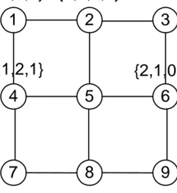
CHAPTER 2. BACKGROUND WORK 9 1 2 3 4 5 6 7 8 9 Source Destination {0,0,2,2} {2,1,0,1} {1,0,1,2} {0,1,2,1}
Figure 2.1: 3x3 2D Grid Sensor Network Topology
efficient topology construction and routing. In some other systems, the sensor nodes cannot be placed pre-deterministically, however the location of the base station can be determined a priori. In that case the location of the base station also has a great impact on the performance of the system.
Directional Source-Aware Routing Protocol (DSAP): Ayad et al. [15] proposes
power aware routing protocol for the sensor networks where the locations of the sensor nodes can be determined. They also explore different topologies to find out the optimum one. Authors incorporate power considerations into routing tables. In DSAP, each node has a unique identifier set. Each number in the set corresponds to the number of nodes separating it from the edge of the network in a particular direction. For example in a 3x3 2D-Grid network shown in Figure 2.1, node 1 has identifier {0,0,2,2}. For that node the number of neighboring nodes in left and up direction is 0, but in bottom and right direction it is 2. Whenever a node wants to send data to another node, their identifiers are subtracted. The positive values gives information about the direction of the data. After that, among different possibilities in that direction the closest node to the destination is chosen as next hop.
For instance suppose that node 1 wants to send data to node 6. Their respective identifiers are {0,0,2,2} and {2,1,0,1} (identifier is in format left,up,right,down). Once we subtract the second from the first we get {-2,-1,2,1}. When we omit the negative values we get that the destination node is
CHAPTER 2. BACKGROUND WORK 10
at right-down direction. The possible neighbors for forwarding are node 2 and node 4. The closest to the destination is node 4 and the data is forwarded to it. The routing continues until the data reaches to the destination node.
Base Station Positioning: In systems where the number and the locations of base
stations can be determined a priori it is also important to use this flexibility in order to achieve good lifetimes. Bogdanov et al. [3] showed that the number and locations of the base stations has a great impact on network lifetime. The main goal in their work is to maximize data rate. Therefore, firstly they propose a method for finding the maximum-rate routing based on maximum flow problem when the number and the locations of the base stations are given. It is also shown that optimizing the number and locations of base stations is NP-complete even in very well structured network topologies. So, they run different search algorithms for finding the optimal layout of the base stations.
2.3
Routing in Sensor Networks
As mentioned in Chapter 1, sensor networks are a new family of wireless networks whose performance metrics are different than any other networks such as mobile ad-hoc networks or cellular networks. Therefore routing algorithms proposed for wireless networks so far do not meet the requirements of sensor networks. For a good network layer protocol for sensor networks the power efficiency is the most important issue.
First aspect of the power efficiency is the power efficient routes. This is about the metrics that must be used while finding the most efficient route among the alternatives. We will explain these in detail in the following section.
Another aspect is data aggregation. Since the nodes close to each other sense the same event, dispatching the sensed data separately more than once is an energy waste. The same events must be detected and aggregated as soon as possible. Also data aggregation can also be perceived as methods for combining data coming from different sensor nodes into a set of meaningful information. In
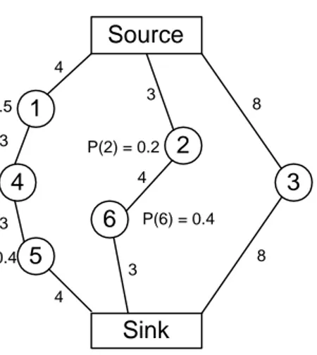
CHAPTER 2. BACKGROUND WORK 11 Source Sink 3 2 6 1 4 5 P(3) = 0.7 P(2) = 0.2 P(6) = 0.4 P(1) = 0.5 P(4) = 0.3 P(5) = 0.4 8 8 3 4 3 4 3 3 4
Figure 2.2: A sample sensor network
this point of view data aggregation is known as data fusion.
2.3.1
Routing Metrics
In order to define the routing metrics we have to mention about the parame-ters of the system. In sensor networks there are two main parameparame-ters: remain-ing power available of node i: P (i), and the cost of the transmission between nodes i and j: C(i, j). First one is a cost function related to nodes, whereas the second one is related to the links between the nodes. A sample sensor network is depicted in Figure 2.2. The numbers on the links are the corresponding cost of the transmission over that link.
There are different metrics proposed for efficient routes. We will investigate four popular ones. We will explain these on the network given in Figure 2.2.
• Minimum Hop Routing (MH): This routing metric chooses the path with
minimum number of nodes between the source and sink. In our network this route is <source,3,sink>. This metric do not consider any parameters. Only goal is to shorten the route in terms of hops. This metric can be useful when the cost of forwarding a packet is much more than the cost of directly
CHAPTER 2. BACKGROUND WORK 12
sending it to the furthest node in the range.
• Maximum Available Power Routing (MAP): The path with maximum total
available power is the MAP route. Total available power of a path is calcu-lated as the sum of the available powers of the nodes on that path. Accord-ing to this metric the optimum route in our network is <source,1,4,5,sink>. By using this metric we can prolong the lifetime of the system, since this metric chooses the nodes with highest available power. However, this ap-proach lengthens the path in terms of hops and increases the power con-sumption of the route, especially after some significant amount of time. This is because it does not consider the transmission costs of the links.
• Minimum Transmission Energy Routing (MTE): The route with minimum
total transmission energy is preferred in this metric. Minimizing the sum of the transmission costs of the links on the path between source and sink gives MTE route. <source,2,6,sink> route is optimum when we use this metric. For a packet delivery the minimum possible energy consumption throughout the system can be achieved by this metric. However, if the same source-sink pair has a great amount of data to exchange compared with other pairs, the nodes on the MTE route will drain off their energies quickly.
• Maximum-minimum Available Power Routing (MMAP): The route which
is maximum among alternatives in terms of the minimum available power on the routes. The minimum power node on a route is the cost of the route. The route which maximizes this cost between source and destination is selected. In our example the MMAP route is <source,3,sink>. This metric also considers only the available power parameter. Therefore total transmission cost can not be optimized. MMAP routing, however, prevents a low power node to be used up much earlier than others.
In a work by Toh [20], the performances of these metrics are compared via simulation. Toh also proposes a new routing metric in order to simultaneously satisfy both objectives: to maximize the lifetime, and to distribute the power consumption evenly among the nodes.
CHAPTER 2. BACKGROUND WORK 13
2.3.2
Routing Algorithms
There are several routing algorithms designed for the wireless ad-hoc networks [17, 19]. Not all of them are directly applicable to sensor networks. We will investigate some of the mostly used methods and especially which are related with our work.
Flooding: Flooding is an old method that can be used for routing in sensor
net-works. It is a simple algorithm that requires no complex topology maintenance or route discovery algorithms. In this method, every node that receives a packet broadcasts it to its neighbors. If some predetermined number of hops is travelled the packet is dropped regardless of whether the packet is reached to the destina-tion or not. It is not an efficient technique since it does not consider any energy parameters of the system.
Gossiping: This algorithm is an improvement over flooding [6]. Instead of
broad-casting a packet, each node selects a random neighbor and forwards the packet to it. It solves the poroblem of having multiple copies of the same packet, however it takes longer to find a route. It is also again not a power efficient method.
Sensor Protocols for Information via Negotiation (SPIN): Heinzelman et al. [7]
propose a family of adaptive protocols called SPIN. Main goal of SPIN is to remove the deficiencies of flooding technique by negotiation. The algorithm is based on two observations: sensor nodes can operate more efficiently when they send data that describes data (meta-data),which is very small compared to actual data, and they must monitor the changes in their energy levels.
SPIN works by using three types of messages instead of the data itself: ADV, REQ, and DATA. ADV is the advertisement message. It includes the meta-data of a data that is received from another node or that is sensed. REQ message is the request for the data advertised. DATA message is the actual measured data. Whenever a node obtains data it advertises it by using ADV message. Each node receiving ADV message checks whether it needs the data or not. The node which needs the actual data sends back a REQ message indicating the request. After that the DATA is sent to the node that requested it. The node that receives the
CHAPTER 2. BACKGROUND WORK 14
DATA packet again broadcasts an ADV message, and as a result the interested nodes in entire network receives the DATA packet.
Directed Diffusion: Directed diffusion proposed by Intanagonwiwat et al. [9] is a
data dissemination paradigm for sensor networks. In this paradigm, different from previous ones, the sink nodes (base stations) broadcast their interest to all sensor nodes for some specific event. The interest packet is simply a task descriptor. Each sensor node caches the interest locally and sets up several gradients from the source back to the sink. Gradient is direction state created in each node that receives the interest. By using gradients one can find multiple paths from source to the sink. Whenever a node has data for the specified interest, it sends it to the sink node following the multiple gradient paths. The network reinforces one or a small number of these paths.
The protocols, which we have discussed so far, was reactive protocols in which the route is established only when two nodes wants to communicate. At any time nodes do not know the route to the base station. They have to find a route specific for themselves whenever they have data to send. The cost of finding a route is, however, expensive since it generally involves a flooding operation. They are usually good for low/medium traffic networks. However, when the traffic is high reactive protocols perform poor. For such systems proactive protocols must be employed. Proactive protocols maintain routes to all other nodes in the system. Therefore the routes are known for each node regardless of whether the node has data to send or not. Regular route updates must be performed in order to keep the system running efficiently. The following two protocols are examples for proactive routing protocols.
Low Energy Adaptive Clustering Hierarchy (LEACH): In environments where the
sensor nodes periodically sense and generate data to be sent to the base station, it is important to minimize the total energy spent by the system in order to achieve long network lifetime. LEACH is proposed by Heinzelman et al. [8] for such systems. It is assumed that base station is far away from the field of in-terest, so directly communicating with it is a very costly operation. In LEACH, the key idea is to reduce the number of nodes communicating directly with the
CHAPTER 2. BACKGROUND WORK 15
base station. The protocol achieves this by forming a small number of clus-ters in a self-organizing manner, where each cluster-head collects the data from nodes in its cluster, fuses and sends the result to the base station. LEACH also uses randomization in cluster-head selection and achieves a significant amount of improvement compared to the direct transmission approach where each node directly transmits its data to the base station.
Power Efficient Gathering in Sensor Information Systems (PEGASIS): Lindsey
and Raghavendra [10] propose PEGASIS which is an improvement over LEACH for the same scenario. PEGASIS reduces the number of nodes communicating directly with the base station to one by forming a chain passing through all nodes where each node receives from and transmits to the closest possible neighbor. The data is collected starting from each endpoint of the chain until the randomized head-node is reached. The data is fused each time it moves from node to node. The designated head-node is responsible for transmitting the final data to the base station.
Chapter 3
System Model and Problem
Specification
In this chapter we will investigate the environment of the system in details. The system model is mainly the same as in [8, 10]. We present energy analysis for different protocols and reasonings yielding our protocols.
3.1
Radio Model
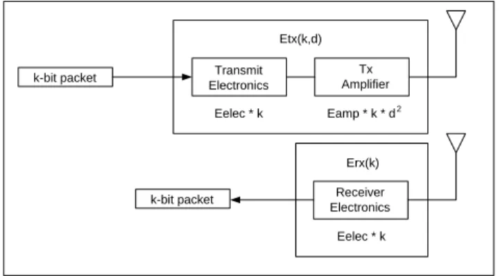
Recently, there is a significant amount of work in the area of building low-energy radios. In our work, we used the first order radio model presented in [8] (Fig-ure 3.1). In this radio model, the energy dissipation of the radio in order to run the transmitter or receiver circuitry is equal to Eelec = 50nJ/bit, and to run the transmit amplifier it is equal to Eamp = 100pJ/bit/m2. It is also assumed an
d2 energy loss due to channel transmission. Therefore, the energy expended to transmit a k-bit packet to a distance d and to receive that packet with this radio model is:
ET x(k, d) = Eelec∗ k + Eamp∗ k ∗ d2 (3.1)
ERx(k) = Eelec∗ k (3.2)
CHAPTER 3. SYSTEM MODEL AND PROBLEM SPECIFICATION 17 Transmit Electronics Tx Amplifier Receiver Electronics Eelec * k Eamp * k * d2 Etx(k,d) Erx(k) Eelec * k k-bit packet k-bit packet
Figure 3.1: First order radio model
It is also assumed that the radio channel is symmetric, which means the cost of transmitting a message from A to B is the same as the cost of transmitting a message from B to A.
As mentioned in [8], the energy required for receiving a message is not so low. Therefore, the routing protocols must also minimize the number of receive and transmit operations for a specific node while minimizing the transmit distances. It is also important to note that the cost of one transmission of a k-bit packet to the system is either:
Cij(k) = 2 ∗ Eelec∗ k + Eamp∗ k ∗ d2ij (3.3)
or
C0
i(k) = Eelec∗ k + Eamp∗ k ∗ d2ib (3.4)
where Cij is the cost of transmission between node i and node j, Ci0 is the cost between node i and the base station, dij is the distance between node i and node
j, and dibis the distance between node i and the base station. Since Ci0 is smaller than Cij when the term with Eamp is much smaller than the term with Eelec, for the overall system lifetime it can be advantageous to increase the number of transmissions to the base station.
The parameter values used in our work are the same as those used in LEACH and PEGASIS, in order to see the level of energy savings that our protocols can
CHAPTER 3. SYSTEM MODEL AND PROBLEM SPECIFICATION 18
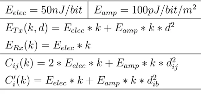
Table 3.1: Parameter values for radio model
Eelec = 50nJ/bit Eamp = 100pJ/bit/m2
ET x(k, d) = Eelec∗ k + Eamp∗ k ∗ d2 ERx(k) = Eelec∗ k Cij(k) = 2 ∗ Eelec∗ k + Eamp∗ k ∗ d2ij C0 i(k) = Eelec∗ k + Eamp∗ k ∗ d2ib achieve.
The parameters, their values, and the formulations are summarized in Ta-ble 3.1.
3.2
Problem Statement
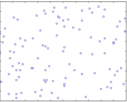
In this work, our main consideration is wireless sensor networks where the sensors are randomly distributed over an area of interest. Figure 3.2 shows a 100-node sensor network on an area of size 50 m x 50 m. The locations of sensors are fixed and the base station knows them all a priori1. The sensors are in direct communication range of each other and can transmit to and receive from the base station. The nodes periodically sense the environment and have always data to send in each round (period) of communication. The nodes aggregate or fuse the data they receive from the others with their own data, and produce only one packet regardless of how many packets they receive.
The problem is to find a routing scheme to deliver data packets collected from sensor nodes to the base station, which maximizes the lifetime of the sensor network under the system model given above. However, the definition of the lifetime is not clear unless the kind of service the sensor network provides is given. In applications where the time that all the nodes operate together is
1This information can be entered manually to the base station, or the base station can get the coordinates from the nodes if the nodes are equipped with GPS, or alternatively techniques like triangulation can be used.
CHAPTER 3. SYSTEM MODEL AND PROBLEM SPECIFICATION 19 0 10 20 30 40 50 60 70 80 90 100 0 10 20 30 40 50 60 70 80 90 100
Figure 3.2: A random 100-node sensor network on a field of size 100 m x 100 m.
important, – since the quality of the system will be dramatically decreased after first node death – lifetime is defined as the number of rounds until the first sensor is drained of its energy. In another case, where the nodes are densely deployed, the quality of the system is not affected until a significant amount of nodes die, since adjacent nodes record identical or related data. In this case, the lifetime of the network is the time elapsed until half of the nodes or some specified portion of the nodes die. In general, the time in rounds where the last node depletes all of its energy defines the lifetime of the overall sensor network. Taking these different possible requirements under consideration, our work gives timings of all deaths for all algorithms in detail and leaves the decision which one to choose to system designers.
3.3
Energy Analysis for Data Routing
In [8], the energy dissipations in MTE (Minimum-Transmission-Energy) routing and direct transmission are compared and it is figured out that an ideal system
CHAPTER 3. SYSTEM MODEL AND PROBLEM SPECIFICATION 20
Figure 3.3: Chain based routing scheme on a sample network.
must use a hybrid of both when the base station is far away from the nodes. The authors propose a two-level clustering hierarchy based routing scheme, in which the number of nodes (cluster-heads) that transmit data to the base station is reduced to 5%, while all of other nodes determine their closest gateway (cluster-head) to the base station in order to send their data. The cluster-heads are chosen randomly in order to make the system lifetime longer. However, since this algorithm is purely random, it is far from optimal.
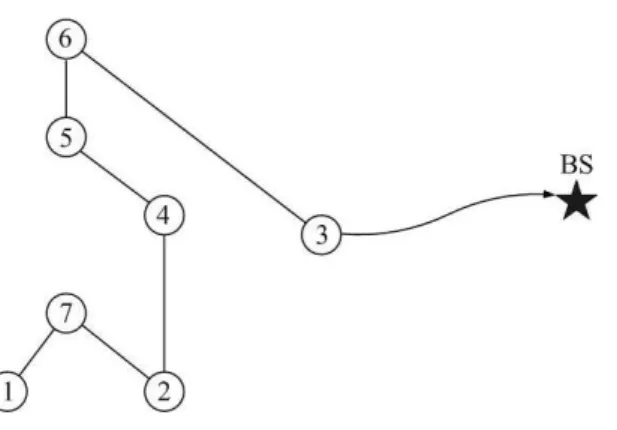
In [10], authors noticed that in a close neighborhood, the cost of running re-ceive or transmit circuitry is larger than the cost of running the amplifier circuitry for a single node. So they propose a scheme where all nodes receive and transmit only once over the edges of a chain passing through all nodes and whose length is close to minimum. In each round, a special node is selected randomly to send the fused data to the base station. Thus, only one node communicates with the base station. The algorithm works fine when the base station is far away from the field in which case the cost of sending data to the base station is almost the same for all nodes. In that case, regardless of who sends data to the base station, for a round of communication the algorithm tries to minimize the energy consumed by each node, in turn maximizes the lifetime of the nodes. Figure 3.3 shows a routing scheme that [10] computes for a sample network.
However, when the base station is inside the field (close to the center), both of the protocols perform poor. This is mainly because they do not take the exact
CHAPTER 3. SYSTEM MODEL AND PROBLEM SPECIFICATION 21
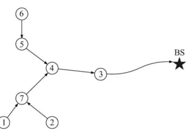
Figure 3.4: Minimum spanning tree based routing scheme on a sample network.
cost of sending data to base station into account and make a decision according to that. In addition to this, the approaches so far have not considered minimizing the total energy consumed per-round in the system.
We believe that the main idea, in order to maximize the network lifetime, should be to minimize the total energy expended in the system in a round of communication, while balancing the energy consumption among the nodes.
The first part of the idea can be realized optimally by computing a minimum spanning tree over the sensor network with link costs Cij (given in Equation 3.3)
among the nodes and C0
i (given in Equation 3.4) between the nodes and base station. The data packets are then routed to the base station over the edges of the computed minimum spanning tree. We call this routing strategy as PEDAP. Figure 3.4 illustrates the idea on a sample network.
Although PEDAP does not take the balancing issue into account, it always achieves a good lifetime for the last node. This is because, until the time the first node dies, the minimum possible energy is expended from the whole system. So the total remaining energy is optimum for the rest of the nodes. This is true for each death, thus after each node death the remaining energy in the system is maximum. So PEDAP protocol achieves almost the optimum lifetime for the last node in the system, while providing a good lifetime for the first node.
CHAPTER 3. SYSTEM MODEL AND PROBLEM SPECIFICATION 22
b) a)
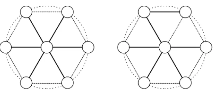
Figure 3.5: The conditions when an Euclidian MST has maximum node degree of a) six, b) five.
more it receives from others, the more energy it consumes. So while achieving total minimum energy throughout the system we must consider the degrees of the nodes. Fortunately, any euclidian minimum spanning tree has a maximum node degree of six. Figure 3.5.a shows this very rare condition. Moreover it is known that for a given point set in a plane there is always an MST of degree at most five [11]. For instance in Figure 3.5.b shows that MST constructed by connecting two neighboring nodes on the circle, and deleting the corresponding edge between the node at the center and one of the nodes. However, our case is not exactly an euclidian MST. Fortunately, in our case the only nodes that can have degree of more than 5 are the base stations. So minimum spanning tree approach realizes a quite good balance.
In order to achieve a better balance of the load (henceforth the energy con-sumption) among the nodes, we can use the information about the remaining energy of each node. When the base station is far away from the nodes, the node that dies first is usually the one that sends aggregated and fused data to the base station. So, a node with low remaining energy would not want to send to the base station. That node would like to expend its remaining energy by sending to a nearby neighbor and thus try to maximize its lifetime. Also a low-energy node would not like to receive many packets from others, since receiving is a high cost operation as well. Its tendency would be only to send its data and not to receive anything from others. In order to achieve these, a slight change in the
CHAPTER 3. SYSTEM MODEL AND PROBLEM SPECIFICATION 23
cost functions helps us. The new cost functions will be as follows:
Cij(k) = 2 ∗ Eelec∗ k + Eamp∗ k ∗ d2ij ei (3.5) C0 i(k) = Eelec∗ k + Eamp∗ k ∗ d2ib ei , (3.6)
where ei is the remaining energy of node i, which is normalized with respect to the maximum possible energy in the battery (i.e. 0 ≤ ei ≤ 1).
As it can be noticed, now the cost of communication between the nodes is not symmetric. According to Equation 3.5, the cost of sending a message from a node i to its neighbors increases as the remaining energy of node i decreases. Although this new formula usually does not change the selection of the neighbor which a node sends, it postpones the inclusion of that node in the spanning tree. The later a node is included in the spanning tree, the fewer number of messages it will receive. According to Equation 3.6, for a low-energy node the cost of sending to the base station is increased, and thereby the willingness to send to the base station for that node is decreased. So, if the minimum spanning tree algorithm would be executed periodically every certain number of rounds (such as 100), a more power efficient routing scheme is found for the next period, depending on the current situation (the nodes that are alive and their energy levels). This is the idea behind the power-aware version of PEDAP, which we will call PEDAP-PA (Power Efficient Data gathering and Aggregation Protocol - Power Aware).
CHAPTER 3. SYSTEM MODEL AND PROBLEM SPECIFICATION 24 0 10 20 30 40 50 60 70 80 90 100 0 10 20 30 40 50 60 70 80 90 100
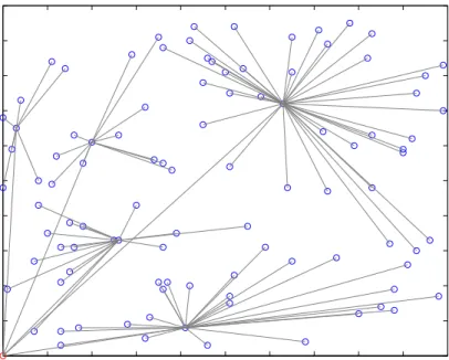
Figure 3.6: Routing paths for a sample network - LEACH. Base station is at (0,0). 0 10 20 30 40 50 60 70 80 90 100 0 10 20 30 40 50 60 70 80 90 100
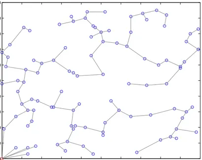
Figure 3.7: Routing paths for a sample network - PEGASIS. Base station is at (0,0).
CHAPTER 3. SYSTEM MODEL AND PROBLEM SPECIFICATION 25 0 10 20 30 40 50 60 70 80 90 100 0 10 20 30 40 50 60 70 80 90 100
Chapter 4
PEDAP Algorithm Details
In this chapter, we consider firstly the basic environment for implementing our algorithms in a real-life situation. After that, we discuss other environments where our algorithms are also feasible to implement.
In this work, we assume that all nodes and base station are in direct com-munication range of each other. This means there is no bound for maximum transmission distance for any of the nodes. We also do not consider the length of a round in time. This is reasonable for applications where the measurements are taken infrequently such as periodic measurements of average temperature in an area of interest.
PEDAP algorithm can be divided into two phases: setup phase and commu-nication phase. The following sections give details of the phases.
4.1
Setup Phase
The PEDAP protocols are both centralized algorithms where the base station is responsible for computing the routing information. This is because, in systems where some elements are resource limited whereas one or more elements are pow-erful, it is desirable to give the computation load to the more powerful elements
CHAPTER 4. PEDAP ALGORITHM DETAILS 27
of the system.
In setup phase several tasks are handled. One of them is collecting information about the nodes. The other is computing efficient routes centrally. The last task that must be accomplished is to inform the nodes about the routes.
Information Collection
Since PEDAP protocols are centralized algorithms, some information about the nodes must be collected by the base station in order to compute the routes. Most important information is the transmission costs of each sensor node pairs. However collecting this is not feasible. So the locations of the nodes can be used to approximate the actual costs according to radio model given in Chapter 3. In some systems the locations of the sensor nodes are predetermined. If this is the case, the locations of the nodes can be loaded to the base station either in hardware or in software. Another way of finding out the locations is to ask to the nodes about their locations if the nodes are equipped with GPS (Global Positioning System). If this is also not possible, sophisticated methods such as triangulation can be used.
For implementing PEDAP-PA accurately at base station we need also the remaining energy levels of all the nodes. Base station can estimate them using the radio model given, however actually the physical system is time varying. The power exponent is usually not always 2. In order to handle this, in last round of the communication phase (i.e. 100th) all nodes send their remaining energy levels. Since this information is very small compared to the actual data, no significant amount of energy is consumed for that. We assume that the batteries of the nodes are initially full.
Efficient Route Computation
Once the locations of the nodes is retrieved somehow, the routing information is computed using Prim’s MST algorithm [13] where base station is the root. The algorithm works as follows: Initially, we put a node in the tree which is the base station in our case. After that, in each iteration we select the minimum weighted
CHAPTER 4. PEDAP ALGORITHM DETAILS 28 0 10 20 30 40 50 60 70 80 90 100 0 10 20 30 40 50 60 70 80 90 100
Figure 4.1: Routing paths of sample network.
edge from a vertex in the tree to a vertex not in the tree, and add that edge to the tree. In our case this means that the vertex just included in the tree will send its data through that edge. We repeat this procedure until all nodes are added to the tree. The details are given in Algorithm 4.1. In Figure 4.1, the resulting routing paths are illustrated for a sample network. Since we choose linear array implementation for priority queue, the running time complexity of our algorithm is O(n2) assuming there are n nodes in the network. If we use binary heap implementation, complexity becomes O(n2log(n)) since the corresponding graph is complete.
In order to implement PEDAP-PA, only change that must be made is to change the cost functions. The algorithm works fine for two protocols.
As seen, the base station is included in the network graph. Thus, by com-puting a minimum spanning tree over this graph with the cost functions given as above and by routing packets according to that spanning tree, we achieve a minimum energy consuming system.
CHAPTER 4. PEDAP ALGORITHM DETAILS 29
Algorithm 1 Route Computation Algorithm for each sensor s do
distance[s] ← C0 s parent[s] ← BASE end for Q ← all sensors while Q 6= Ø do s ← EXTRACT-MIN(Q)
for each sensor p in Q do if Csp< distance[s] then parent[p] ← s distance[p] ← Csp end if end for end while Informing Nodes
After a power efficient routing scheme is computed, it must be informed back to the sensor nodes. In order to do that base station sends each node necessary information about that node, such as the node’s parent in the tree in order to reach to the base station; the time slot number when the node will send its data to its parent in a round; from how many different neighbors the node will receive packets in a round and when, etc.
So, the cost of setting-up the system with the new routing information is equal to only the sum of costs of running the receiver circuitry of each node. Therefore, the set-up cost for periodically establishing the scheme is very small compared to LEACH and PEGASIS.
4.2
Communication Phase
We divided each round into stages whose length is equal to the time to send a message multiplied by the maximum in-degrees of the minimum spanning tree. The number of stages is determined by the depth of the tree. In the first stage, all leaf nodes at maximum depth send their data to their parents. The parents apply
CHAPTER 4. PEDAP ALGORITHM DETAILS 30
TDMA (Time Division Multiple Access) scheme among their children. Each node sends its message with its parents CDMA (Code Division Multiple Access) code, in order to prevent collisions with the messages of other nodes sending to different parents at the same time. In the next stages, the procedure climbs one level up until it reaches the root, the base station.
After a predetermined number of such rounds all nodes stop sending their data, and turn on their receivers to get the information about the new routing paths computed by the base station. This number is an important parameter for our protocols. There is a tradeoff about this number. If this number is small, the routing paths are more sensitive to the changes in the system (node deaths, remaining energy levels). However, if this number is kept small, the time for setup phase dominates the communication phase. So we choose 100 rounds for this parameter.
Our protocols can also work in environments where all the nodes and the base station are not in direct communication range of each other. In this case, a distributed minimum spanning tree algorithm [5] can work. However, this method increases set-up cost dramatically. On the other hand, if the base station can still transmit to all the nodes directly and has the location information about all nodes, the scheme can be efficiently computed at the base station assuming the visibility graph is given.
For the two protocols proposed in this work, the route computation algorithm is the same. Only thing that must be changed is the cost functions. So switching between the two proposed protocols requires only a small change in the base station and no changes in sensor nodes. This makes our protocols preferable when different applications with different lifetime requirements will be executed in the same sensor network from time to time.
Chapter 5
Experimental Results
In order to evaluate the performance of our algorithms, we simulated five different routing schemes: Direct transmission, LEACH, PEGASIS, PEDAP and PEDAP-PA, the later two being our proposals. The simulations are done in C. We generate networks of diameters 50 m and 100 m randomly, each having 100 nodes. We repeated the simulations for the same network twice: one with a distant base station, other with a base station in the center. We located the base station to point (0, −100) in simulations where it is distant. We ran the simulations with different network sizes and different initial energy levels. The aim was to determine the timings of node deaths (in terms of rounds) until the last node dies. Once a node dies, we consider it dead for the rest of the simulation. We re-computed the routing information every 100 rounds for all algorithms. This parameter is important for the actual system performance. A small value leads better results for all algorithms. However, in that case the set-up costs, which are not included in the simulations, may dominate the communication costs.
Figures 5.1 and 5.2 show the timings of all deaths for networks whose diame-ters are 50 m and 100 m respectively and where the base station is far away from the field. As seen, while LEACH and direct transmission perform far from opti-mal, PEGASIS provides a good improvement in both cases. However, PEDAP-PA further improves the lifetime of the first node about 400%, while providing almost the same lifetime for the last node, compared with PEGASIS. On the other hand,
CHAPTER 5. EXPERIMENTAL RESULTS 32 0 10 20 30 40 50 60 70 80 90 100 0 500 1000 1500 2000 2500 3000
Number of Node Deaths
Time (rounds) direct leach pedap pegasis pedap−pa
Figure 5.1: Timings of node deaths in a network of size 50 m x 50 m - The base station is distant from the field.
0 10 20 30 40 50 60 70 80 90 100 0 500 1000 1500 2000 2500 3000
Number of Node Deaths
Time (rounds) direct leach pedap pegasis pedap−pa
Figure 5.2: Timings of node deaths in a network of size 100 m x 100 m - The base station is distant from the field.
CHAPTER 5. EXPERIMENTAL RESULTS 33
compared again with PEGASIS, PEDAP improves the lifetime of the last node about 25%, while providing almost the same lifetime for the first node.
Figures 5.3 and 5.4 provide the same information, but in this case the base station is located in the center of the field. Now, both PEDAP and PEDAP-PA improve the lifetime of the last node about two times compared with PEGASIS and LEACH. The improved value is the same as it is in direct transmission, which is optimum. As for the first node death time, both PEDAP protocols improve it when compared with others. However, PEDAP-PA achieves about two times improvement over PEDAP. Therefore, we can conclude that PEDAP-PA is the best performing algorithm for systems where base station is in the center of the field. It gives the best lifetime for the first node, while providing the optimum lifetime for the last. However, if the nodes are not power-aware, PEDAP is a good alternative for the same environment.
Figure 5.5 shows the total remaining energy in the system with time, when the base station is far away from the field; and Figure 5.6 shows the total remaining energy in the system with time, when the base station is in the center of the field. The plots show that the energy dissipations per round in PEDAP protocols are always near to optimal. PEGASIS is closer to the optimum when the base station is far away. On the other hand, direct transmission is closer to the PEDAP protocols when the base station is in the center of the field.
Tables 5.1 and 5.2 summarize the results for two different base station loca-tions and for three different initial energy levels in a network of diameter 100 m. In these tables, FND and LND stand for the times at which the first and the last node die. HND stands for the time at which half of the nodes die. Note that the performance of LEACH is very close to direct communication in all simulations. This is because we recompute the routing information every 100 rounds, which is a reasonable number. So, LEACH protocol consumes too much energy until 100th round.
Also it is worth to note that doubling initial energy level almost doubles the lifetimes in all protocols as expected. In PEDAP-PA, however, when the initial energy is doubled, the lifetime of first node increases about 2.5 times. We believe
CHAPTER 5. EXPERIMENTAL RESULTS 34 0 10 20 30 40 50 60 70 80 90 100 0 500 1000 1500 2000 2500 3000 3500 4000 4500 5000
Number of Node Deaths
Time (rounds) direct leach pedap pegasis pedap−pa
Figure 5.3: Timings of node deaths in a network of size 50 m x 50 m - The base station is in the center.
0 10 20 30 40 50 60 70 80 90 100 0 500 1000 1500 2000 2500 3000 3500 4000 4500 5000
Number of Node Deaths
Time (rounds) direct leach pedap pegasis pedap−pa
Figure 5.4: Timings of node deaths in a network of size 100 m x 100 m - The base station is in the center.
CHAPTER 5. EXPERIMENTAL RESULTS 35 0 500 1000 1500 2000 2500 3000 0 5 10 15 20 25 Time (rounds) Total energy direct leach pedap pegasis pedap−pa
Figure 5.5: Total remaining energy in the system as time passes - The base station is distant from the field.
0 500 1000 1500 2000 2500 3000 3500 4000 4500 5000 0 5 10 15 20 25 Time (rounds) Total energy direct leach pedap pegasis pedap−pa
Figure 5.6: Total remaining energy in the system as time passes - The base station is in the center.
CHAPTER 5. EXPERIMENTAL RESULTS 36
that this is because PEDAP-PA finds more chance to recompute the routing information with increasing initial energy. As the number of re-computations increases, more energy saving routing paths are achieved, since PEDAP-PA is power-aware unlike others.
CHAPTER 5. EXPERIMENTAL RESULTS 37
Table 5.1: Comparison of timings of node deaths in terms of number of rounds under different protocols. Base station is in the center. FND, HND, and LND stand for first node death, half of the nodes death, and last node death.
Energy(J) Protocol FND HND LND DIRECT 596 1147 4836 LEACH 297 1247 2223 0.25 PEGASIS 439 2259 2667 PEDAP 1228 2334 4836 PEDAP-PA 2177 2352 4836 DIRECT 1192 2293 9672 LEACH 1036 2927 4362 0.50 PEGASIS 774 4496 5175 PEDAP 2455 4668 9672 PEDAP-PA 4353 4688 9672 DIRECT 2383 4586 19343 LEACH 2627 5603 7747 1.00 PEGASIS 1428 9036 10443 PEDAP 4910 9336 19343 PEDAP-PA 8705 9378 19343
CHAPTER 5. EXPERIMENTAL RESULTS 38
Table 5.2: Comparison of timings of node deaths in terms of number of rounds under different protocols. Base station is distant from the field. FND, HND, and LND stand for first node death, half of the nodes death, and last node death.
Energy(J) Protocol FND HND LND DIRECT 61 104 223 LEACH 60 255 632 0.25 PEGASIS 184 1856 2190 PEDAP 213 2135 2674 PEDAP-PA 998 2103 2217 DIRECT 121 208 445 LEACH 123 661 2134 0.50 PEGASIS 1070 3767 4344 PEDAP 426 4271 5337 PEDAP-PA 2897 4067 4272 DIRECT 242 416 889 LEACH 351 1983 3961 1.00 PEGASIS 1332 7309 8536 PEDAP 851 8544 10665 PEDAP-PA 6899 7763 8438
Chapter 6
Conclusion and Future Work
In this thesis, we investigate the wireless sensor network systems, where periodic measurements are taken by the sensor nodes and where these data must be sent to the base station. The data is fused or aggregated on the way to the base station. The sensor nodes have limited energy. So, the main objective is to maximize the lifetime of the network.
In this work, we present PEDAP and PEDAP-PA, two power efficient data gathering and aggregation protocols based on minimum spanning tree routing scheme. We show through simulations that our protocols perform well. PEDAP outperforms previous approaches, LEACH and PEGASIS, by constructing min-imum energy consuming routing for each round of communication. PEDAP-PA takes it further and tries to balance the load among the nodes. Minimizing the total energy of the system while distributing the load evenly to the nodes has a great impact on system lifetime. This is confirmed through simulations.
Our simulations show that if keeping all the nodes working together is impor-tant, PEDAP-PA performs best among others, regardless of the position of the base station. On the other hand, if the lifetime of the last node is important or the nodes are not power-aware, PEDAP is a good alternative.
It is worth to note that our protocols also perform well when the base station 39
CHAPTER 6. CONCLUSION AND FUTURE WORK 40
is inside the field. There have been no approaches so far for this scenario except direct transmission.
Our simulation results showed that the location of the base station has a great impact on the network lifetime. Intuitively, we can see that the number of the base stations will also influence the lifetime. A comprehensive research can be done on the effect of these parameters to the lifetime of the system as a future work.
The distributed version of our protocols can also be studied. The key issues are the time required for constructing the routes, and the energy dissipation per node in setup phase. This work is important for systems where the locations of the nodes can not be determined, or base station can not reach all the nodes.
Another interesting work can be done on the same scenario, however in this case sensor nodes have a maximum transmission distance. So, the nodes will not be in direct communication range of each other. The visibility graph must be used when calculating the routing paths. The effect of PEDAP-PA will obviously be reduced, however it remains as a question that whether it will still improve the lifetime or not.
Bibliography
[1] I. F. Akyildiz, W. Su, Y. Sankarasubramaniam, and E. Cayirci. Wireless sensor networks: a survey. Computer Networks, 38(4):393–422, 2002.
[2] M. Bhardwaj, A. Chandrakasan, and T. Garnett. Upper bounds on the lifetime of sensor networks. In IEEE International Conference on
Commu-nications, pages 785–790, 2001.
[3] A. Bogdanov, E. Maneva, and S. Riesenfeld. Power-aware base station posi-tioning for sensor networks. In Proceedings of INFOCOM 2004. To appear. [4] B. Chen, K. Jamieson, H. Balakrishnan, and R. Morris. Span: An energy-efficient coordination algorithm for topology maintenance in ad hoc wireless networks. In Proceedings of the 7th ACM International Conference on Mobile
Computing and Networking, pages 85–96, Rome, Italy, July 2001.
[5] R. G. Gallager, P. A. Humblet, and P. M. Spira. A distributed algorithm for minimum-weight spanning trees. ACM Transactions on Programming
Languages and Systems, 5(1):66–77, January 1983.
[6] S. Hedetniemi, S. Hedetniemi, and A. Liestman. A survey of gossiping and broadcasting in communication networks. Networks, 18(4):319–349, 1988. [7] W. Heinzelman, J. Kulik, and H. Balakrishnan. Adaptive protocols for
in-formation dissemination in wireless sensor networks. In MOBICOM, pages 174–185, 1999.
[8] W. R. Heinzelman, A. Chandrakasan, and H. Balakrishnan. Energy-efficient communication protocol for wireless microsensor networks. In 33rd Annual
BIBLIOGRAPHY 42
Hawaii International Conference on System Sciences,, pages 3005 – 3014,
2000.
[9] C. Intanagonwiwat, R. Govindan, and D. Estrin. Directed diffusion: a scal-able and robust communication paradigm for sensor networks. In Mobile
Computing and Networking, pages 56–67, 2000.
[10] S. Lindsey and C. S. Raghavendra. Pegasis: Power-efficient gathering in sensor information systems. In IEEE Aerospace Conference, March 2002. [11] C. Monma and S. Suri. Transitions in geometric minimum spanning trees
(extended abstract). In Proceedings of the seventh annual symposium on
Computational geometry, pages 239–249. ACM Press, 1991.
[12] T. Pering, T. Burd, and R. Brodersen. The simulation and evaluation of dy-namic voltage scaling algorithms. In Proceedings of International Symposium
on Low Power Electronics and Design, pages 76–81, August 1998.
[13] R. Prim. Shortest Connecting Networks and Some Generalizations. Bell
Syst. Tech. J., 36:1389–1401, 1957.
[14] P. Rentala, R. Musunuri, S. Gandham, and U. Saxena. Survey on sensor networks. Technical Report UTDCS-10-03, University of Texas at Dallas, 2003.
[15] A. Salhieh, J. Weinmann, M. Kochhal, and L. Schwiebert. Power efficient topologies for wireless sensor networks. In Proceedings of the International
Conference on Parallel Processing, pages 156–163.
[16] C. Schurgers, V. Tsiatsis, and M. B. Srivastava. Stem: Topology manage-ment for energy efficient sensor networks. In Aerospace Conference 2002, March 2002.
[17] S. Singh, M. Woo, and C. S. Raghavendra. Power-aware routing in mobile ad hoc networks. In Mobile Computing and Networking, pages 181–190, 1998. [18] A. Sinha and A. Chandrakasan. Dynamic power management in wireless
sen-sor networks. Trans. Design and Test of Computers, 18(2):62–74, Mar./Apr. 2001.
BIBLIOGRAPHY 43
[19] I. Stojmenovic and X. Lin. Power-aware localized routing in wireless net-works. IEEE Transactions on Parallel and Distributed Systems, 12(11):1122– 1133, 2001.
[20] C.-K. Toh. Maximum battery life routing to support ubiquitous mobile computing in wireless ad hoc networks. IEEE Communications Magazine, 39(6):138–147, June 2001.
[21] Y. Xu, J. Heidemann, and D. Estrin. Geography-informed energy conser-vation for ad hoc routing. In Proceedings of the ACM/IEEE International
Conference on Mobile Computing and Networking, pages 70–84, Rome, Italy,