Optical near field interaction of spherical quantum dots

OPTICAL NEAR FIELD INTERACTION OF

SPHERICAL QUANTUM

DOTS

A THESIS

SUBMITTED TO THE DEPARTMENT OF PHYSICS

AND THE GRADUATE SCHOOL OF ENGINEERING AND SCIENCE OF BILKENT UNIVERSITY

IN PARTIAL FULLFILMENT OF THE REQUIREMENTS FOR THE DEGREE OF

MASTER OF SCIENCE

By

Togay Amirahmadov

July, 2012

ii

I certify that I have read this thesis and that in my opinion it is fully adequate, in scope and in quality, as a thesis for the degree of Master of Science.

Assoc. Prof. Hilmi Volkan Demir (Supervisor)

I certify that I have read this thesis and that in my opinion it is fully adequate, in scope and in quality, as a thesis for the degree of Master of Science.

Prof. Oğuz Gülseren

I certify that I have read this thesis and that in my opinion it is fully adequate, in scope and in quality, as a thesis for the degree of Master of Science.

Assoc. Prof. Azer Kerimov

Approved for the Graduate School of Engineering and Sciences:

Prof. Levent Onural

iii

ABSTRACT

OPTICAL NEAR FIELD INTERACTION OF

SPHERICAL QUANTUM

DOTS

Togay Amirahmadov M.S. in Physics

Supervisor: Assoc. Prof. Hilmi Volkan Demir July, 2012

Nanometer-sized materials can be used to make advanced photonic devices. However, as far as the conventional far-field light is concerned, the size of these photonic devices cannot be reduced beyond the diffraction limit of light, unless emerging optical near-fields (ONF) are utilized. ONF is the localized field on the surface of nanometric particles, manifesting itself in the form of dressed photons as a result of light-matter interaction, which are bound to the material and not massless. In this thesis, we theoretically study a system composed of different-sized quantum dots involving ONF interactions to enable optical excitation transfer. Here this is explained by resonance energy transfer via an optical near-field interaction between the lowest state of the small quantum dot and the first dipole-forbidden excited state of the large quantum dot via the dressed photon exchange for a specific ratio of quantum dot size. By using the projection operator method, we derived the formalism for the transfered energy from one state to another for strong confinement regime for the first time. We performed numerical analyses of the optical near-field energy transfer rate for spherical colloidal quantum dots made of CdSe, CdTe, CdSe/ZnS and PbSe. We estimated that the energy transfer time to the dipole forbidden states of quantum dot is sufficiently shorter than the radiative lifetime of excitons in each quantum dot. This model of ONF is essential to understanding and designing systems of such quantum dots for use in near-field photonic devices.

Keywords: optical near field, dressed photon, resonance energy transfer, excitons.

iv

ÖZET

KÜRESEL KUANTUM NOKTALARININ OPTİK YAKIN

ALAN ETKİLEŞİMİ

Togay Amirahmadov Fizik Bölümü, Yüksek Lisans

Tez Yöneticisi: Doç. Dr. Hilmi Volkan Demir Temmuz 2012

Nano ölçekli malzemeler ileri fotonik cihazlar yapmak için kullanılabilir. Yeni ortaya konulan optik yakın alanlardan (OYA) faydalanılmadıkça, bilinen uzak alan ışığı kullanılarak, fotonik cihazların boyutu kırınım sınırının altına indirilemez. OYA nanometrik parçacıkların yüzeyi üzerinde yerelleşmiş, malzemeye bağlı, kütlesiz olmayan ve ışık madde etkileşimi sonucunda kendisini döşenmiş fotonlar şeklinde gösteren bir alandır. Bu tez çalışmasında, optik uyarılma transferi sağlamak için, farklı boyutlu kuantum noktalarından oluşan OYA etkileşimli bir sistemi teorik olarak inceledik. Burada, enerji aktarımı kuantum nokta boyutlarının belirli bir oranı için giyinmiş foton alışverişi yoluyla küçük kuantum noktasının taban seviyyesi ve büyük kuantum noktasının ilk uyarılmış dipol yasaklı seviyyesi arasındaki optik yakın alan etkileşimi aracılığıyla rezonans enerji aktarımı ile açıklanabilir. İzdüşüm operatörü yöntemini kullanarak, ilk kez güçlü sınırlandırma bölgesinde bir seviyyeden diğerine aktarılan enerji için gereken formalizmi türetdik. CdSe, CdTe, CdSe/ ZnS ve PbSe malzemelerinden yapılan küresel kolloidal kuantum noktaları için optik yakın alan enerji aktarım hızının sayısal analizini yaptık. Kuantum noktalarının dipol yasaklı seviyelerine enerji aktarım süresinin, kuantum noktalarında bulunan eksitonların ışınımsal ömür süresinden yeterince kısa olduğunu hesapladık. Bu OYA modeli, yakın alan fotonik cihazlarında kullanılacak kuantum nokta sistemlerinin tasarımı ve anlaşılması için çok önemlidir.

Anahtar kelimeler: Optik yakın alan, döşenmiş foton, rezonans enerji aktarımı, eksitonlar.

v

Acknowledgements

First I would like to acknowledge my advisor Assoc. Prof. Hilmi Volkan Demir. I had the opportunity to share two years of my academic life and experience with him and with our group members. I will never forget his kind attitude and

encouragement. I am thankful to him to provide me with anopportunity to work

with him and understand the first step for being a good researcher and scientist. In our group meetings I learned a lot of things from him. He is not only a good academic advisor, for me he is also a good teacher.

My special thanks go to Dr. Pedro Ludwig Hernandez Martinez for his help in my research. I cannot forget his friendship, encouragement and his optimistic way of handling problems when we faced during my research period.

Also Iwould like to thank Prof. Oğuz Gülseren and Assoc. Prof. Azer Kerimov for being on my jury and for their support and help.

Now come my friends. I would like to acknowledge our group members Burak Güzeltürk, Yusuf Keleştemur, Shahab Akhavan, Sayım Gökyar, Evren Mutlugün, Cüneyt Eroğlu, Kıvanç Güngör, Can Uran, Ahmet Fatih Cihan, Veli Tayfun Kılıç, Talha Erdem, Aydan Yeltik, Yasemin Coşkun, Akbar Alipour and Ozan Yerli for their friendship and collaboration.

Also very importantly, among the management and technical team and the post doctoral researchers of the group: Dr. Nihan Kosku Perkgoz, Ozgun Akyuz, and Emre Unal; and Dr. Vijay Kumar Sharma. I am very thankful to you all for great friendship and support.

I am thankful to the present and former members of the Devices and Sensors Demir Research Group.

I would like to acknowledge Physics Department and all faculty members, staff graduate students especially Sabuhi Badalov, Semih Kaya and Fatmanur Ünal for their support and friendship.

vi

My special thanks is for my family, especially for my father. Although he is not here with us, he would have been very happy. I am thankful to their support and encouragement despite all the difficulties. I dedicate this thesis to my father.

vii

Table of Contents

ACKNOWLEDGEMENTS ... V

1. INTRODUCTION ... 1

1.1 THE OPTICAL FAR FIELD AND DIFFRACTION LIMIT OF LIGHT ... 1

1.2 WHAT IS OPTICAL NEAR-FIELDS ... 2

2. THEORETICAL BACKGROUND OF OPTICAL NEAR FIELDS ... 6

2.1 DIPOLE-DIPOLE INTERACTION MODEL OF OPTICAL NEAR FIELDS ... 6

2.2 PROJECTION OPERATOR METHOD.EFFECTIVE OPERATOR AND EFFECTIVE INTERACTION ... 12

2.3 OPTICAL NEAR-FIELD INTERACTION POTENTIAL IN THE NANOMETRIC SUBSYSTEM ... 14

2.4 OPTICAL NEAR-FIELD INTERACTION AS A VIRTUAL CLOUD OF PHOTONS AND LOCALLY EXCITED STATES ... 18

3. OPTICAL NEAR-FIELD INTERACTION BETWEEN SPHERICAL QUANTUM DOTS ... 25

3.1 INTRODUCTION ... 25

3.2 ENERGY STATES OF SEMICONDUCTOR QUANTUM DOTS ... 26

3.3 QUANTUM CONFINEMENT REGIMES. STRONG, INTERMEDIATE AND WEAK CONFINEMENTS. ... 32

3.4 OPTICAL NEAR-FIELD INTERACTION ENERGY BETWEEN SPHERICAL QUANTUM DOTS FOR STRONG AND WEAK CONFINEMENT REGIMES ... 36

3.4.1 STRONG CONFINEMENT ... 36

3.4.2 WEAK CONFINEMENT ... 39

3.5 NUMERICAL RESULTS FOR CDTE ,CDSE,CDSE/ZNS AND PBSE QUANTUM DOTS ... 41

viii

APPENDIX A

PROJECTION OPERATOR METHOD EFFECTIVE OPERATOR

AND EFFECTIVE INTERACTION ... 61 APPENDIX B

DERIVATION OF THE INTERACTION POTENTIAL

... 66

APPENDIX C

OPTICAL NEAR FIELD INTERACTION BETWEEN QUANTUM

DOTS FOR STRONG CONFINEMENT REGIME ... 75 APPENDIX D

DERIVATION OF THE PROPE SAMPLE INTERACTION

POTENTIAL ... 83

ix

List of Figures

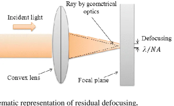
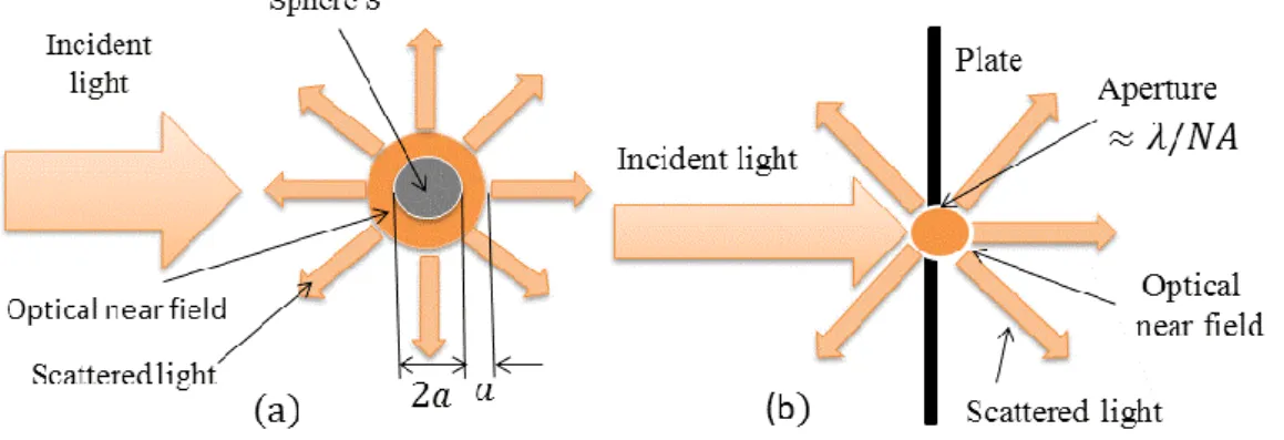
Figure 1.1.1 The schematic representation of residual defocusing.…………....1 Figure 1.2.1 The schematic representation of generation of an optical near fields (a) Generation of optical near fields on the surface of the sphere S. (b) Generation of optical near fields by a small subwavelength aperture. ………...….3

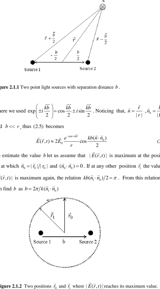
Figure 1.2.2 Generation of optical near field and electric field lines. (Taken from M. Ohtsu Principles of Nanophotonics 2008.) ... 3 Figure 1.2.3 Nanometric subsystem composed of two nanometric particles and optical near fields generated between them...5 Figure 2.1.1 Two point light sources with separation distance b.………..…....8

Figure 2.1.2 Two positions r₀ and r₁ where | ( , ) |E r t reaches its maximum value………...……….…8

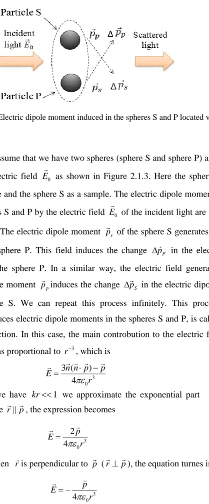
Figure 2.1.3 Electric dipole moment induced in the spheres S and P located very close to each other………...….. 10 Figure 2.2.1 The schematic representation of Pspace spanned by the eigenstates |₁and |₂ and its complementary space Q………..…. 13

Figure 2.4.1 Schematic representation of near-field optical system. rS and rP

show the arbitrary positions in sample and probe...19 Figure 2.4.2 Exchange of real and virtual exciton-polariton………..……...20

Figure 2.4.3 The system composed of QD S and P with two resonant coupled energy levels. | S and | A are correspond to symmetric and antisymmetric states... 22

x

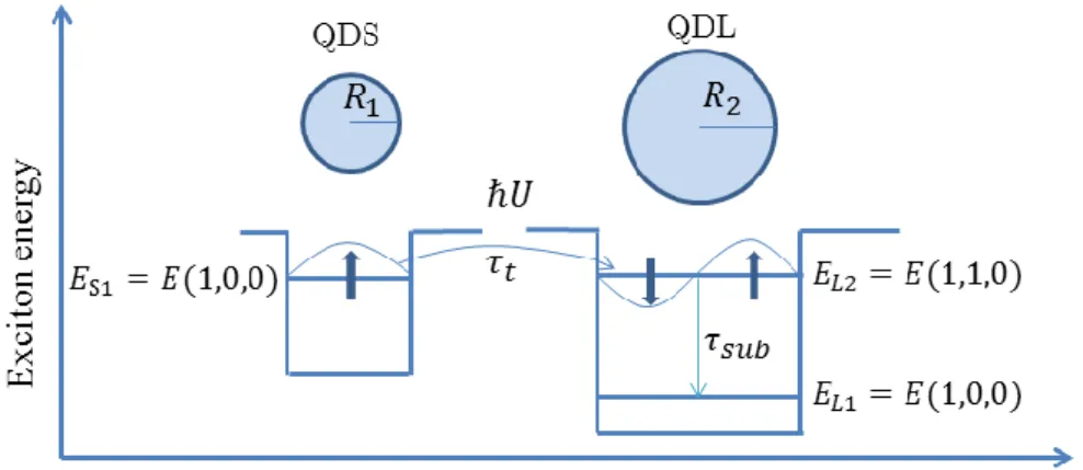
Figure 3.2.1 Band sructure and energy band gap E_g of bulk semiconductor. The diagram shows the creation of one electron-hole pair as a result of photon absorption...30 Figure 3.5.1 Optical near-field interactions between two spherical quantum dots with the size ratio of R R_{2 1}1.43.There is a resonance between ( , , )n l m (1, 0, 0)level of QDS and ( , ,n l m   ) (1,1, 0)level of QDL... 41 Figure 3.5.2 Optical near-field energy and distance relation for CdSe spherical quantum dots from ( , , )n l m (1, 0, 0)state of QDS to ( , ,n l m   ) (1,1, 0) _state

of QDL...43

Figure 3.5.3 Optical near-field transfer rate and distance relation for CdSe spherical quantum dots from ( , , )n l m (1, 0, 0)state of QDS to

( , ,n l m   ) (1,1, 0)state of QDL... 44 Figure 3.5.4 Optical near-field energy and distance relation for CdTe spherical quantum dots from ( , , )n l m (1, 0, 0)state of QDS to ( , ,n l m   ) (1,1, 0)state of QDL...44

Figure 3.5.5 Optical near-field transfer rate and distance relation for CdTe spherical quantum dots from ( , , )n l m (1, 0, 0)state of QDS to

( , ,n l m   ) (1,1, 0)state of QDL... 45 Figure 3.5.6 Optical near-field energy and distance relation for CdSe/ZnS spherical quantum dots from ( , , )n l m (1, 0, 0)state of QDS to

( , ,n l m   ) (1,1, 0)state of QDL...46 Figure 3.5.7 Optical near-field transfer rate and distance relation for CdSe/ZnS spherical quantum dots from ( , , )n l m (1, 0, 0)state of QDS to

xi

Figure 3.5.8 Optical near-field energy and distance relation for PbSe spherical quantum dots from ( , , )n l m (1, 0, 0)state of QDS to ( , ,n l m   ) (1,1, 0)state of QDL...47

Figure 3.5.9 Optical near-field transfer rate and distance relation for PbSe spherical quantum dots from ( , , )n l m (1, 0, 0)state of QDS to

( , ,n l m   ) (1,1, 0)state of QDL... 48 Figure 3.5.10 Comparison of optical near-field energy transfer for PbSe, CdSe/ZnS, CdTe and CdSe spherical quantum dots from

( , , )n l m (1, 0, 0)state of QDS to ( , ,n l m   ) (1,1, 0)state of QDL. ... 48 Figure 3.5.11 Optical near-field interactions between two cubic CuCI quantum dots with the size ratio of R R_{2 1}1.41. There is a resonance between (1,1,1)level of QD-S and (2,1,1)levels of QD-L... 50

Figure 3.5.12.a Optical near-field energy transfer for cubic CuCI quantum dots from ( ,n n n_{x y}, _z)(1,1,1)state of QDS to ( ,n n n_x   _y, _z) (2,1,1) state of QDL...51

Figure 3.5.12.b Optical near-field energy transfer rate for cubic CuCI quantum dotsfrom ( ,n n n_{x y}, _z)(1,1,1) state of QDS to ( ,n n n_x   _y, _z) (2,1,1)

xii

1

Chapter 1

Introduction

1.1 The optical far field and diffraction limit of light

One of the intrinsic characteristic of waves is diffraction. This phenomenon is explained as following. Imagine that we have a plate with very small aperture on the surface and plane light propagates on it. After the light passes through an aperture it is converted into a diverging spherical wave. This divergence is called diffraction. The divergence angle is  a for circular aperture where,  is the wavelength of an incident light and a is aperture radius. When the distance between the aperture and the plane in which the pattern is observed is large enough than the wavelength of light then, this region is often called as a far field and expressed with a distance greater than 2

4

D , where, D is the largest dimension in the aperture and -is the wavelength of the incident light.

As shown in the Figure 1.1.1 the plane wave incident on a positive lens is focused at a point by convex lens. Even if we focus the light to the convex lens due to the diffraction limit the spot size of the light cannot be zero. This phenomena is called defocusing.

2

The spot size of the light is about  NA where, NA is called the numerical aperture and usually is given as nsin. Here, n is the refractive index of the medium and the angle  is obtained from sin 

 

a 2 f2

 

a 2 2 where, f is focal length and _{a is the diameter of the lens.[2]}

The semiconductor lasers, optical waveguides and related integrated photonic devices must confine the light within them for effective operation. However, as long as conventional light is used, the diffraction limit restrict the miniaturization of the optical science and technology. Therefore, to go beyond the diffraction limit we need nonpropogating localized light that is free of diffraction. Since optical near fields is free of diffraction it has been proposed to transcend the diffraction limit of light.[1]-[4]

1.2 What is optical near fields?

The optical near felds are spatially localized fields on the surface of nanometric particles. It is generated when we excite the nanometric material by incident light. Figure 1.2.1a represents the generation mechanism of optical near fields. Here the radius a of the sphere S is assumed to be much smaller than the wavelength of incident light. In the Figure 1.2.1.a the scattered light represents the light scattered from the surface of the sphere S and corresponds to the far field light. However, as a result of light-matter interaction an optical localized field with thickness about a is also generated on the surface of the sphere S . This localized field is called optical near-field. Since it is localized on the sphere S it cannot be seperated from the sphere. The volume of this optical near field is smaller than the diffraction limited value because the size of a particle is much smaller than the wavelength of incident light a . Figure 1.2.1b represents generation of an optical near field by a small aperture. The scattered light in the figure corresponds to the far field light and propogaters to the far field. However, again the localized field around the aperture corresponds to the near fields. The decay length of near

3

field is much smaller than the wavelength of incident light and it does not depends on the wavelength. It only depends on the size of the nanometric material.

In figure 1.2.1a the thickness of the optical near field is about a . This can be explained as follow. By directing the light on the nanometric object _{S we excite} electrons in S . As a result, due to the Coulomb forces generating from the electric field of incident light, the nuclei and electrons in atoms of _{S are displaced from} their equilibrium position.

Figure 1.2.1 The schematic representation of generation of an optical near fields

(a) Generation of optical near fields on the surface of the sphere S. (b) Generation of optical near fields by a small subwavelength aperture

Figure 1.2.2 Generation of optical near field and electric field lines. (Taken from

4

Since the nuclei and electrons are oppositely charged, their displacement direction are opposite. Therefore, electric dipoles are generated on the surface of the sphere S . The product of the charge and the displacement vector of electric dipole is called the electric dipole moment. These electric dipoles are oscillated with the oscillating electric field of incident light and attract or repel each other. As a result the spatially localized electric field with thickness a is generated on the surface of the sphere. Figure 1.2.2 shows the electric field lines of the dipoles on the sphere A . Represented electric field lines on the surface of the particle A corresponds to the optical near field. As shown in this figure the electric dipole moments are connected by these electric field lines. They represent the magnitude and orientations of the Coulomb forces. These electric lines tend to take possible shortest trajectory. They emanate from one electric dipole moment and terminate at another. This is the reason why optical near fields is very thin. As shown in the Figure 1.2.2 as we move away from the surface of the particle the optical near field potential decreases rapidly and at distance _{a it becomes negligible small.} This arises from the fact that the most of the electric field lines are located on a close distances to the surface of a particle. The two kinds of electric field lines is shown in Figure 1.2.2. One is the electric lines of the optical near field which are at close proximity to the surface of particleA . The other force lines which form a closed loop correspond to the far field.

Figure 1.2.3 represents the nanometric and macroscopic subsystems. Nanometric subsystem consists optical near field and two particles. The macroscopic subsystem consists of the electromagnetic fields of scattered light incident light and substrate material. Since the optical near fields localized on the surface of the particle it does not carry energy to the far field, therefore it can not be detected. In order to detect the optical near fields the second particle P is placed near the particle S . By placing the particle P close to the near field of the particle S some of the force lines of the near field of the sphere S is directed to the surface of P and induces electric dipole moments on P. By this way, the near field of the particle S is disturbed by the particle P and disturbed near field is converted to the propogating light and its transferred energy can be detected by the photodetector.

5

Figure 1.2.3 Nanometric subsystem composed of two nanometric particles and optical near fields generated between them.

Here the two particles are considered interacting with each other by exchanging the exciton-polariton energies. Since the local electromagnetic interaction happens in a very short amount of time, the exchange of virtual exciton-polariton energies is allowed due to uncertainty principle. Optical near fields mediates this interaction, that is represented by Yukawa type function. [1]-[6] In the following chapters the theoretical background of the optical near fields and the numerical analysis for the energy transfer rate for different quantum dots is discussed. The organization of the rest of this thesis is given as following:

In Chapter 2 the theoretical background of optical near fields is presented. The near field conditions is shown and the dipole-dipole interaction model is described. By using the projection operator method the effective near field interaction potential is derived and the nature of the optical near field is described as a virtual cloud of photons.

In Chapter 3 the optical near field energy transfer is explained. The equation for the transfered energy from one state to another is derived for strong and weak confinement regime. The numerical analysis of the optical near-field energy transfer rate for spherical CdSe, CdTe, CdSe/ZnS and PbSe quantum dots was made. Finally, in Chapter 4 summarizing the thesis the application of the theory is briefly discussed.

6

Chapter 2

Theoretical Background of Optical

Near Fields

2.1 Optical near field as a dipole-dipole interaction

model

Let us investigate the optical near-field interaction in a viewpoint of dipole-dipole interaction model. For simplicity let us assume two separate nanometric particles with seperation distance R and charge densities 1 and 2. In this case the Coulomb interaction energy between these two nanometric object is given by

3 3 1 1 2 2 12 1 2 0 1 2 ( ) ( ) 1 4 | | r r V d r d r r r     



(2.1)

If we assume that the extent of the charge distributions 1 and 2 is much smaller than their seperation R, we can expand the interaction potential V₁₂ in a multiple series as 2 1 2 1 2 2 1 1 2 1 2 12 3 3 5 0 ( ) ( ) ( ) 3( )( ) 1 ( ) 4 q q q p R q p R R p p p R p R V R R R R R           _     _   (2.2)

where R r2 r1, and the multipole and dipole moments of the charge is defined as q



( )r d r 3  and p



( )r r d r  3 , respectively. Here the first term of expansion is the charge-charge interaction and it spans over along distances since the distance dependence is R1. The next two terms correspond to the charge dipole interaction and has a distance dependence of R2. Therefore, it has a shorter range than the first term. The fourth term shows the dipole-dipole interaction and decays with R3. It is the most important interaction among neutral particles and strongly depends on the dipole orientations. This term gives

7

rise to Van der Waals forces and Förster-type energy transfer. In a similar way, the electric field vector can be given by [12],[33]





2 2 3 0 1 1 1 ( ) 3 ( ) 4 ikr ik E k n p n n n p p e r r r        _   _{ }   _  _       (2.3)

Since the magnitude of the first term is larger for kr >>1, it represents the component dominating in the far field region. In contrast, the third term represents the electric field component that dominates in the close proximity of

pbecause it is the largest when kr <<1.

Now let us assume two point light sources. The separation distance between these two sources is b and it is assumed to be the size of material object as shown in Figure 2.1.1. The vector r represents the seperation distance between the object and the detection point S. Since we can treat the two particles as a point light source, the electric field E r t( , ) at time t and the position r can be defined as a superposition of the electric field vectors of the two point light sources

| 2| | 2| 0 0 ( , ) | 2 | | 2 | i t ik r b i t ik r b m m e e E r t E E r b r b             (2.4)

where E is the electric field vector of incident light, ₀ 2 is the angular frequency and k2  is the wave number. The quantity k r| b 2 |represents the phase delay t. Here depending on the values of b and r, we can consider three possible cases.

Case 1. 1 << kb << kr

In this case, since 1<<kb, the term proportional to r1 in (2.3)is larger than the other terms and, hence, the value of m should be one. Therefore, (2.4)

approximates to

( , ) ₀ cos sin ₀ cos sin

2 2 2 2 | 2 | | 2 | i t ikr i t ikr e kb kb e kb kb E r t E i E i r b r b     _{ }   _{ }  _  _ _  _  _{ }  _{ } (2.5)

8

Figure 2.1.1 Two point light sources with separation distance b.

where we used exp cos sin

2 2 2 kb kb kb i i          . Noticing that, | | r n r  , | | b b n b 

and b << r_, thus (2.5) becomes 0 ( ) ( , ) 2 cos 2 i t ikr b kb n n e E r t E r    _  (2.6)

To estimate the value b let us assume that | ( , ) |E r t is maximum at the position 0

r at which n₀ |r₀| |r₀| and (n n₀ _b)0. If at any other position r₁ the value of

| ( , ) |E r t is maximum again, the relation kb n n( ₁ _b) 2 . From this relation we can find b as b2 k n n( ₁ _b)

9

Case 2. kb <<1 << kr

In this case, since kb << kr again, the value of m in (2.4) takes unity. To estimate b from (2.6), the inequality kb n n|  b| 2  should be satisfied. In other

words the phase difference between the light waves of the two light sources has to be larger than  at the detection point. Since we have |n n _b | 1 , the requirement above changes to kb2 . This condition represents the diffraction limit of light. However, since kb <<1 this requirement cannot be met and, therefore, the value of b cannot be obtained. In other words, since the phase difference between the two light waves is sufficiently small, we cannot measure the sub-wavelength-sized object at the detection point r in the far field.

Case 3. kb < kr << 1

In this case, since kr1, the terms in (2.3)proportional to r1 and r2are very small and, thus, the term proportional to 3

r dominates. Therefore, we choose 3

m . Also, since the phase delay k r| b 2 | is sufficiently small, (2.4)

approximates to 0 _{3 3} 1 1 ( , ) | 2 | | 2 | i t E r t E e r b r b      _  _     (2.7)

If we assume that the electric field amplitude at point r₀ is |E and ₁| r0 is normal to the vector b , then the value b is derived from relation (n n0 b)0 as

1 2 2 3 2 0 0 1 2 | | 2 | | E b r E _{ }     _{ }  _{ }    (2.8)

From this relation, we find E to be 1

3 2

2 2

1 0 0

|E | 2 | E | _r ( 2)b _ . It means that we can determine the value of b by the near field measurement. To conclude, the relation kbkr1 _{is called the near field condition and the range of} rsatisfying this condition kr1is called the near field.

10

Figure 2.1.3 Electric dipole moment induced in the spheres S and P located very close to

each other.

Now let us assume that we have two spheres (sphere S and sphere P) and incident light with electric field E as shown in Figure 2.1.3. Here the sphere P can be 0 used as probe and the sphere S as a sample. The electric dipole moments induced in the spheres S and P by the electric field E of the incident light are ₀ pp and ps

respectively. The electric dipole moment p_s of the sphere S generates an electric field in the sphere P. This field induces the change p_P in the electric dipole moment of the sphere P. In a similar way, the electric field generated by the electric dipole moment p_pinduces the change p_S in the electric dipole moment of the sphere S. We can repeat this process infinitely. This process, which mutually induces electric dipole moments in the spheres S and P, is called dipole-dipole interaction. In this case, the main controbution to the electric field comes from the terms proportional to r3, which is

3 0 3 ( ) 4 n n p p E r     (2.9)

Here since we have kr1 _{we approximate the exponential part} ikr

e to 1. When we take r|| p, the expression becomes

3 0 2 4 p E r   (2.10)

Similarly, when ris perpendicular to p (r  p), the equation turnes into [2],[32] 3 0 4 p E r    (2.11)

11

Equations (2.10) _and (2.11) represent the optical near field generated around the spheres S and P. If we assume that the spheres S and P are dielectric, the electric dipole moment p_s induced by the incident electric field E is ₀

0

S S

p  E

(2.12) Here _Sis the polarizability of the dielectric.

In the near field case, if the conditions kR1 and R|| pare satisfied, the electric field generated in the sphere P by the electric dipole moment p_s can be written as

3 0 2 4 S S p E R   (2.13)

Therefore, we can write the change in the electric dipole moment of the sphere P as 0 3 0 2 4 P S P P S p E E R        (2.14)

Since we can represent the change in the dipole moment as   p_P _PE₀, the change in the polarizability of the sphere P can be given as

3 0 2 P S P R       (2.15)

where _S and _P are 3

i g ai i   and 0 0 0 4 2 i i i g       

 for (i=S,P), aS and aP are

the respective radii, and_S and _P are the electric constants of the spheres S and P, respectively. If we replace the role of the spheres S and P, the discussion above will be still valid. The electric dipole moment p_P _PE₀ will generate the electric field EP2pP 40R3in the sphere S and induce the change   pS SE0 in the electric dipole moment. Therefore, _S and _P takes the same value as

3 0 2 P S S P R             (2.16)

Since in the near field condition (kR1) we assume that the two spheres are very close to each other, they can be recognized as a single object for the far-field detection. Therefore, the intensity I_S of the scattered light generated from the total electric dipole moment p_P  p_P p_S  p_S is

12 2 | ( ) ( ) | S P P S S I  p  p  p  p (2.17) Taking into account that pS SE0 and   pS SE0, we have

2 2 2 0 0 ( ) | | 4 ( ) | | S S P S P I    E     E (2.18)

Here the first term (_S _P) |2 E₀|2corresponds to the intensity of the light scattered directly by the spheres S and P, whereas the second term

2 0

4 ( S P) |E | represents the intensity of scattered light as a result of dipole-dipole interaction. From the equation above, we obtain [2]

3 3 3 0 2 P S P S g g R       (2.19)

Relation 2.19 shows that the optical near field intensity strongly depends on the size of the spheres.

2.2 Projection operator method, relevant nanometric

irrelevant macroscopic subsystems, P and Q spaces

We can use the projection operator method to derive effective interaction in the nanometric material system illuminated by an incident light. This type of interaction is called optical field interaction. It is estimated that optical near-field interaction potential between the nanometric objects with a separation distance R _{is given as a sum of Yukawa potentials}

exp( R) R     (2.20) Here 1

represents the range of the interaction and corresponds to the characteristic size of nanometric material system. It depends on the size of the nanomaterial and does not depend on the wavelength of the incident light.

1



13

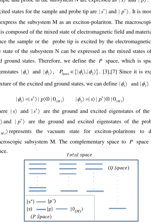
On the basis of projection operator method, we can investigate the formulation of the optical near-field system. In order to describe optical near-field interaction in a nanometric system, we think of the relevant nanometric subsystem N and irrelevant macroscopic subsystem M. The macroscopic subsystem M is mainly composed of the incident light and the substrate. The subsystem N is composed of the sample, the probe tip, and the optical near-field. To describe the quantum mechanical state of matter in the subsystems N and M, the energy states of the sample and probe in the subsystem N are expressed as | s and | p. The relevant excited states for the sample and probe tip are | sand | p. It is most reasonable to express the subsystem M as an exciton-polariton. The macroscopic subsystem M is composed of the mixed state of electromagnetic field and material excitation. Since the sample or the probe tip is excited by the electromagnetic interaction, the state of the subsystem N can be expressed as the mixed states of the excited and ground states. Therefore, we define the P space, which is spanned by the eigenstates |₁ and |₂, PSpace



| 1,| 2



. [3],[7] Since it is expressed as a mixture of the excited and ground states, we can define |₁

and |2 as

|₁   |s | p | 0_(M) |₂  |s |p| 0_(M) (2.21)

where | s and | s are the ground and excited eigenstates of the sample and

| pand | p are the ground and excited eigenstates of the probe tip. Here ( )

| 0_M represents the vacuum state for exciton-polaritons to describe the macroscopic subsystem M. The complementary space to P space is called Q

space.

Figure 2.2.1 The schematic representation of Pspace spanned by the eigenstates 1

14

In Figure 2.2.1 we have the schematic representation of P and its complementary space Q. The complementary Q space is spanned by a huge number of basis that is not included in Pspace. This method of description is called projection operator method.

The projection operator method is used to describe the quantum mechanical approach of the optical near-field interaction system that is nanometric materials surrounded by the incident light. The reason why |1and |2 contain the vacuum state | 0is to introduce the effect of the subsystem (M) by elimimating its degree of freedom. This treatment is useful to derive consistent expression for the magnitude of effective near-field interaction potential between the elements of the subsystem (N). As a result of this approach, the subsystem (N) can be treated as an independent system that is regarded to be isolated from the subsystem (M). [1],[3].

2.3 Optical near-field interaction potential in the

nanometric subsystem

By using projection operator method, we can evaluate effective interaction inP

space, which is derived in Appendix B, as

1 2 1 2

ˆ ₍ ˆ ˆ _{) (} ˆ ˆˆ ₎₍ ˆ ˆ ₎

eff

V  PJ JP  PJ VJP PJ JP  

(2.22) This result gives us an effective interaction potential of the nanometric subsystem N, which can be found in Appendix A. The Hamiltonian for the interaction between a sample or a probe and electromagnetic fields as a dipole approximation can be expressed as





ˆ ˆ ˆ ˆ ˆ _{( ) ( )} s s p p V    D r  D r (2.23)

The electric dipole operator is denoted by  ˆ (_ s p, ), where the subscript s and

15

respectively. rsand rpare the vectors representing the position of the sample and

and the tip, respectively; Dˆ( )r is the transverse component of the quantum mechanical electric displacement operator . Dˆ( )r can be expressed in terms of the photons creation a kˆ ( )

 

and annihilation ˆ ( )a k_ operators as follows





1 2 2 1 2 ˆ _{ˆ ˆ} ( ) k ( ) ( ) ikr ( ) ikr k D r i e k a k e a k e V              _{ }   



(2.24)

where k is the wavevector, _kis the angular frequency of photon, V is the quantization volume in which electromagnetic fields exist and e k_( )is the unit

vector related to the polarization direction of the photon. [34] Since exciton-polariton states as bases are employed as the bases to describe the macroscopic subsystem M, the creation and annihilation operators for photon can be replaced with the creation and annihilation operators of exciton-polariton. Therefore, after replacing photons creation and annihilation operators with exciton-polaritons and substituting ˆ_s _s( ( )B rˆ _ B rˆ( ))_ into(2.24), we can change the notation from photon base to exciton-polariton base as







1 2 2 _{ˆ ˆ} ˆ p ˆ_{( )} ˆ _{( ) ( ) ( ) ( ) ( )} s k V i B r B r K k k K k k V        _  _      _{ }    



(2.25)

Here ˆ( )B r_ and ˆ ( )B r _ denote the annihilation and creation operators for the

electronic excitation in the sample or probe ( s p, ) _and K k_( ) is the coefficient of the coupling strength between the exciton-polariton and the nanometric subsystem N and it is given by

2 1 ( ) ( ( )) ( ) ikr K k e k f k e        



 (2.26) we define f k( ) as 2 2 2 2 2 ( ) ( ) 2 ( ) ( ) ( ) ck k f k k ck k          (2.27) ( )k

 and are the eigenfrequencies of both exciton-polariton and electronic excitation of the macroscopic subsystem M. [10],[31]

16

The amplitude of effective probe-tip interaction exerted in the nanometric subsystem can be defined as

2 ˆ 1

(2,1) | |

eff eff

V   V 

(2.28) In order to derive the explicit form of effective interaction V_eff(2,1), the initial and final states (|1 |s |p | 0(M)



     and |2 |s |p | 0(M)



     ) are employed in

Pspace before and after interaction. The appoximation of ˆJ to the first order is (see Appendix B for derivations) given by

0 0 1 0 0 1 2 1 2 1 2 1 0 0 0 0 1 2 ˆ ˆ ˆ ˆ (2,1) | ( ) | | ( ) | 1 1 ˆ ˆ | | | | eff P Q P Q m P Qm P Qm V PVQV E E P P E E VQVP PVQ m m QVP E E E E                       _  _    



(2.29) where 0 P

E and E are eigenvalues of the unperturbed Hamiltonian _Q0 H in ˆ0 Pand

Q spaces. The equation shows that the matrix element m Q E| ( _P0E_Q0)1VPˆ |₁

represents a virtual transition from the initial state |₁ in Pspace to the intermediate state | m in Q space and 2|PVQ mˆ |  represents the virtual transition from the intermediate state | m in Q space to the final state |₂ in

Pspace. So, we can transform (2.10) to the following equation (please refer to Appendix B) 3 2 0 0 ( ) ( ) ( ) ( ) 1 (2,1) (2 ) ( ) ( ) ( ) ( ) p s s p eff K k K k K k K k V d k k s k p                    



(2.30)

where the summation over k is replaced by k -integration, which is 3 3 (2 ) k V d k  



_

and E_s  ₀( )s and E_p  ₀( )p are the excitation energies

of the sample (between | sand | s) and the probe tip (between | p and | p), respectively. Similarly, the probe-sample interaction Veff(1, 2)can be written as

17 3 2 0 0 ( ) ( ) ( ) ( ) 1 (1, 2) (2 ) ( ) ( ) ( ) ( ) s p p s eff K k K k K k K k V d k k p k s                    



(2.31)

The total amplitude of the effective sample-probe tip interaction can be defined as the sum of Veff(1, 2) and Veff(2,1)

2 3 2 2 , 1 3 , , , 1 ( ) ( ) ( ) ( ) ( ) ( ) 4 ( ) ( ) ( ) ( ) ( ) ( ) eff s p s p ikr ikr eff eff s p V r d k r e k r e k f k e e d k V r V r E k E E k E                         _  _{ }  _      _{ }  _ _  _  _  

 



(2.32) where 2 ( ) ( ) 2 m pol k E k E m

  is the eigenenergy of exciton-polariton and mpol is

effective mass of polariton. The integration gives us the following result

2 , 2 3 2 2 3 ( ) 1 1 ( ) ( ) 2 ( ) 3 1 3 ˆ ˆ ( )( ) 2 r eff f s p r s p V r W e r r r r r W e r r r                               _  _   _             _   _       (2.33) where 1 2Epol(Em E ) c      and W_{ } is defined as 2 2 2 ( )( ) 2 pol m m m pol m E E E W E E E E E E E            (2.34)

After summing up and taking the angular average of (_srˆ)(_p rˆ) ( _{s p}) 3, we have 2 2 , ( ) ( ) ( ) ( ) 3 r r A B eff s p e e V r W W r r                       _    _  



(2.35)

Equation(2.35)shows effective near-field interaction potential in the nanometric subsystem. The effective near-field interaction is expressed as a sum of Yukawa

functions ( r) e  r r

  

   with a heavier effective mass   (shorter

18

part of the interaction comes from the mediation of massive virtual photons or polaritons and this formulation indicates a “dressed photon” picture in which as

result of light-matter interaction, photons are not massless but

massive[1],[2],[3],[7]-[10]

2.4 Optical near-fields as a virtual cloud of photons

and locally excited states

To investigate the behavior of optical near field in a viewpoint of virtual photons let us first calculate probe sample interaction potential V_eff( , )p s

3 2 0 0 ( ) ( ) ( ) ( ) 1 ( , ) (2 ) ( ) ( ) ( ) ( ) p s s p eff K k K k K k K k V p s d k k s k p        _  _        



(2.36)

If we consider two infinitely deep potential wells with the widths a_p and as, the

eigenenergies of sample and probe are given as

2 2 0 3 ( ) 2 eS S s m a      _{ }   (2.37, )a 2 2 0 3 ( ) 2 _{eP P} p m a      _{ }   (2.37, )b

Where m_eS and m_ePare the effective masses of electron in the sample and probe. Since the coefficient K k_( ) is expressed as

2 1 ( ) ( ( )) ( ) ikr K k e k f k e        



 , the

effective sample probe interaction is then

2 ( ) 2 3 1 2 2 ₂ 2 ( ) 2 3 1 2 ₂ ( ( ))( ( )) 1 ( , ) (2 ) ₃ 2 2 ( ( ))( ( )) 1 (2 ) ₃ 2 2 p s s p ik r r s p eff p eS S ik r r s p p eS P e k e k f e V p s d k k m m a e k e k f e d k k m m a          _    _        _{  }      _{ }      _{   }     _ _{  }                  









2                _{ }    (2.38)

19

Defining heavy and light effective masses as _ and _ where we have

1 2 2 2 3 P 2 P eS P m m m a      _  _   1 2 2 2 3 P 2 P eS S m m m a      _  _   (2.39) Therefore (2.38) changes to









( ) ( ) 2 , 3 2 2 2 2 2 2 1 1 ( ( ))( ( )) (2 ) 2 2 p s s p ik r r ik r r p s eff s p p p e e V d k e k e k f k k m m                        _{   }     





(2.40)

where we approximate some of the terms as a constant and take f k( ) as f . In Figure 2.4.1 the positions given by rS and rP represent the arbitrary positions

in the sample and probe, respectively, and the position vector is defined as

| _{P S} |

r  r r . The integration of complex integral with respect to k gives us the following result for V_eff( , )p s (refer to Appendix D for derivations)

3 , 1 exp( ) exp( ) 1 ( , ) ( ) 2 exp( ) exp( ) eff si pj ij i j r i r V p s r r r i r r r                _  _      



(2.41)

and ( , ) exp( P P) exp( S S) eff i r a r a V p s r r      (2.42)

Figure 2.4.1. Schematic representation of near-field optical system. r_S and r_P show the arbitrary positions in sample and probe.

20 where 3 P P eP m m   , 3 S S eS m m   (2.43)

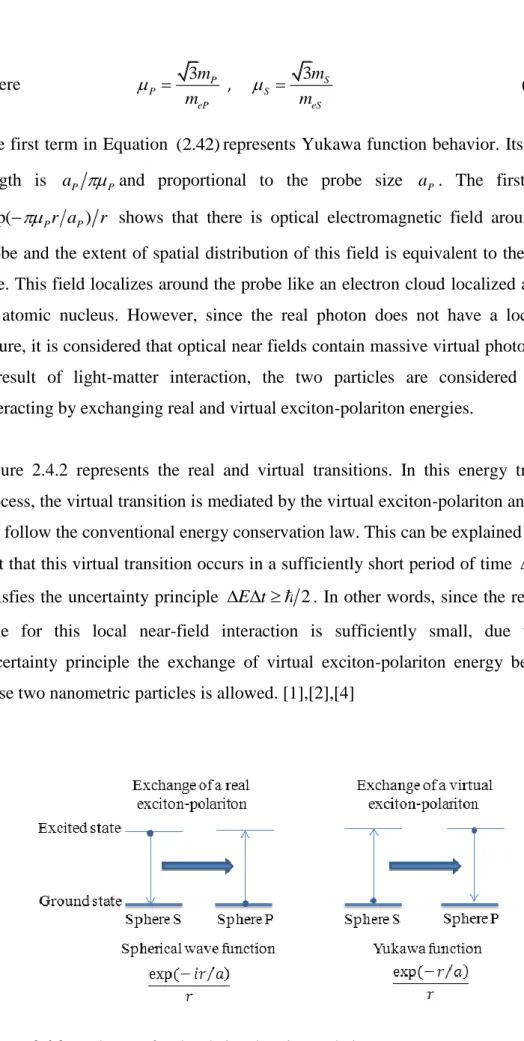
The first term in Equation (2.42)represents Yukawa function behavior. Its decay length is a_P _P and proportional to the probe size a_P. The first term

exp(_Pr a_P) r shows that there is optical electromagnetic field around the probe and the extent of spatial distribution of this field is equivalent to the probe size. This field localizes around the probe like an electron cloud localized around an atomic nucleus. However, since the real photon does not have a localized nature, it is considered that optical near fields contain massive virtual photons. As a result of light-matter interaction, the two particles are considered to be interacting by exchanging real and virtual exciton-polariton energies.

Figure 2.4.2 represents the real and virtual transitions. In this energy transfer process, the virtual transition is mediated by the virtual exciton-polariton and does not follow the conventional energy conservation law. This can be explained by the fact that this virtual transition occurs in a sufficiently short period of time t _and satisfies the uncertainty principle   E t 2. In other words, since the required time for this local near-field interaction is sufficiently small, due to the uncertainty principle the exchange of virtual exciton-polariton energy between these two nanometric particles is allowed. [1],[2],[4]

21

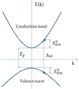
When the quantum dot is excited by propogating light, the conventional classical electrodynamics explains that an electric dipole at the center of QD is induced and the electric field generated from this electric dipole is detected in the far-field region. However, in a quantum theoretical view, the electron in the quantum dot is excited from the ground state to an excited state due to the interaction between the electric dipole and electric field of the propogating light, which is called electric dipole transition. It is assumed that two anti paralel electric dipoles are induced in a quantum dot and the electric field generated by one electric dipole is cancelled by the other in the far field region and thus the transition from the excited state cannot take place. Then the transition and excited state are said to be dipole forbidden [2].

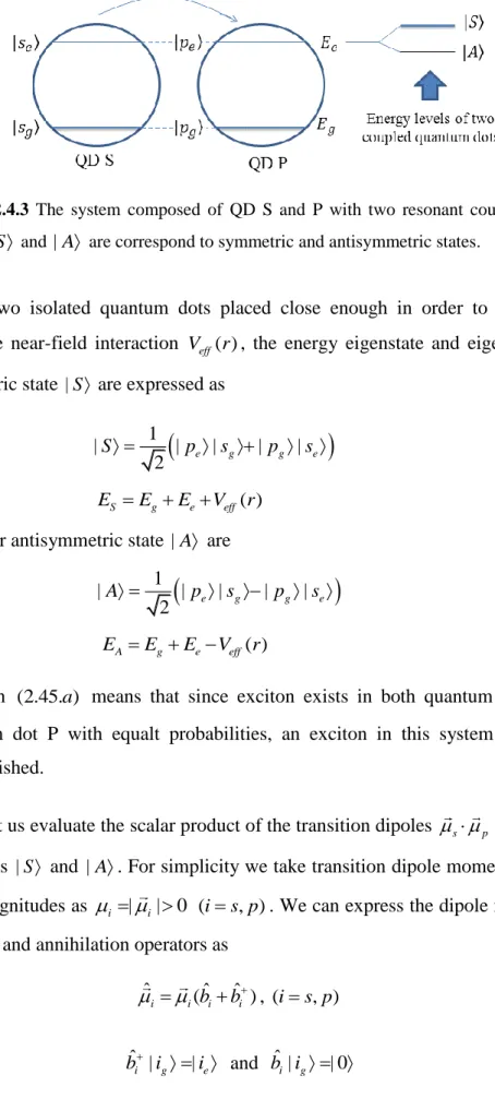
Figure 2.4.3 illustrates the system composed of two coupled quantum dots with two arbitrary resonantly coupled energy levels. These two resonant energy levels are coupled as a result of the near field interaction and as a result of this coupling, the quantized energy levels of exciton are split in two parts. One half of them corresponds to the symmetric state of the exciton, and the other half corresponds to the antisymmetric state of the exciton in the quantum dot. These two symmetric and antisymmetric states correspond to the paralel and antiparalel electric dipole moments that is induced in these relevant quantum dots.[1],[2],[11].

The ground and excited states of exciton in quantum dot S are expressed as |s_e

and |s_g. Similarly, the ground and excited states in quantum dot P are expressed as | p_eand |p_g. The energy eigenvalues of the excited states |s_e and |p_e are expressed as Ee while the energy eigenvalues of the ground states |sg and |pg

is E_g. Since they have the equal energy eigenvalues, the states |s_e and | p_e also

|s_g and | p_g are said to be in resonance with each other.

The Hamiltonian of this two level system is expressed as following

0 int

ˆ ˆ ˆ

H H H (2.44)

22

Figure 2.4.3 The system composed of QD S and P with two resonant coupled energy

levels. | S and | A are correspond to symmetric and antisymmetric states.

When two isolated quantum dots placed close enough in order to induce the effective near-field interaction V_eff( )r , the energy eigenstate and eigenvalue for symmetric state | S are expressed as





1 | | | | | 2 e g g e S  p  s  p  s  (2.45. )a ( ) S g e eff E E E V r (2.45. )b

while for antisymmetric state | A are





1 | | | | | 2 e g g e A  p  s  p  s  (2.46. )a E_AE_g E_eV_eff( )r (2.46. )b

Equation (2.45. )a means that since exciton exists in both quantum dot S and quantum dot P with equalt probabilities, an exciton in this system cannot be distinguished.

Now, let us evaluate the scalar product of the transition dipoles  _s _p in terms of the states | S and | A. For simplicity we take transition dipole moments parallel with magnitudes as _i |_i| 0 (is p, ). We can express the dipole moment by creation and annihilation operators as

ˆ ₍ˆ ˆ ₎ i i bi bi  _{ }  , (is p, ) (2.47) where ˆ |_{i g} | _e b i   i and b iˆ |_{i g}  | 0 (2.48)

23 therefore we have













ˆ ˆ ˆ ˆ | | | | | | ( )( ) | | | | 2 ˆ ˆ ˆ ˆ | | | | | | | | 0 2 s p s p e g g e s s p p e g g e s p e g s p e g g e s p g e s p S S s p s p b b b b p s p s s p b b p s s p b b p s                                        | _{s p}| _{s p} 0 S   S        (2.49)

It indicates that the transition dipole moments s and p are paralel in

symmetric state | S. Similarly for antisysmmetric state | A we have

| _{s p}| _{s p} 0

A   A  

      (2.50)

and shows that they are antiparalel in antisymmetric state. It follows from equations (2.49) and (2.50) that excitation of quantum dots with far field light leads to the symmetric state with paralel dipoles produced in QDs S and P. In contrast the near-field excitation of QDs can produce either one or both of the symmetric and antisymmetric states. Therefore, the symmetric state is called the bright state and antisymmetric state is called the dark state. This is one of the major differences between the near-field and far-field excitations. In particular locally excited states can be created in this two level system. These locally excited states can be expressed by a linear combination of symmetric and antisymmetric states as [1],[2],[5],[6],[7]





1 | | | | 2 e g p  s   S A (2.51. )a | | 1



| |



2 g e p  s   S A (2.51. )b

The right-hand terms of (2.51. )a and (2.51. )b describes the coupled states via an optical near-field. Here, the optical near-field excites both of the coupled states. However, in the far field excitation the only symmetric state is excited. The state vector |( )t  at time t is 1 | ( ) exp | exp | 2 S A iE t iE t t S A    _ _ _   _ _ _       (2.52)

24

where the state vectors |( )t are also normalized and at t0 |(0) |pe|sg

and

( ) ( )

|( )t  exp_iEt_cos_Veff r t_|p_e|s_g isin_Veff r t_| p_g|s_e_

       (2.53) 2 S A g e E E E  E E (2.54)

Then the occupation probability that the electrons in QD-P occupy the excited and the electrons in QD-S occupy the ground state is expressed as

2 2 ( ) | | || ( ) | cos e g eff p s g e V r t s p t        _ _   (2.55) Similarly, the occupation probability that the electrons in QD-P accupy the ground and the electrons in QD-S occupy the excited state is expressed as

2 2 ( ) | | || ( ) | sin g e eff p s e g V r t s p t        _ _   (2.54)

The equations (2.55) and (2.54) shows that the probability varies periodically with period of T  Veff( )r . It means that the excitation energy of the system is

periodically transfered between the coupled resonant energy levels of QD-S and QD-P. This process is called nutation.

25

Chapter 3

Optical Near Field Interaction between

Spherical Quantum Dots

3.1

Introduction

There are three regimes of confinement introduced depending on the ratio of the cristallite radius R to the Bohr radius of electrons, holes, and electron-hole pairs, respectively. Very small quantum dots belong to strong confinement regime. In this confinement regime the Bohr radius of the exciton is several times larger than the size of quantum dot. In these quantum dots we can neglect the Coulomb interaction between the electron and the hole. Therefore, the individual motions of the electron and the hole are quantized seperately. The Bohr radius of PbSe nanocrystal is 46 nm and it is a good example for strong confinement.

If effective mass of the holes is much bigger than that of the electrons one can speaks of intermediate confinement regime. In this confinement regime the radius of the quantum dot has to be smaller than the Bohr radius of electron and larger than the Bohr radius of the hole because the mass of the electron is smaller than that of the hole [14]

In weak confinement regime the radius of quantum dot is at least a few times larger than the Bohr radius of an exciton. In this case the Coulomb interaction potential between the electron and the hole is so strong that we can assume the electron-hole pair as a single particle called an exciton. Since the Bohr radius of CuCI nanocrystal is 0.7 nm, this can be a typical example of weak confinement regime.

26

3.2 Energy states of semiconductor quantum dots

Quantum dots are nanostructures in which electrons and holes are confined to a small region in all the three dimensions. An electron-hole pair created in these nanostructures by irradiating light has discrete eigenenergies. This assumption arises from the fact that the wave functions of electron-hole pairs are confined in these nanomaterials. This is called quantum confinement effect.

Since the property of nanostructures is determined by a lot of electron-hole pairs, it is useful to employ the envelope function and effective mass approximation. Therefore, the one-particle wavefunction in a semiconductor nanostructure can be given by the product of the envelope function satisfying the boundary conditions of the quantum dot and one-particle wavefunction in bulk form of the same semiconductor material. Thus, the eigenstate vector for single electron is given by

3 _ˆ

|_e 



d r_e( )r _e( ) |r  _g

(3.1) where _e( )r is the envelope function of the electron, ˆ ( )_e r is the field operator for electron creation, and | _g is the crystal ground state. Here the field operators for the electron creation ˆ ( )_e r and annihilation ˆ ( )_e r satisfy the following Fermi anti-commitation relation

ˆ_e( ),r ˆ_e( )r ˆ_e( )r ˆ_e( )r ˆ_e( )r ˆ_e( )r (r r)                     (3.2)

where (r r) is the Dirac delta function. Since neither an electron in the conduction band nor a hole in the valence band exists, we can consider the ground state of a crystal as a vacuum state [13]. Therefore applying electron annihilation operator to the crystal ground state gives us zero

ˆ ( ) |_e r _g 0

   

(3.3) We can find the equation for envelope function _e( )r by using the Schrödinger equation

ˆ |_{e e e}| _e

H   E  

(3.4) Here, E_e is the energy eigenvalue. From quantum mechanics we know that the Hamiltonian of non–interacting electron-hole system is