Data-driven synthesis of realistic human motion using motion graphs

DATA-DRIVEN SYNTHESIS OF REALISTIC

HUMAN MOTION USING MOTION

GRAPHS

a thesis

submitted to the department of computer engineering

and the graduate school of engineering and science

of bilkent university

in partial fulfillment of the requirements

for the degree of

master of science

By

H¨

useyin Dirican

July, 2014

I certify that I have read this thesis and that in my opinion it is fully adequate, in scope and in quality, as a thesis for the degree of Master of Science.

Assist. Prof. Dr. Tolga C¸ apın (Advisor)

I certify that I have read this thesis and that in my opinion it is fully adequate, in scope and in quality, as a thesis for the degree of Master of Science.

Prof. Dr. U˘gur G¨ud¨ukbay

I certify that I have read this thesis and that in my opinion it is fully adequate, in scope and in quality, as a thesis for the degree of Master of Science.

Prof. Dr. Ha¸smet G¨ur¸cay

Approved for the Graduate School of Engineering and Science:

Prof. Dr. Levent Onural Director of the Graduate School

ABSTRACT

DATA-DRIVEN SYNTHESIS OF REALISTIC HUMAN

MOTION USING MOTION GRAPHS

H¨useyin Dirican

M.S. in Computer Engineering Supervisor: Assist. Prof. Dr. Tolga C¸ apın

July, 2014

Realistic human motions is an essential part of diverse range of media, such as feature films, video games and virtual environments. Motion capture provides realistic human motion data using sensor technology. However, motion capture data is not flexible. This drawback limits the utility of motion capture in practice. In this thesis, we propose a two-stage approach that makes the motion captured data reusable to synthesize new motions in real-time via motion graphs. Starting from a dataset of various motions, we construct a motion graph of similar motion segments and calculate the parameters, such as blending parameters, needed in the second stage. In the second stage, we synthesize a new human motion in real-time, depending on the blending techniques selected. Three different blending techniques, namely linear blending, cubic blending and anticipation-based blend-ing, are provided to the user. In addition, motion clip preference approach, which is applied to the motion search algorithm, enable users to control the motion clip types in the result motion.

Keywords: computer animation, human motion synthesis, motion capture, mo-tion graphs, blending.

¨

OZET

HAREKET C

¸ ˙IZGELER˙I KULLANILARAK VER˙I

G ¨

UD ¨

UML ¨

U GERC

¸ EKC

¸ ˙I ˙INSAN HAREKET˙I SENTEZ˙I

H¨useyin Dirican

Bilgisayar M¨uhendisli˘gi, Y¨uksek Lisans Tez Y¨oneticisi: Y. Do¸c. Dr. Tolga C¸ apın

Temmuz, 2014

Ger¸cek¸ci insan hareketleri sinema filmleri, video oyunları ve sanal ortamlar gibi farklı medya alanlarının ¨onemli bir par¸casıdır. Hareket yakalama sens¨or teknolojisini kullanarak ger¸cek¸ci insan hareketi verileri sa˘glar. Ancak, hareket yakalama verileri esnek de˘gildir. Bu dezavantaj uygulamada hareket yakalama teknolojisinden yararlanmayı kısıtlar. Bu tezde, hareket grafikleri ile hareket yakalama verilerini yeniden kullanarak ger¸cek zamanlı hareket sentezleyen iki a¸samalı bir yakla¸sım ¨oneriyoruz. Birinci a¸samada, ¸ce¸sitli hareketleri i¸ceren bir veri k¨umesinden ba¸slayarak benzer hareket ¸cizgeleri i¸ceren hareket grafi˘gi olu¸sturulmaktadır ve harmanlama parametreleri gibi ikinci a¸samada gerekli parametreler hesaplanmaktadır. ˙Ikinci a¸samada, se¸cilen harmanlama tekniklerine ba˘glı olarak, ger¸cek zamanlı yeni insan hareketi sentezlenir. Do˘grusal harman-lama, k¨ubik harmanlama ve ¨onceden hazırlanmı¸s harmanlama olmak ¨uzere ¨u¸c farklı harmanlama tekni˘gi kullanıcıya sa˘glanır. Buna ek olarak, hareket arama algoritmasına uygulanan hareket klip tercihi yakla¸sımı, kullanıcıya sonu¸c hareket-teki hareket klibi tiplerini kontrol etme olana˘gı sa˘glar.

Anahtar s¨ozc¨ukler : bilgisayar animasyonu, insan hareketi sentezi, hareket yakalama, hareket grafikleri, harmanlama.

Acknowledgement

First, I would like to thank my advisor Assist. Prof. Dr. Tolga C¸ apın. I sincerely appreciate all guidance and support he has provided to me during my research. I would also like to thank the other members of my thesis committee: Prof. Dr. U˘gur G¨ud¨ukbay and Prof. Dr. Ha¸smet G¨ur¸cay for their criticism and suggestions. I would like to thank my colleagues in T ¨UB˙ITAK, especially Dr. Doruk Boza˘ga¸c, Zahir Tezcan, ˙Ismet ¨Ozg¨ur C¸ olpankan and Ahmet Can Bulut, for their guidance and patience.

Finally and most importantly, I would like to thank my family who always supported and encouraged me to do the best. Thank you Mom, Dad, Eda and Gaye.

The data used in this project was obtained from http://mocap.cs.cmu.edu. The database was created with funding from NSF EIA-0196217.

Contents

3.4 Motion Capture File Formats . . . 12

3.4.1 Biovision BVH File Format . . . 12

CONTENTS vii 3.5 Data-driven Synthesis . . . 16 3.5.1 Signal-based Animations . . . 16 3.5.2 Move Trees . . . 17 3.5.3 Motion Graphs . . . 18 3.5.4 Motion Blending . . . 19

4 Human Motion Synthesis 21 4.1 Graph Construction . . . 23

4.1.1 Distance Metric . . . 24

4.1.2 Transition Creation . . . 26

4.1.3 Graph Pruning . . . 28

4.2 Motion Synthesis . . . 29

4.2.1 Motion Search Algorithm . . . 31

4.2.2 Optimization Criteria for Path Synthesis . . . 33

4.2.3 Conversion of Graph Walk into Motion . . . 34

4.2.4 Blend Algorithms . . . 35

5 Evaluation 40 5.1 Experimental Results . . . 40

5.1.1 Graph Construction . . . 41

CONTENTS viii

6 Conclusion 51

Bibliography 53

List of Figures

2.1 A skeleton hierarchy of a human leg. . . 5

2.2 A hierarchical human skeleton. . . 6

3.1 An actor performing in a motion capture process. . . 11

3.2 An example of BVH file. . . 13

3.3 An example of AMC/ASF file pair. . . 15

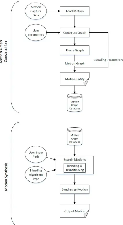
4.1 The overview of the human motion synthesis system. . . 22

4.2 A trivial motion graph. Left: A motion graph built from a data set of two clips. Right: The original clips (edges) are divided into smaller segments and new nodes are inserted. A new edge (transition) can be created by connecting two individual nodes. . 24

4.3 Point clouds of two frames. Left: formed by extracting the neigh-borhood of L = 9 frames after the posture of run motion. Right: formed by extracting the neighborhood of L = 9 frames before the posture of walk motion. . . 25

LIST OF FIGURES x

4.4 2D error matrix of walk motion and run motion. The entry (i, j) is the distance value between frame i of the first motion and frame j of the second motion. Lighter values correspond to smaller dis-tances and the green cells indicate local minima. . . 27 4.5 Transition creation from motion A to motion B. . . 27 4.6 A rough motion graph. The largest strongly connected component

is (1, 2, 3, 5, 6, 7). Node 8 is a dead end and node 4 is a sink. . . 29 4.7 A motion graph constructed from a 24 seconds of motion capture

data (2880 frames at 120fps). . . 30 4.8 Two different graph walk of same motion graph with same start

node motion clip. Yellow line represent the user sketched path, white lines represent the edges in the graph walk and red line represents the actual path followed by the character. Left: Graph walk with 0 motion clip preference error margin which means no preference. Right: Graph walk with 50 motion clip preference error margin. . . 33 4.9 The blend term α which is the equal to the proportion of current

elapsed time to total transition time in linear blending. . . 36 4.10 The blend term α which is the calculated by cubic polynomial

function of t in cubic blending. . . 37 4.11 The blend term α curves for two different Ci values. Left: Ci = 1,

linear curve and Right: Ci = 2, quick anticipation. . . 39

5.1 The effects of motion data size on motion graph construction. . . 41 5.2 The effects of point cloud size on motion graph construction. . . . 42 5.3 The effects of error threshold on motion graph construction. . . . 43

LIST OF FIGURES xi

5.4 Motion synthesis result using linear blending. Yellow line repre-sents user-sketched path and magenta line reprerepre-sents motion path generated by using linear blending. . . 45 5.5 Motion synthesis result using cubic blending. Yellow line

repre-sents user-sketched path and magenta line reprerepre-sents motion path generated by using cubic blending. . . 46 5.6 Motion synthesis result using anticipation-based blending. Yellow

line represents user-sketched path and magenta line represents mo-tion path generated by using anticipamo-tion-based blending. . . 46 5.7 Motion synthesis results. Blue line represents user-sketched path,

green line represents motion path generated by using linear blend-ing, red line represents motion path generated by using cubic blending and cyan line represents motion path generated by us-ing anticipation-based blendus-ing. . . 47 5.8 A running motion with anticipatory behavior to jumping motion

created by (top) cubic blending and (bottom) anticipation-based blending. . . 48 5.9 Motion synthesis result with no motion clip preference. Yellow line

represents user-sketched path and magenta line represents motion path result with no motion clip preference. . . 49 5.10 Motion synthesis result with motion clip preference. Jumping clip

preference error margin is set to 100. Yellow line represents user-sketched path and magenta line represents motion path result with motion clip preference. . . 49 5.11 Motion synthesis results. Blue line represents user-sketched path,

green line represents motion path result with no motion clip pref-erence and motion path result with motion clip prefpref-erence. . . 50

List of Tables

5.1 The system configuration. . . 40 5.2 Sample rate evaluation. . . 44

Chapter 1

Introduction

1.1

Motivation

Character animation especially human animation is an important part of diverse range of media, such as feature films, video games and virtual environments. However, developing an intuitive interface for both professional animators and novice users to easily generate realistic human animation remains one of the great challenges in computer graphics. Creating a realistic human motion is a difficult task. The human body has a complicated structure that can perform motions ranging from subtle actions like breathing to dynamic actions like run-ning. Moreover, people are experts in detecting anomaly in human motions since they have observed human motions throughout their lives.

There are three main approaches for human animation generation. The first approach is keyframing in which an animator specifies important poses of the character at key moments and computer calculates the in-between frames via interpolation techniques. The second approach is to use physical simulation tech-niques to derive the human motions. Although physical techtech-niques can gener-ate physically correct human animation, realism is not guaranteed. In addition, most of the physical techniques are computationally expensive and difficult to

use. Hence, this approach has not been used with much success for realistic hu-man animations. The last approach is to use motion capture, which records the human motions via sensors.

As the sensor technology has improved and the cost of sensors decreased, the interest in using motion capture technology for human animation has increased. The main challenge that the animator face with is to create sufficient details to achieve realism in human motion. Creating details in keyframing approach is extremely labor intensive. However, with motion capture technology, the details are captured and present immediately.

However, the main problem with motion capture is that the recorded motion data is not flexible. It is difficult to modify a captured data after it has been collected. Therefore, the animator has to know what kind of motion he wants in advance. Otherwise, new motion capturing process is needed even for minor changes. In spite of developing technology, motion capture is still a complex and time consuming process for repetitive capture. Therefore, motion synthesis techniques, which make the data reusable by synthesizing new motions, gain im-portance. They enable dynamic synthesis of motion data and interactive control of 3D avatars while preserving the realism of the motion capture data.

1.2

Goal

The objective of this thesis is to synthesize realistic human motion using three different blending types. In addition, the proposed system also enables users to specify motion clip preference. Therefore, users can have more control over result motions, which is not available in standard motion graph.

Our system composed of two main parts. The first part includes the motion graph construction and the calculation of parameters that are needed during the real-time motion synthesis. The user first loads the motion capture data into the system where he can also play the original motion data to ease the motion clip selection. After finalizing the motion dataset, the calculation and the graph

construction are done and the resulting data is saved into standalone database file. The second part synthesizes new motions depending on the blending algorithm and the motion clip preference (if provided). New human motion is synthesized in real-time using any of the database files created before and the user specified path constraint. This separation increases both system reusability and the efficiency.

1.3

Outline

The rest of the thesis is organized as follows. Chapter 2 presents background on skeleton and motion representation. Chapter 3 describes some of the distin-guished works on human motion synthesis. Chapter 4 provides a detailed expla-nation of our work. Chapter 5 shows the results and demonstrate performance and accuracy of the system. Chapter 6 concludes our thesis by summarizing the outcomes and suggesting some ideas for further work.

Chapter 2

Background

2.1

Skeleton Representation

Human models include high number of primitives and deformable parts. Manipu-lation of such complex model by considering each primitive separately is not easy. They should be treated systematically. For example, when an animator wants to transform the leg of the model, he should be able to do it without caring every single primitive that needs to be transformed with leg. This can be achieved by partitioning the model into rigid parts from joints and imposing a hierarchy on these parts. Figure 2.1 shows a skeleton hierarchy of a human leg. It consists of bones femur, fibula and foot connected with the joints knee and ankle. Femur is the highest part in the hierarchy. Each part in the hierarchy lives in the coor-dinate system of its parent. Transformation on femur directly affects the fibula and foot. Therefore, to move the complete leg of the model, it is enough to move the femur.

Figure 2.1: A skeleton hierarchy of a human leg.

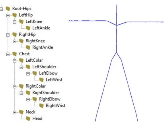
Humanoid Animation standard ISO/IEC FCD 19774 [1], called H-Anim, de-fines a framework for articulated humanoid models. An H-Anim file contains a joint-segment hierarchy. Each joint node may contain other joint nodes and a segment node that describes the body part associated with the joint node. How-ever, in practice joint and segment nodes are merged into one structure, called bones, for simplicity. Hence, bones can be considered as a hierarchy of segments where the connections implicitly specify the joints. Figure 2.2 shows an example representation of hierarchical human skeleton, which is compromised of bones.

Figure 2.2: A hierarchical human skeleton.

2.2

Motion Representation

Hierarchical model enable us to represent different state of complex human model. Each bone except the root bone in the hierarchy has exactly one parent and they specify orientation relative to coordinate system of theirs parent. However, the root bone, which has no parent, specifies orientation and position relative to a fixed coordinate system (world coordinate system). Therefore, if we have humanoid model with n + 1 bones including the root bone, we can define motion M (t) as a multidimensional function as

where pr(t) is position of the root bone and qr(t) is orientation of the root bone

in world coordinate system. Moreover, q1(t), ..., qn(t) are the orientations of

re-maining n bones in hierarchy relative to the coordinate systems of their parents at time t.

Equation (2.1) provides skeleton pose (frame) at any time t. Hence, motion clip for a time interval (ti, tf) can be defined as set of frames M (ti), ..., M (tf) that

Chapter 3

Related Work

Motion synthesis methods can be classified into three major categories: manual synthesis, physically-based synthesis, and data-driven synthesis. The following sections provide detailed explanations of each category together with notable studies.

3.1

Manual Synthesis

Manual synthesis is the oldest motion synthesis technique. This concept goes back to 2D hand-drawn animation. In cartoon animation every single frame need to be drawn by hand. It is time consuming and expensive to have your talented animators drawing all pictures. Therefore using the key frames technique they distribute the work. The talented animators only draw the most important frames called keyframes. Afterwards, less talented animators complete the in-between frames according to keyframes [2].

Similar idea is also used in 3D computer animation. Keyframes, which are the important pose of the character at key moments, are manually specified. These poses are then smoothly interpolated to produce in-between frames by the computer. Burtnyk et al. [3] describes basic interpolation techniques for keyframe

animation. Keyframing gives animators detailed control over the animations. But, interpolating poses rarely produce realistic looking motion. Animators add additional keyframes when interpolation fails to produce realistic looking motion. Therefore, keyframing can be very challenging and time consuming. However, it remains popular for application such as cartoons where the motion does not have to be realistic.

3.2

Physically-based Synthesis

Physically-based techniques try to reduce the animator’s work by using physic laws such as Newton’s laws and conservation of energy to determine the motion. Although physical techniques have successfully been applied for animations such as cloth animation (DeRose [4]), or fluid animation (Foster and Fedkiw [5]), human motion generation via these physical techniques remain challenging.

Physical techniques require information more than joint angles and position as shown in Equation (2.1) to generate a human motion. Information such as mass distribution for each body part and torques generated by each joint also needed. Although average mass distribution information can be obtained from biomechanics literature [6], finding joint torques for particular motion is not easy. Controller-based dynamic approaches use controllers such as proportionalderiva-tive servos to control the joints. Several approaches have been proposed to ease the controller design. Hodgins et al. [7] use finite state machines, Laszlo et al. [8] apply limit cycle control to adjust the joint controllers, and Yin et al. [9] propose a balance control strategy to the controller design.

Controller-based approaches require large number of control parameters. These parameters are usually not intuitive for users. An alternative approach is spacetime constraint and optimal control which is known shortly as space-time constraint. This approach is originally from the field of robotics and it was adapted to computer graphics community by Witkin and Kass [10]. They de-scribe procedural animation of a character inspired by the jumping desk lamp

from Pixar’s short film “Luxo Jr”. This character has only three joints and it has simple angular springs of time-varying qualities at each joint as muscles. In contrast to most previous methods that consider each frame of motion inde-pendently, spacetime constraint considers the entire animation as a numerical problem. Generally, physical parameters of the character such as masses of each limb or spring constants of the joints are specified. Then, using constraint like leg and arm position at specific time or obstacles, an animator can control the char-acter. Finally, motion is determined by solving constraint optimization problem where the energy is minimized while satisfying the constraint.

Spacetime constraint approaches are popular due to their optimal energy so-lution and intuitive user control. However, for human characters, the system is very hard to solve because it is very high dimensional and non-linear. A number of methods have been proposed to reduce the optimization space while preserving the personality of motion. Popovic and Witkin [11] simplify the complex human character to reduce the degrees of freedom (DOF) that are essential for particular motion. Safonova et al. [12] compute the low dimensional space using Principal Components Analysis (PCA) and apply physical constraint optimization on low dimensional space.

Physically-based motion synthesis can automatically generate physically cor-rect human motions. However, physical correctness does not guarantee that the motion looks natural, because certain aspects of human motion such as styles, emotions and intentions cannot be governed by physic laws. Moreover, most physically-based motion synthesis techniques are computationally expen-sive. Generating a few seconds long motion usually takes several minutes.

3.3

Motion Capture

The main problem of physically-based motion synthesis is that the generated motion does not look natural. Instead of creating motion in computer, the real

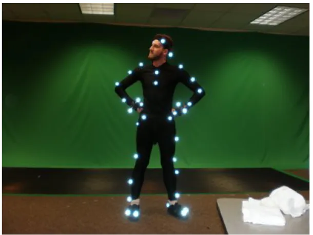
movement of human can be recorded using motion capture technologies. Fig-ure 3.1 shows an actor in motion captFig-ure process.

Figure 3.1: An actor performing in a motion capture process.

Motion capture devices record live motions of an actor by tracking number of key points over time. The recorded motion data is then converted into more usable form by post processing steps. The recorded raw motion is re-targeted into a standard skeleton with bone hierarchy and saved on files, after its noise cleaned. The resulting motion capture data saved in files is of the form

M (t) = (pr(t), qr(t), q1(t), ..., qn(t)), (3.1)

3.4

Motion Capture File Formats

The success of motion capture technique has led to a number of companies that can record and provide motion data. However, many of these companies has developed their own file formats. Some of these formats are Acclaim ASF/AMC, Biovision BVA/BVH, BRD, CSM and C3D. Although there is no standard motion capture file format, the most commonly used format in computer animation are Acclaim ASF/AMC and Biovision BVA/BVH. Brief information about these file formats are given in the following sections.

3.4.1

Biovision BVH File Format

The Biovision Hierarchical Data (BVH) file format was developed by motion cap-ture company called BioVision. The BVA format is also developed by BioVision company and it was the precursor to BVH format. The BVA format is an ASCII file that contains no skeleton hierarchy but only the motion data. However, BVH format is a binary file containing both skeleton and motion capture data.

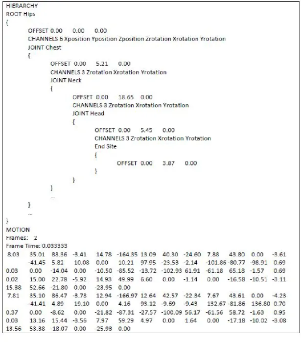
The BVH format has two sections: the hierarchy section and the motion section. The hierarchy section contains the skeleton hierarchy of a human body, as well as the local translation offsets of the root and the joints. The motion section contains the root’s global translation and rotation values, and the joints’ local rotation values relative to their parents. Figure 3.2 shows an example BVH file.

The BVH format is very flexible and relatively easy to edit. However, it lacks a full definition of the initial pose. Another problem with BVH format is that the BVH format is often implemented differently in different applications. One BVH format that works well in one application may not be interpreted in another.

Figure 3.2: An example of BVH file.

3.4.2

Acclaim ASF/AMC File Format

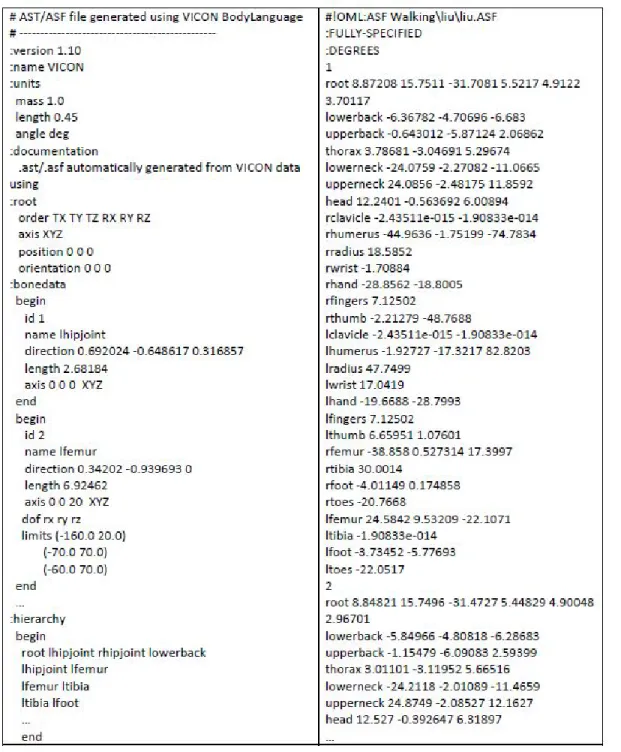
Acclaim Skeleton File (ASF) and Acclaim Motion Capture (AMC) are the file formats for storing motion capture data developed by Acclaim Entertainment, Inc. The format has two separate ASCII-coded files: ASF and AMC. The reason

to separate skeleton file from motion file is to have a single skeleton file for each actor. Therefore, a skeleton file of an actor can be used with multiple different motion files recorded by that actor. Figure 3.3 shows an example of both ASF and AMC files.

The ASF file contains all the information of the skeleton, such as its units, bones, documentation, root bone information, bone definitions, degrees of free-dom, limits, hierarchy definition, and file names of skin geometries. However, it does not have the motion data itself. In addition, the ASF file contains an initial pose for the skeleton.

The AMC file contains the actual motion data for the skeleton defined by an ASF file. The bone data is sequenced in the order which is specified as the order of transformation in the ASF file.

In our implementation, Acclaim ASF/AMC format is used. It is simple and human readable format which is very important to verify the animation results. Moreover, many publicly available motion capture databases, such as Carnegie-Mellon University (CMU) database [13], support this format.

3.5

Data-driven Synthesis

The idea of motion capturing originates from the field of gait analysis, where locomotion patterns of humans and animals were investigated. In the past, such motion capture data was difficult to obtain due to cost of sensor devices. However, with technological progress, motion capture data or simply mocap data became more available. Therefore, the interest in using motion capture for creating char-acter animation is increasing. Motion capture gains popularity in film and video game industry because realism of animation is guaranteed.

On the other hand, motion capture technique still has problems despite of technological progress. The main problem is the lack of flexibility. It is diffi-cult to modify a captured motion data after it has been collected. Therefore, an animator should know what exactly he wants. However, it is not easy to decide whole motion because creating a character animation is an evolutionary process. Usually, an animator has only coarse impression of the desired motion before he captures. Minor correction could always be needed anytime thereafter. In addition, same motion captured data cannot be used even for very similar animations. A new motion captured data, which is specific to the animation, is required. These problems prevent the reuse of motion captured data which turns the motion capture into costly and labor intensive task. As a result, many researchers have focused on problem of editing and synthesizing motion captured data once it is collected.

3.5.1

Signal-based Animations

In these methods, motion data is treated as a set of signals. Thus, signal process-ing techniques such as multiresolution filterprocess-ing and spectral analysis are applied to these signals to quickly modify captured motion data. However, manual adjust-ment of the filtering and spectral analysis methods parameters and good artistic skills are still required to obtain desired motion.

motion data to extract characteristic function of an emotional motion. This char-acteristic function can then be applied to different motion to exhibit the same emotional characteristic. Similarly, Amaya et al. [15] extract emotional trans-forms of motion captured data but without using Fourier transform. Bruderlin and Williams [16] show that by representing motion data as signals, filtering methods and other common signal processing methods such as multiresolution filtering, waveshaping, timewarping and interpolation can be applied to modify motion characteristics.

3.5.2

Move Trees

The video game industry relies on manually created graph structures, called move trees [17], to represent transitions that connect several motion clips. They are commonly used in video games to generate realistic human motion. Each node in move trees represents a unique motion clip, and the edges between these nodes represent transitions between clips. To construct a move tree, game developers first design a finite state machine to represent all the behaviors required by the game and all logically allowed transitions between behaviors. They capture the motions according to this pre-planned finite state machine so that initial motions have similar start and end pose for looping. Then, they manually edit the cap-tured motion clips and choose the best place in the motions for good transitions according to the finite state machine.

Although move trees are well suited for highly interactive animations, the creating process is labor intensive. Motion clips, structure of move trees, and game logic should be carefully planned before development and then created manually. This manual effort makes large move trees expensive and fragile. In addition, adding, removing or changing a motion clip is almost impossible without reconsidering the whole process over again.

3.5.3

Motion Graphs

Inspired by the technique of Schodl et al. [18], which allows a long video to be synthesized from a short clip, several researchers have investigated the possibility of automatically constructing a directed graph structure like move trees and au-tomatically searching them to find the appropriate motion sequence [19, 20, 21]. This fully automatic approach is termed as Motion Graphs and unlike move trees; it does not require any manual effort at all.

Motion Graphs were introduced by Kovar et al. [21]. They provide an au-tomatic method to create continuous streams of character motion in real-time. Motion graph embed multiple motion captured data into directed graph structure where graph nodes represent the motion captured frames and graph edges repre-sent possible transitions between the motion frames. Then continuous streams of character motion can be produced by simply walking the graph and playing the motion captured frames encountered along each edge.

Motion graphs have emerged as a very promising technique for automatic human motion synthesis both for interactive control applications [20, 22] and also for offline sketch-based motion synthesis [19, 21, 23, 22]. Although this thesis work focus on offline sketch-based motion synthesis, it can also be adjusted to interactive control applications easily without modifying any motion synthesis algorithms.

Arikan et al. [19] present a similar graph structure with motion constraint. They automatically construct a hierarchical graph from a motion database and then used a randomized search algorithm on the constructed graph to extract appropriate motion that satisfies user constraints. Lee et al. [20] also construct a similar graph and generate motion via three user interfaces: choice, sketch and performance (vision-based) interface. In the choice interface, the user is continuously presented with a set of possible animations that can be played from the current pose. In the sketch interface, the user sketches the 2D path and the database is searched to find a motion sequence that follows user path. In the performance interface, the user records desired motion in front of the camera.

Then visual features of the recorded video is extracted and queried in motion graphs. The closest motion to the recorded video is identified and selected from motion database. However, the performance interface suffers from occlusion. Moreover, it has three seconds delay.

3.5.4

Motion Blending

Motion blending, which allows the generation of new motions by interpolation, is an integral part of many motion synthesis researches. Motion blending techniques are also used to produce smooth transitions between two different motions.

Perlin’s real-time procedural animation system [24] is one of the earliest works on motion blending. In this system, blending operations are applied on a user selected dataset to create new motion and transitions between these motions via interpolations. Guo and Roberge [25] and Wiley and Hahn [26] used linear interpolation and spherical linear interpolation on a set of hand selected example motions to synthesize new motions. For example, Wiley and Hahn interpolated among a set of reaching and pointing motions to be able to point new directions. Rose et al. [27] implemented a system that use radial basis functions (RBFs) to interpolate motions located in an irregular parametric space. They defined analogous structures for simplicity; the base example motions are called as verbs and the control parameters that describe these motions, such as mood, are called as adverbs. As a result of their work, Rose and his colleagues were able to gener-ate new motions by interpolating example motions with new values for adverbs. These motions included a set of walks and runs of varying speed and emotions.

Shum and his colleagues [28] proposed a method to synthesize preparation behavior for the next motion to be performed. Their research shows that this kind of preparation behavior results in more natural motion sequences compared to traditional linear interpolation technique [29].

Safonova and Hodgins [30] analyzed interpolated human motions for physical correctness. They evaluated interpolated motions in terms of some basic physical

parameters: (1) linear and angular momentum; (2) foot contact, static balance and friction on the ground; (3) continuity of position and velocity between phases. Their results show that, in many cases interpolated motions satisfy the physical properties.

Linear interpolation for position values and spherical linear interpolation for joint orientations are widely used for creating transitions between motions [24, 27, 31]. In this thesis work, we analyzed three different motion blending algorithms. The first one is linear interpolation algorithm which is also used in standard motion graphs. Second one is cubic interpolation algorithm and the last one is anticipation-based interpolation algorithm.

Chapter 4

Human Motion Synthesis

In this thesis work, we present a real-time motion synthesis system that follows user path. Figure 4.1 shows the general overview of our system. The system composed of two main stages.

The first stage is motion graph construction stage. In this stage, the user first provides the motion capture data in Acclaim ASF/AMC File Format. An ASF skeleton file and set of AMC motion data files are loaded via graphical user interface and system converts loaded files to its internal structure. Then, the user can either play the original motion or construct motion graph with set of input parameters. This stage is an off-line stage. However, it only needs to be done once. After constructing the graph, system saved it to database so that it can be used anytime in second stage. Blending and transitioning parameters that are needed in the second stage are also calculated in this off-line stage and saved to database with the motion graph.

The second stage is the motion synthesis stage. This stage synthesizes mo-tion in real time using the data from the first stage. In this stage, the user sketches the desired motion path. Then, the output motion following the desired path is generated by traversing the motion graph. The transitioning between similar motions in the graph is done by blending. The user can select the blend-ing algorithm type among three different algorithms that are linear, cubic and anticipation-based. Computationally costly processes, such as graph construction and the parameters calculations, are performed in the off-line stage. Therefore, the motion generation, which is the second stage, can be done in real-time. This separation in the system flow increases the efficiency of the system. Users can synthesis new motions without doing the first stage again.

4.1

Graph Construction

As explained in Chapter 3, creating human animation from scratch is difficult. Manual synthesis techniques are both time consuming and fail to produce realistic human motion. Physically-based techniques can generate a physically correct human motion. However, the generated motion does not look natural. Therefore, we adopt data driven approach.

Motion capture systems record human motion from a live actor. A motion clip is composed of a sequence of poses which are sampled at a fixed frame rate. Therefore, a motion clip can contain only a limited number of captured behaviors for a finite duration. However, a collection of motion clips presents an opportunity to synthesize longer motions by transitioning similar poses from different motion clips. Motion graphs automatically produce new sequences of motions of arbitrary length from a finite set of input motion.

Motion graph is a directed graph where edges are the motion clips and nodes are the choice points connecting these edges. Each edge contains either original motion data or automatically created transition. A trivial motion graph can be constructed by placing all these motion clips as edges. Then there are two nodes

for each edge, one node for the beginning and one node for the end of each edge. Figure 4.2 shows an example of trivial motion graph. New nodes can be inserted to graph by dividing the edges (original clips) into smaller segments. Then, new edges (transitions) can be created to connect these nodes and to increase the graph connectivity. More interesting graph requires better graph connectivity.

Figure 4.2: A trivial motion graph. Left: A motion graph built from a data set of two clips. Right: The original clips (edges) are divided into smaller segments and new nodes are inserted. A new edge (transition) can be created by connecting two individual nodes.

Two original motion data cannot be sufficiently similar to connect directly. Therefore, a transition edge is needed which is created by blending the original motions. Creating a transition is an important, yet difficult animation problem. Linear blending is the commonly used technique to create smooth transitions. The rest of this section explains our solution including distance metric for motions and transition creation with different blending algorithm.

4.1.1

Distance Metric

Creating transition is as hard as creating human motion from scratch. Transi-tions between different moTransi-tions such as run and crawl requires several seconds of anticipation motion even for humans in real life. However, smooth transition can be created between similar poses with blending techniques. Therefore, we need a distance metric to find similar frames in motion data. The Distance function is

D(Ai, Bj) where Ai is the ith frame of the motion A and Bj is the jth frames of

motion B. The smaller the value is, the more similar the frames are.

The motion data are composed of positional and rotational vector data of root and joints as shown in Equation (2.1). Therefore, a naive distance function could be the sum of the Euclidean distance of the corresponding root and joints of two frames. However, a good distance function should consider not only the static posture difference but also dynamic motion difference. For example, two standing poses might be similar if we consider only static posture difference. However, one might move the right foot while other might move the left foot.

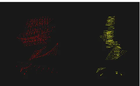
We adopt to use point cloud metric method proposed by Kovar and his col-leagues [21]. This technique takes into account both static posture difference and dynamic motion difference. In this method, each root and the joint of the skele-ton is treated as a point. Therefore, one frame forms a point cloud. However, to address the dynamic motion difference between Ai and Bj, we consider two

point clouds of length L frames. The first point cloud is formed by extracting the neighborhood of L frames after Ai and the other one is formed by extracting

L frames before Bj. Figure 4.3 shows a point cloud of two frames.

Figure 4.3: Point clouds of two frames. Left: formed by extracting the neigh-borhood of L = 9 frames after the posture of run motion. Right: formed by extracting the neighborhood of L = 9 frames before the posture of walk motion.

The distance function is defined as the sum of all squared Euclidean distances between corresponding points, minimized over all translations in the floor plane and rotation about the vertical axis:

D(Ai, Bj) = min θ,x0,z0 n X k=1 wkkpk− Tθ,x0,z0p 0 kk 2 , (4.1) where pk and p0k denote the kth point in the point clouds for Ai and Bj,

respec-tively, and Tθ,x0,z0 is a rigid transformation composed of a rotation about the y

(vertical) axis of θ degrees and a translation of (x0, z0) on the floor plane. The

scalar wk is the multiplication of the joint weight, telling how important the joint

and the frame weight to reduce importance towards the edges of the window. In order to calculate the Euclidean distance, two points needs to be in the same coordinate system. Therefore, we first apply align transformation Tθ,x0,z0

to the points p0_k in the point clouds of Bj so that pk and p0k are in the same

coordinate system. The align transformation has the following solution:

θ = arctan P iwi(xizi0− x 0 izi) −P1 iwi (¯x ¯z0_{− ¯x}0_z)¯ P iwi(xix0i+ ziz0i) −P1 iwi (¯x ¯x0_{+ ¯z ¯z}0₎, (4.2) x0 = 1 P iwi (¯x − ¯x0_{cos θ − ¯z}0_{sin θ), (4.3)} z0 = 1 P iwi (¯z + ¯x0_{sin θ − ¯z}0_{cos θ), (4.4)} where ¯x =P

iwixi, ¯z =Piwizi and the other barred terms are defined similarly.

In order to find the right transformation matrix, we take into account all points in the point cloud.

4.1.2

Transition Creation

The distance between every pair of frames is calculated with the distance function in Equation (4.1), which results in a 2D error matrix. Figure 4.4 shows an example

2D error matrix. Then we find all the local minima on the 2D error matrix by comparing the value of each point with its eight neighbors. These local minima form our candidate transition points.

Figure 4.4: 2D error matrix of walk motion and run motion. The entry (i, j) is the distance value between frame i of the first motion and frame j of the second motion. Lighter values correspond to smaller distances and the green cells indicate local minima.

Although a local minimum implies a transition better than its neighbors, it does not have to be a good transition. Its error value still could be high. However, we are interested in local minima with small error values. Therefore, we need a threshold value to extract the good transition points among candidate ones.

If D(Ai, Bj) is the one of the local minimum and also meets the threshold

requirements, then a transition from Ai to Bj can be created by blending the

frames. We blend the frames Ai to Ai+L−1 with frames Bj−L+1 to Bj. Figure 4.5

shows an example transition creation between motion A and B.

In order to blend motions, we need to apply the appropriate 2D align trans-formation to motion B so that both motions are in the same coordinate system. The transformation solution is provided in Equations (4.2) to (4.4). Then, on frame k of the transition (0 ≤ k < L), we interpolate the root position and the joint rotations: pk = (1 − α) × pAi+k + α × pBj−L+1+k, (4.5) q_ki = Slerp(α, q_Ai i+k, q i Bj−L+1+k), (4.6)

where pk is the root position on the kth transition frame and qki is the rotation

of the ith joint on the kth transition frame. The calculation of the blend term α will be explained in Section 4.2.

4.1.3

Graph Pruning

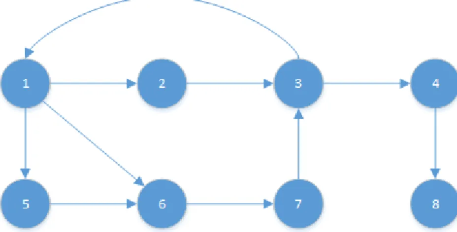
The constructed motion graph in Section 4.1.2 cannot be directly used for motion search. It may contain dead end nodes, which are nodes that are not part of any cycle in the graph. The motion graph cannot synthesize motion indefinitely if such a node is entered. In addition, the graph may also contain other nodes, called sinks. Although sinks may be a part of one or more cycles , they can only reach part of the total numbers of nodes in the graph. These two kinds of nodes may cause the motion search to be halted. Figure 4.6 shows an example rough motion graph which contains dead end and sink nodes.

Figure 4.6: A rough motion graph. The largest strongly connected component is (1, 2, 3, 5, 6, 7). Node 8 is a dead end and node 4 is a sink.

These nodes may halt the motion search. Hence, we prune the graph to eliminate these problematic nodes such that it is possible to generate arbitrary long stream of motion using as much of the motion data as possible. We calculate the largest strongly connected component (SCC) of the graph which is a maximal set of nodes such that every node can reach to all other nodes in the graph. The SCCs can be computed in linear time using Tarjan’s algorithm [32]. Any edge that does not connect two nodes in the largest SCC is discarded. Similarly, nodes without any edge are eliminated from the graph.

4.2

Motion Synthesis

In Section 4.1, we have created motion graph with its blending parameters and saved it to database. In this section, given any motion graph, we will synthesize motions via graph walking. During the graph walk, we blend these motions and create transitions on run time according to the blend parameters calculated and the blend term α.

by applying appropriate 2D align transformation to each edges and concatenat-ing them. However, motion graphs generally have a complicated structure (see Figure 4.7). Users cannot work with the generated graph directly. A naive ap-proach is to build a random graph walks by concatenating the edges one after another. However, this approach generates completely random motions since we do not have any control over the generated motion. Another approach is to apply shortest path graph algorithm [33]. This approach allows users to build motions that connect two given edges. However, there is still no control over the gener-ated motion. We cannot specify the character direction and the end point of the motion. Therefore, we need a technique to extract an optimal graph walk that conforms to user’s specifications from the motion graph.

Figure 4.7: A motion graph constructed from a 24 seconds of motion capture data (2880 frames at 120fps).

We cast the motion synthesis as a search problem and use branch and bounds to increase the search efficiency. The rest of this section describes search al-gorithm, optimization criteria for graph walk, calculation of the blend term α depending on three different blending algorithms and conversion of graph walk to a displayable motion.

4.2.1

Motion Search Algorithm

The user supplies an optimization criteria Ocf (w , e), which is explained in Sec-tion 4.2.2, to evaluate the error accumulated by appending an edge e to existing graph walk w. The total error Erf (w ) of a graph walk is:

Erf (w ) = Erf ([e1, e2, ..., en]) = n

X

i =1

Ocf ([e1, e2, ..., ei −1], ei), (4.7)

where e1, e2, ..., en−1 is the existing edges when appending the edge en. We

as-sumed that Ocf (w , e) is never negative. Therefore, the total error cannot decrease by adding an edge to a graph walk.

The start node of the walk can be randomly chosen by the search algorithm. However, the user must provide a halting condition of the graph walk. A graph satisfying a halting condition is said to be complete so no more edges can be added.

A simple way of optimizing the error function Erf is to generate all complete graph walks with depth-first search algorithm and selecting the minimum one. However, generating all the complete graph walks has performance issue. Hence, we use branch and bound algorithm in which we prune any graph incapable of producing an optimal graph walk, to increase the efficiency. We further increase the efficiency by exploiting the fact that Erf (w ) can never decrease by adding edges. During searching process, the algorithm keeps track of the optimal com-plete graph walk wopt and halts the branch of the search unless the current error

Although branch and bound algorithm reduces the graph walks via pruning the incapable branches, the number of graph walks searched still grows exponen-tial. This problem might prevents real time motion synthesis. Search process takes large amount of time, especially when we generate long stream of motion. Therefore, we generate a graph walk incrementally and restrict the search time. At each step, we search for an optimal graph walk of s frames. Then, only the first r frames of this graph walk is retained and the last retained node is chosen as start node of next search step. In our implementation, we search for frames which is at most two seconds away (s ≈ 240 frames) from the start node and retain the frames which is at most one second away (r ≈ 120 frames) from the start node.

In some circumstances the user want to control the motion he synthesized. To achieve this, we let the user to specify preference error margin for each motion clips. The more the preference error margin, the more likely to stay in that motion clip. Moreover, instead of starting a graph walk randomly, we restrict this random choice. The start node has to be random node from the motion that has maximum preference error margin. During branch and bound algorithm, we give priority to motion clip which is equal to the start node motion clip within specified preference error margin. Therefore, in order to change motion clip Erf (wdif) should be less than Erf (wcurrent) − Pem(mc) where wdif is a graph

walk of different motion clip from the start node motion clip, wcurrent is the graph

walk from the same motion clip and Pem(mc) is the preference error margin of motion clip mc. However, as the preference error margin increase, the quality of graph walk decreases (see Figure 4.8).

Figure 4.8: Two different graph walk of same motion graph with same start node motion clip. Yellow line represent the user sketched path, white lines represent the edges in the graph walk and red line represents the actual path followed by the character. Left: Graph walk with 0 motion clip preference error margin which means no preference. Right: Graph walk with 50 motion clip preference error margin.

4.2.2

Optimization Criteria for Path Synthesis

An optimization criteria function Ocf (w , e) and a halting condition is needed to extract motion from the constructed motion graph. In order to get these information from the user, we apply path synthesis that is generating a motion stream that follows a user specified path. We collect the path data P (pti, li) from

the user sketch path where pti is the ith point on the path and li is the arc length

from start point to pti.

path P , we evaluate the deviation between P0 and P . We first project the charac-ter’s root position pt0 onto the ground at each frame and compute the arc length l0_e,i from the start of path P0 to pt0_e,i that is the root position at ith frame on edge e. Then, we find the point pt on path P whose arc length l is the same with l0_e,i. The point pt is computed by linearly interpolating pti−1 and pti with the factor

β, which is calculated as β = l 0 e,i− li−1 li− li−1 . (4.8)

The cost of appending edge e to graph walk w, Ocf (w , e), is then calculated by the sum of squared distance between pt and pt0_e,i for all n frames on edge e.

Ocf (w , e) =

n

X

i=1

kP0(pt0_e,i, l0_e,i) − P (pt, l0_e,i)k2. (4.9)

We should first apply 2D align transformation to edge e to make sure that they are in the same coordinate system when calculating p0_e,i.

The halting condition of the motion extraction is that the total arc length of path P0 exceeds the total arc length of path P . Moreover, if an arc length of a frame exceeds the total length of path P , the corresponding point is mapped to the last point on path P .

In case the character is at exactly the correct point of P , it can infinitely accumulate zero error by staying there. Therefore, we use a small amount of forward progress gamma on each frame to avoid staying infinitely. l_e,i0 in Equa-tion (4.9) becomes max(l_e,i0 , l0_e,i−1 + γ). In our implementation, we set forward progress γ = ₁₅2.

4.2.3

Conversion of Graph Walk into Motion

Once we extract the optimal graph walk, we need to convert it into continuous motion stream. Graph walk is composed of edges which are actually piece of

motion. Therefore, we can generate motion stream by placing these edges of graph walk one after another in the same order. There are two important issues we need to pay attention. The first one is to place the edges of the graph walk to correct position and orientation. Therefore, we need to apply correct 2D align transformation to each transition so that the frames are aligned in the same coordinate system (Section 4.1.1). The second issue is blending of the transitions. We need to calculate the blend term α so that we can convert the transition into motion using Equations (4.5) and (4.6). The calculation of the blend term α according to three different blending algorithms is explained in the following section.

4.2.4

Blend Algorithms

Transitions are crucial part of motion graphs. They have direct effects on the generated motion quality. We generate transitions using three different blending algorithms. The First one is linear blending which is used in standard motion graph. The second one is cubic blending and the third one is anticipation-based blending.

All the parameters needed to generate transition motion is calculated and saved during motion graph construction (Section 4.1). Therefore, in motion syn-thesis part, the user can select any of these blending algorithms and generate motion stream.

Root position of the transition is calculated as:

p = (1 − α) × p`1 + α × p`2, (4.10)

where p`1 and p`2 are the root positions in the locomotions `1 and `2.

The blended joint angles of the ith joint are calculated as:

qi = Slerp(αi, qi_{`1</sub>, q<sub>`}i₂), (4.11) where qi

`1 and q

i

calculation of the blend term α, which is given in the following sections, depends on the user selection blending type.

4.2.4.1 Linear Blending

In linear blending, the blend term α is exactly linear with the time elapsed during transition.

α = tcurrent/ttransition, (4.12)

where tcurrent is the elapsed time during transition and ttransition is the total time

of the transition.

In linear blending, motion changes linearly from locomotion `1 to `2 as time

passes (see Figure 4.9). Although this blending can generate plausible motion stream, it lacks naturalism for transition which is especially between different type of motion such as from walking motion to crawling motion. There is no anticipatory behavior in this blending.

Figure 4.9: The blend term α which is the equal to the proportion of current elapsed time to total transition time in linear blending.

4.2.4.2 Cubic Blending

In cubic blending, the blend term α is calculated by a cubic polynomial function:

α = 2 × t3− 3 × t2_{+ 1, (4.13)}

where t = tcurrent/ttransition. The parameter tcurrent represents the elapsed time

during transition and ttransition represents the total transition time.

Motion does not changes linearly from locomotion `1 to `2 (see Figure 4.10).

There is an anticipation for the locomotion `2 at the beginning and at the end of

the transition. However, the middle of the transition is almost linear. Although this blending can generate some anticipatory behavior between two motions, the user cannot specify different anticipation parameters for different body parts of the character. Hence, all the body parts of the character has the same anticipatory behavior.

Figure 4.10: The blend term α which is the calculated by cubic polynomial function of t in cubic blending.

4.2.4.3 Anticipation-based Blending

In anticipation-based blending, the blend term α is calculated as:

α = Ciq_{1 − (1 − t)}Ci, (4.14)

where Ci is a constant which can be set individually for each joint and t =

tcurrent/ttransition. The parameter tcurrent represents the elapsed time during

tran-sition and ttransition represents the total transition time.

Using the constant Ci, the user can specify different behaviors for each joints.

Hence, we can generate transition which needs different anticipatory behavior for different joints such as transition from walking to boxing (see Figure 4.11). The arms of the humans generally switch to boxing style quickly while the lower body part adapted to boxing linearly.

Figure 4.11: The blend term α curves for two different Ci values. Left: Ci = 1,

Chapter 5

Evaluation

In order to test our system, we have conducted a number of experiments on different parts of the system. First, we give brief information about our test platform. Then, we give detailed information about performance and accuracy of the system.

5.1

Experimental Results

In our experiments, we used several types of motion capture data, such as walk-ing, running and jumpwalk-ing, from the motion capture database of Carnegie Mellon University [13]. All the experiments presented in this thesis are performed on a PC with the configuration as summarized in Table 5.1.

Processor 2.50 GHz Intel Core 2 Duo

RAM 3 GB

Graphics Card ATI Mobility Radeon HD 2600 Operating System Windows 7 Professional

5.1.1

Graph Construction

In order to synthesize motion, users have to construct a motion graph. Therefore, we first evaluate the performance of motion graph construction.

As the size of the motion captured data increase, the size of the constructed motion graph increase. Therefore, as seen in Figure 5.1, motion graph con-struction time increases with the number of frames in the motion captured data provided to system.

Figure 5.1: The effects of motion data size on motion graph construction.

Point cloud size also affects the graph construction time. As the point cloud size increases, the number of comparison points in Equation (4.1) increases. Hence, the construction time of the motion graph increases (see Figure 5.2).

Figure 5.2: The effects of point cloud size on motion graph construction.

Error threshold value affects the motion graph construction. As the error threshold value increases, the number of candidate transition and the graph connectivity increases. Therefore, graph construction time increase with simi-lar manner because connectivity increase the post-processing of the graph such as subdividing and pruning (see Figure 5.3).

Figure 5.3: The effects of error threshold on motion graph construction.

In addition, sampling rates also affects the graph construction. Table 5.2 compares four rates (120, 60, 30, 20). For four motions: “walk straight” (416 frames), “turn left” (518 frames), “turn right” (410 frames), “run straight” (135 frames). As we can see, higher sample frequency spends more time in graph construction because higher sample frequency causes more pairs of frames to be involved in graph construction process. Moreover, higher sample frequency means more nodes and transitions in the constructed motion graphs. Therefore, higher sample frequency results in better connectivity in the constructed motion graph.

Sample Rate Graph Number of Number of (frames/seconds) construction transition candidate nodes in

time (seconds) constructed graph

120 71 572 628

60 18 484 431

30 9 402 274

20 7 334 204

Table 5.2: Sample rate evaluation.

Motion graph construction takes significant time and this construction time increase with motion data size, error threshold value and point cloud size. How-ever, graph construction time does not affects the motion synthesis part. We save the constructed graph with its parameters to mog file which is a sqlite motion graph database file. Therefore, we can load motion graph anytime using mog file and synthesize motion in real time.

5.1.2

Motion Synthesis

We generate motions using mog database file which is constructed in Section 4.1 and path synthesis. The user imposes path specifications on motions by sketching a path.

The generated motion is supposed to be as close to the sketched path as possible. Ideal generated motion follows the sketched path perfectly. However, in most cases the path traveled by the character cannot perfectly follows the sketched path because there is not enough original motion data in the motion graph to generate appropriate motions. Our system tries to find an optimal graph walk that fits the specifications using three different blending techniques.

In this section, we test accuracy of these three different blending techniques namely linear blending, cubic blending and anticipation-based blending. Fig-ure 4.9 shows motion synthesis result by using linear blending, FigFig-ure 4.10 shows

motion synthesis result by using cubic blending and Figure 4.11 shows motion synthesis result by using anticipation-based blending. Motion synthesis result generated by linear blending is less accurate than the motion synthesis result generated by cubic blending. However, motion synthesis result generated by anticipation-based blending is as accurate as the one generated by cubic blending (see Figure 5.7).

Figure 5.4: Motion synthesis result using linear blending. Yellow line represents user-sketched path and magenta line represents motion path generated by using linear blending.

Figure 5.5: Motion synthesis result using cubic blending. Yellow line represents user-sketched path and magenta line represents motion path generated by using cubic blending.

Figure 5.6: Motion synthesis result using anticipation-based blending. Yellow line represents user-sketched path and magenta line represents motion path generated by using anticipation-based blending.

Figure 5.7: Motion synthesis results. Blue line represents user-sketched path, green line represents motion path generated by using linear blending, red line represents motion path generated by using cubic blending and cyan line represents motion path generated by using anticipation-based blending.

An example of anticipatory behavior using cubic blending is shown in Fig-ure 5.8 (top). Notice that both the upper body and the lower body have the same anticipatory behavior which makes the second posture unnatural. On the other hand, with anticipation-based blending, the upper body switches to the jumping style quickly comparing to the lower body which has a longer transition period (see Figure 5.8 (bottom)). Hence, a better anticipatory behavior is created by anticipation-based blending. In Equation (4.14), we set Ci = 1.0 for the lower

Figure 5.8: A running motion with anticipatory behavior to jumping motion created by (top) cubic blending and (bottom) anticipation-based blending.

In addition to blending techniques, we let the user to specify motion prefer-ences. For each motion clip, the user defines a preference error margin and we apply these error margins to motion search algorithms. Figure 5.9 shows motion synthesis result with no motion clip preference and Figure 5.10 shows motion synthesis result with motion clip preference. Motion synthesis result with mo-tion clip preference is less accurate because we restrict the graph walk to specific motion clip within error margin (see Figure 5.11).

Figure 5.9: Motion synthesis result with no motion clip preference. Yellow line represents user-sketched path and magenta line represents motion path result with no motion clip preference.

Figure 5.10: Motion synthesis result with motion clip preference. Jumping clip preference error margin is set to 100. Yellow line represents user-sketched path and magenta line represents motion path result with motion clip preference.

Figure 5.11: Motion synthesis results. Blue line represents user-sketched path, green line represents motion path result with no motion clip preference and mo-tion path result with momo-tion clip preference.

Chapter 6

Conclusion

In this thesis, we propose a system that generates a realistic, continuous human motions automatically. This system composed of two stages: online and offline stages. This kind of separation increase the efficiency and usability of the system by reducing the respective processes. The offline stage includes motion graph construction and calculation of required parameters such as blending parame-ters. These results are saved on database file (mog file). Then, the online stage searches the graph and synthesizes new motions that satisfy user requirements using mog file created in the offline stage. Therefore, the second stage (online stage) synthesize new motions in real time depending on blending algorithm type user selects.

The result motions are highly realistic and continuous. They are composed of real human motion captured data and can make a smooth transition to any other motion provided that there are similar poses between the two transferred motions. Results motion can follow the paths specified by users as much as possible. More-over, the user can also specify preference error margin in order to give priority to motion clips during graph walk search. Therefore, the user can control the mo-tion clip types in the generated momo-tion via introducing an error margin. However, without appropriate post processing, the generated motions might presents arti-facts caused by blending of frames. One particularly distracting artifact is that the character’s feet move when they should remain planted, a condition known as

footskate [34]. In future work, we will try to use constraints annotations defining which frames contain a foot-plant and how long this constraint lasts for. Then, the fixed foot positions on the ground are used in post-processing to compute other joints and root positions with an inverse kinematics (IK) solver. Another idea that uses inverse kinematics constraints during interpolation process can also be considered to eliminate an extra post-processing step.

Computation time of the graph walk search is the bottleneck of our system that affects the result motions quality. In spite of branch and bound algorithm, we restrict the search time in order to have a real time motion synthesis system. However, this restriction can generates poor motion paths because of inadequate search time. This situation especially occurs for combination of low sample rates and low transition lengths motion graph parameters which increase search time of the graph. Therefore, an improved search algorithm can generate better motion paths.

Finally, the graph structure is highly controllable, in principle. Therefore, in addition to path synthesis, we can generate motions that satisfy new requirements of the users.

Bibliography

[1] Web3D Consortium and others, “Information technology–computer graph-ics and image processing–humanoid animation (h-anim), iso/iec fcd 19774: 200x.” http://h-anim.org/Specifications/H-Anim200x/ISO_IEC_FCD_ 19774, 2004.

[2] F. Thomas, O. Johnston, and W. Rawls, Disney animation: The illusion of life, vol. 4. Abbeville Press New York, 1981.

[3] N. Burtnyk and M. Wein, “Interactive skeleton techniques for enhancing motion dynamics in key frame animation,” Commun. ACM, vol. 19, pp. 564– 569, Oct. 1976.

[4] T. DeRose, M. Kass, and T. Truong, “Subdivision surfaces in character ani-mation,” in Proceedings of the 25th Annual Conference on Computer Graph-ics and Interactive Techniques, SIGGRAPH ’98, (New York, NY, USA), pp. 85–94, ACM, 1998.

[5] N. Foster and R. Fedkiw, “Practical animation of liquids,” in Proceedings of the 28th Annual Conference on Computer Graphics and Interactive Tech-niques, SIGGRAPH ’01, (New York, NY, USA), pp. 23–30, ACM, 2001. [6] D. A. Winter, Biomechanics and motor control of human movement. John