Development of a Supervisory Controller
for Residential Energy Management Problems
Emre Akg¨un and Melih C
¸ akmakcı
Abstract— In recent years, the infrastructure that supplies energy to residential areas has started to evolve into a multi-source system, just like in automotive industry in which hy-brid electric vehicles (HEVs) have been replacing conventional gasoline vehicles. Multi energy source systems considered as a potential solution for carbon emission problems despite their challenges in their operation due to increased complexity. In this paper, a control design approach successfully applied in the automotive industry is used to solve a residential energy management problem. First, a dynamic programming method is applied to obtain optimal control actions for the representative demand profiles and then by using these results, a causal su-pervisory controller is developed. It is found that the developed baseline controller performs 1-2% better daily in its initial form in terms of operational costs, compared to available heuristic strategies.
I. INTRODUCTION
Today, reducing carbon emissions resulting from energy generation processes is a primary objective for engineers in order to achieve environmental performance targets. For this reason, residential energy consumption is an area that can not be disregarded in planning the energy future. In the U.S. only, there are more than 105 million households and their energy need equals to 22% of the total primary energy consumption [1], [2]. This value can be reduced, and consequently the carbon emissions, by increasing the energy efficiency of the supply side of the energy infrastructure.
A typical house environment has two distinct types of energy demand: A thermal demand and an electricity de-mand, assuming that cooling demand is accounted in elec-tricity demand due to widespread use of electric powered air-conditioners (ACs). Currently, the electricity demand is supplied from a national grid which consists of big power plants and requires transmission of electricity for long dis-tances. By this way, only 30% of the fuel energy created can be transferred to the end users [1]. Also, these large central plants generally operate with an older technology that may emit substantial amount of harmful gases. The thermal demand is generally supplied by a small boiler that generates heat which uses the natural gas connection to the house. However, the use of conventional boilers have been reduced since more efficient devices are developed such as commercially available micro combined heat and power (mCHP) [1] technology. Thus, it is clear that a new E. Akg¨un is a graduate student with the Department of Mechanical Engineering, Bilkent University, 06800 Ankara, Turkey [email protected]
M. C¸ akmakcı is with with the Department of Mechani-cal Engineering, Bilkent University, 06800 Ankara, Turkey [email protected]
energy infrastructure, or at least an alternative, is beginning to emerge for residential areas.
Distributed Generation (DG) [3], is considered as a po-tential for replacing current energy supply infrastructure. In DG, energy is produced where it is needed therefore trans-mission losses are eliminated. DG is by-nature a multi-source environment in which energy is produced from many smaller energy sources. These sources can be renewable technologies that are emission free, or highly efficient devices like mCHP in which 80% of the fuel used is converted to useful thermal and electrical energy [1]. Although combining different types of energy generation and regeneration technologies, the case of DG, provides great flexibility, increased complexity of the overall system makes it harder to be efficiently operated by end-users. Thus rather than manually operating the individual systems, a high level (supervisory) controller is used for effective operation.
There are already a variety of successful control strategies available in the literature. The research conducted can be divided into two categories which are rule-based approaches and optimization approaches based on short term prediction. In [4], a heuristic approach is used based on hybridization of common time-led and heat-led control logics, while [5] operated mCHP device based on pre-determined set-points to achieve optimal performance. In the second category, [6] developed a predictive optimal controller based on mixed integer linear programming (MILP) method to operate the residential system, while in [7] a model predictive controller (MPC) is used to minimize operational costs. The control strategy adopted in this research allows to consider dynamic nature of the system components in controller design which is not possible by heuristic techniques. Furthermore, dynamic programming considers whole time horizon instead of mak-ing short predictions as the works fall in second category.
In this paper, a causal supervisory controller is developed to solve a residential energy management problem based on a method successfully used in the automotive industry [14], where the challenge of operating multiple sources for a hybrid electric vehicle has been tackled for some time now. In the following section, the residential energy infrastructure considered in this work is introduced and mathematical models of the components that are used for the controller design are given. Section III explains the procedures and steps that are taken for the controller development. In Section IV, the simulations conducted and the corresponding results are presented. Conclusions and future work are discussed in the final section of this paper.
2012 American Control Conference
Fairmont Queen Elizabeth, Montréal, Canada June 27-June 29, 2012
II. MATHEMATICAL MODEL
A. System Configuration
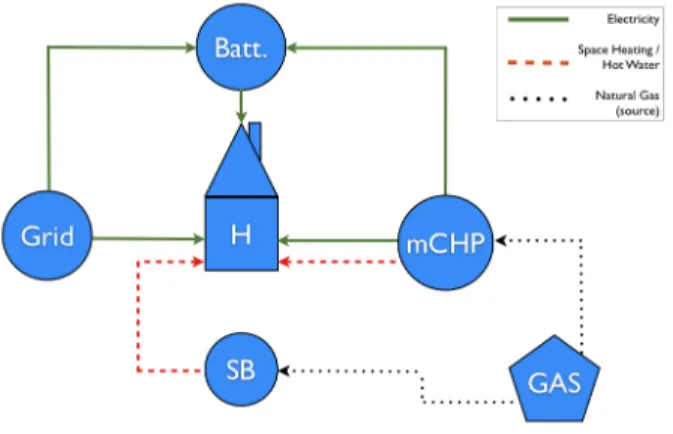
The residential system considered in this work is given in Fig. 1, however the formulation is generic enough that can be applied to any residential system with different multiple energy sources with small adjustments.
Fig. 1. Proposed System
In the system shown in Fig. 1, thermal demand of the dwelling is supplied by the mCHP device. A conventional gas-fired boiler is also considered in the system since they are already available in many households. In the figure, this boiler is shown with an acronym SB, i.e. support boiler, which represents usage aim of the boiler; it turns on in case mCHP device is closed or its generation capacity is not enough for the demand. Both devices use natural gas, which is a typical connection in many households, to generate the required heat. Electricity demand of the dwelling can be supplied by the mCHP, the national grid or the lead-acid battery which is included in the system as a storage unit.
B. Micro Combined Heat and Power (mCHP)
Micro combined heat and power devices are developed in the last decade and intended to replace conventional boilers used in residential environment. The output of these devices are same as the combined heat and power (CHP) plants which are electricity and thermal energy from a single energy source (like coal or natural gas). However, their power levels are much smaller compared to conventional CHP plants.
Mathematical model of the ICE based mCHP device used in this paper is adopted from [9]. It consists of a simple parametric model of 6 kW Cummins gas engine and it is developed according to the performance data from the manufacturer. This model incorporates dynamic efficiency values of the device thus permitting variable power output. The mCHP models used in the literature such as [4], have only full-power and part-load operation modes which limits
controllability of the device.
X = Pmg/(Pmg)max (1) HP R = 18.347X3+ 45.76X2− 39.933X + 15.7 (2) SF C = 965.6X2− 1767X + 1164.2 (3) Qmg = HP R.Pmg (4) ˙ mf = SF C.Pmg (5) According to [9], a series of tests had been conducted for critical variables of the mCHP device such as Heat-to-Power Ratio (HPR) and Specific Fuel Consumption (SFC) and an empirical formula is obtained for each critical term which all depends on a single variable, namely fraction load (X) as calculated in (1). Pmg in (1) represents electrical output of the device which will be determined by the supervisory controller and (Pmg)max is the maximum electrical power output of the device that is 6 kW. HPR and SFC of the device for the specific power output can be calculated by using (2) and (3) respectively. Qmg can be calculated by using the HPR and Pmg as shown in (4). Finally, amount of natural gas fuel consumed by the device for the corresponding time period and power is calculated with (5).
C. Battery
An electrical storage battery is known to be difficult to model due to ongoing chemical reactions inside the battery which changes the terminal voltage. The approach here is based on [10], in which certain voltage values are measured corresponding to the SOC values.
The change in the battery current and change of the battery state-of-the-charge is given in (6) and (7) respectively.
Ibatt=
Voc−pVoc2 − 4RintPbatt 2Rint
(6) SOC = SOCold−
Ibattνbattt Qbatt
(7) where Voc represents open circuit voltage across the battery, Rint is the internal resistance of the battery, νbatt is the battery charging efficiency, and Pbatt represents the amount of power either used to charge the battery or withdrawn from the battery (discharge).
D. Support Boiler
Boilers are already available in many households so they are considered as a support source besides the mCHP device for the thermal demand. Since transient operation of the mCHP device is neglected, warm-up and shut-down periods of the boiler is not considered here and a steady-state efficiency is used. Efficiency value is selected as 0.9 which is an average value from the available commercial devices. The mass flow rate of the fuel used by the boiler is calculated using (8) which is based on the approach from [11].
˙ mf =
Qboil ηb.HHV
(8) where Qboil is the required power amount from the boiler, ηb is the steady-state efficiency of the boiler and HHV is the higher heating value of the natural gas.
E. National Electricity Grid
It is assumed that, when supervisory controller requires a certain amount of power from grid, it is obtained in exact amount with no delays since grid dynamics are much faster according to our simulation step which is 5 minutes. F. Demand Cycles
A set of standard representative demand cycles for a certain occupation type, a family with 5 children, is used in this paper. This is also a common approach in automotive industry, in which drive cycle’s are used. The demand cycles used in the controller design can be found in [12].
III. CONTROLLER DEVELOPMENT
The proposed system, shown in Fig. 1, can perform without an external, supervisory controller, by manual op-eration of each component by the residents of the house. But by adopting a supervisory controller, which coordinates the operation of the devices, system performance can be increased and this performance can be obtained consistently. In order to find the optimal energy utilization of the system given a demand cycle, first a dynamic optimization study is performed using the developed mathematical model of the system in Fig 1. Then by using the optimization results, a supervisory controller is developed to be used in real-time applications.
A. Dynamic Optimization
There are various methods to solve a constrained opti-mization problem. In this work, a technique called Dynamic Programming (DP) is used because it allows possibility to consider dynamic nature of the system components. Since optimization is made for the entire horizon, it always pro-vides the globally optimum results given the demands.
Based on a formal standard representation shown in [13], we have developed a DP formulation for the residential energy management problem and it is given in (9)-(17):
J = min ~ u [GN(~xN) + N −1 X k=1 L(~x(k), ~u(k))] (9) subject to xk+1= f (xk, uk) + xk (10) x = [0.4, 0.7] (11) x0= 0.55 (12) xN ≥ 0.55 (13) u1= [−1, 1] (14) u2= [0, 1] (15) Ts= 5 min (16) N = (24 × 60)/Ts (17)
In this formulation, battery state-of-the-charge (SOC) cho-sen as only state variable, x. This is compatible with the backward facing model developed in the previous section, with battery being the only dynamic block and other sources
modelled as quasi-static. To solve the optimization problem, an initial value must be assigned to the state so it is assumed that battery starts to the day with a half full of charge (i.e 0.55) in (12), which is typical for these type of problems. Upper (i.e 0.7) and lower (i.e 0.4) bounds for the battery SOC is defined in (11) to prevent battery from depletion and overcharging, since they decrease battery life. These operational bounds are consistent with the literature, and increasing the operation zone of the battery will shorten its life-span besides it will have a small contribution to the overall efficiency of the system. Due to their increased availability plug-in HEV battery used in this residential system which has a capacity of 6 Ah. It has a small capacity compared to traditional batteries used in residential systems which generally have a capacity around 25 Ah [15]. Finally, for the numerical solution, the area formed from upper and lower bounds is discretized with 1001 steps. This number is obtained through a convergence analysis.
From (14)-(15), it can be seen that two control domains, u1 and u2, are defined. These control inputs are called as Power Split Ratio (PSR). This is a common definition in automotive industry [14], [16]. With this approach, instead of separately determining the operation modes and associated power levels of electric motor and engine in a HEV, a power split ratio is defined. Power split ratio couples this two sources by dividing power level of a one source to the total power requested by the driver. By this way DP only calculates this ratio and power level of these two sources extracted from it. For the residential energy problem,
power-Fig. 2. Control Strategy
split algorithm used in the automotive industry is extended into two layers, which can be seen in Fig. 2, since there are more energy sources in the residential system compared to HEV. In the first split in Fig. 2, the aim of the DP algorithm is determining the battery operation mode for the current demand from the occupants. Based on this decision, battery can be turned-off for the corresponding time interval or some portion of the requested power can be supplied by battery. Amount of the power requested from the house is updated according to the battery contribution, which is shown with Pgen. In the second split, The ratio of how much of the required power generation, Pgen, is taken from grid, Pgrid, and mCHP device, Pmg is decided.
The demand data used to generate the consumption pro-files was obtained from 5 minute interval measurements,
thus simulation time, Ts, is selected as 5 minutes. Dynamic optimization is performed over a day which is in total 1440 minutes. Dividing this value to the simulation time will give the optimization horizon, N, which results to 288 stages.
In this problem, it is assumed that the only objective is to reduce operational costs for the end user. However, a combined cost function is also possible and can be achieved by adding another objective like minimizing CO2emissions. Additionally, since a final state constraint is already imposed in (13), there is no need for the final cost, GN(xN). To sum up, cost function defined in (9) reduces to (18).
J = min ~ u [ N −1 X k=1 L(~x(k), ~u(k))] (18) L(~x(k), ~u(k)) = ˙mf uel(k)Cf uel+ Pgrid(k)Cgrid (19) In (19), ˙mf uelis amount of natural gas used in the matching interval and Pgrid is the amount of electricity imported. Fixed unit prices for natural gas and electricity are used which are 0.04 Euro/kWh and 0.1 Euro/kWh respectively.
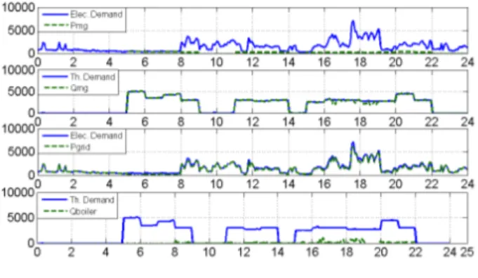
The DP formulation given in (9)-(17) is solved by using a software toolbox described detailly in [16]. Achieved optimal trajectories are given in Fig. 3. From Fig. 3, it is clearly seen that mCHP is a thermal device. This makes sense since production of electricity from mCHP device is expensive according to grid electricity, if the generated heat will not be used. From this figure it can also be concluded that besides optimal part load values, mCHP device will work three times during the day while it works only two times with a time-led controllers. This implies better utilization since extra electric power can be generated with mCHP which can decrease operational cost at the end of the day.
Fig. 3. Optimal Device Power Trajectories
B. Supervisory Control Strategy
Dynamic optimization solution provides, for a specific demand, optimal power split ratios for the devices. How-ever, since DP makes decisions not isolated with one stage but considering the future, globally optimum results found from DP cannot be used in real-time applications because the algorithm requires demand information for the selected period, in advance. Therefore a common approach in control engineering is conducted next which is investigating deci-sions of the non-causal optimal controller to obtain a causal control algorithm [16].
Although some other sensory information can be used, we will assume that our controller will only be fed with current demand information and battery SOC level in real-time application. By considering only these parameters, controller should make power splits between multiple energy sources. Instead of trying to find a rule/trend for determining PSR, as it is done in [14] for example, optimal power output of the energy sources is related with the corresponding demand information and dominant parameters for our residential energy management problem. For instance, the amount of electricity imported from national grid is determined from the surface plot given in Fig. 4. The polynomial surface fit shown in Fig. 4 is obtained by using optimal operation points found from DP results, the updated demand information (Pgen) after the battery contribution and the thermal demand (thDemand) from the dwelling. The dominant parameter, thDemand, was obvious here since in Fig. 3, it is seen that mCHP operation depends on the thermal demand.
Fig. 4. Surface fit for determining the amount of electricity imported After carefully investigating the consumption profiles pub-lished in [12], it is found that demands of a house follows a similar pattern during a particular season. Therefore, the PSR functions found above will work smoothly during the selected season even if the demands are different from the ones used in DP solution and this is verified in Section IV.
The produced PSR surface-fit functions does not consider the battery operation constraints. Because of this, battery can be depleted or overcharged depending on the actual conditions. This problem can also be seen in reference [14]. So, an additional rule set is required to keep battery between desired SOC levels. The charge sustaining algorithm for developed for this purpose is given in (20)-(24):
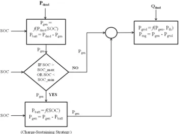
if (SOC > SOCmax) (20) Pbatt=| SOCmax− SOC | 100 × 175 (21) if (SOC < SOCmin) (22) Pbatt= − | SOC − SOCmin| 100 × 200 (23) Pgen= Pgen− Pbatt (24) The overall flow diagram developed is given in Fig. 5. In this strategy, supervisory controller is fed with current
states of the dominant parameters and demand of the users. Based on these values and using the two level PSR functions obtained from the DP analysis (such as in Fig. 4), current set-points for the energy sources are arbitrated.
Fig. 5. Proposed System
IV. SIMULATIONS
In order to evaluate and compare the performance of the developed supervisory controller, a heuristic controller is formed based on an available approach in the literature which can be found in [4]. The heuristic controller consists of hybridization of time-led and heat-led strategies which means mCHP device opens automatically two times in a day, in morning and evening periods when the consumption begins and follows the thermal load of the dwelling. And as in [15], battery is used only for catching sudden peaks in electricity demand. Results of the conducted simulations are compared based on three performance parameters from the literature, namely Primary Energy Consumption (PEC), operational costs and CO2 emissions. The latter two is self-explanatory and PEC represents amount of primary energy consumed, like natural gas, in a household including losses, which occurs due to generation and transmission of the primary energy source consumed.
A. Validation of the Controller
In this simulation, it is assumed that the demands from the dwelling is same with the demand values that are used to develop our controller. The resulting usage profile of the devices is given in Fig. 6. In this figure, blue dashed line shows optimal trajectories obtained from DP results and the solid green line represents real-time decisions made by the developed supervisory controller. The first plot in Fig. 6 shows that the electricity demand of the house satisfied perfectly by the developed controller as expected. More importantly, from the second and third plots in Fig. 6 it can be seen that supervisory controller follows the optimal results successfully, there is only minor differences between them since the polynomial surface was not a perfect fit.
Fig. 6. Daily Usage Profile of the Energy Sources
The last plot in Fig. 6 depicts SOC change of the battery. Although supervisory controller decisions follow the DP results in throughout the day, there are some small differ-ences, especially in between 10 a.m. to 15 p.m. This is due to the imperfect surface fit, however deviations are bigger according to mCHP and grid trajectories since battery SOC much more sensitive which means a small difference in Pbatt can cause a big change in SOC. However, these differences have no critical impact to the system efficiency since the battery capacity is small compared to the whole system.
TABLE I
DAILYPERFORMANCE(DEMANDS IN KWH, COSTS INEURO) Tot. Elec. Tot. Ther. Cost PEC CO2
Demand Demand Reduction
Conv. 33.7580 46.1736 4.9575 100% 100% Heuristic 33.7580 46.1736 4.7370 −3.8% −3.5%
Superv. 33.7580 46.1736 4.6489 −5.3% −5.00% Dynamic 33.7580 46.1736 4.6348 −5.6% −5.2% The performance results obtained from this simulation are given in Table I. As seen in Table I, daily cost is lowest for optimal but non-causal DP approach. This is expected since DP results gives global optimum for the system. The developed sub-optimal controller gives second best daily cost but still higher from DP. Then the heuristic control strategy and as expected conventional approach for homes produces the highest cost. It should be noted that, although decrease in cost is small, over the monthly and yearly periods the cost gain will be highly competitive even with the baseline supervisory controller developed here.
From the last column of Table I, it can be seen that a 5% of daily CO2 reduction is achieved by operating the residential system with the developed supervisory controller. This value drops to 3.5% when the energy sources in the infrastructure are not operated optimally as with heuristic controller. B. Verification of the Controller
In order to show that the developed controller performs acceptable for other demand conditions, a new set of demand cycles are used in simulations, from [12]. According to these new different demands, usage profiles of the energy sources resulted from supervisory controller and optimal DP solutions are plotted alongside in Fig. 7.
Fig. 7. Daily Usage Profile of the Energy Sources
From the first plot in Fig. 7, it can be seen that demand of the house is fully satisfied even if the demand cycle changed. Also optimal grid trajectory found from DP solution is fol-lowed with minimum deviation by the developed controller. On the other hand, although some portions are followed well, there are differences between optimal operations of the mCHP device and battery with the real-time solution. Around 10 a.m. supervisory controller decides to import more electricity from the grid compared to demand. This extra electricity used to charge the battery and since it is small battery, the capacity reached to upper bound quickly. This caused to charge sustaining strategy to step-in to prevent battery from over-charging. So battery started to discharge power which results subsequent on and off operation of mCHP device, seen in around noon time. However since the size of the battery is small, it’s effect on the system is not so high which can also be seen from the performance results.
TABLE II
DAILYPERFORMANCE(DEMANDS IN KWH, COSTS INEURO) Tot. Elec. Tot. Ther. Cost PEC CO2
Demand Demand (Euro) Reduction Conv. 14.04 46.5296 2.9979 100% 100% Heuristic 14.04 46.5296 2.7887 −5.2% −4.5%
Superv. 14.04 46.5296 2.757 −6.2% −5.5% Dynamic 14.04 46.5296 2.7159 −7.5% −6.8%
The performance results for this day is given in Table II. From Table II, it can be seen that operational costs are reduced since total electricity consumption of the house decreased compared to previous simulation. Comparing to results in Table I, the performance of the supervisory con-troller is slightly declined as expected, since it was tuned for another set of demands. In the first simulation, the developed supervisory controller performed well with only 0.2 − 0.3% deviations from the globally optimum results. However, in this simulation, this difference increases to 1.3% levels which can be still accepted within controller’s robustness limits. The developed supervisory controller still performs better than the heuristic controller with an amount of 1% in all of the performance parameters considered.
V. CONCLUSION AND FUTURE WORK In this paper, a residential energy management problem is successfully solved by a procedure adopted from an entirely different area, automotive industry. A causal supervisory controller is developed, based on dynamic programming solutions, to operate multiple energy sources available in the residential system. According to our initial simulations, an approximate 5 − 5.5% reduction is possible compared to the conventional case. It is also shown that the developed controller performs 1 − 2% better than available heuristic strategies, such as thermal load following, in terms of all three performance parameters considered here. For future work, the energy management problem will be solved by using a stochastic dynamic programming algorithm.
REFERENCES
[1] U.S. D.O.E. Energy Efficiency and Renewable Energy, The Micro-CHP Technologies Roadmap-Meeting 21st Century Residential Needs, Distributed Energy Program; December, 2003.
[2] U.S. D.O.E. Energy Efficiency and Renewable Energy, 2010 Build-ings Energy Data Book, D&R International, Ltd., Pacific Northwest National Laboratory; March, 2011.
[3] T. Ackermann and G. Andersson and L. S¨oder, ”Distributed genera-tion: a definition”, Electric Power Systems Research, vol. 57, 2001, pp 195-204.
[4] A. Peacock and M. Newborough, ”Impact of micro-CHP Systems on Domestic Sector CO2 Emissions”, Energy, vol. 32, 2007, pp
1093-1103.
[5] K. Alanne et. all, ”Techno-economic assessment and optimization of stirling engine micro-cogeneration systems in residential buildings.”, Energy Conversion and Management, vol. 51, 2010, pp 2635-2646. [6] A. Collazos and F. Marechal and C. Gahler, ”Predictive optimal
management method for the control of polygeneration systems.”, Computers and Chemical Engineering, vol. 33, 2009, pp 1584-1592. [7] M. Houwing et. all, ”Least-cost model predictive control of residential energy resources when applying µCHP”, in Proceedings of Power Tech, Lausanne, Switzerland, 2007, pp. 6.
[8] H. I. Onovwiona and V. I. Ugursal, ”Residential cogeneration systems: a review of the current technologies”, Renewable and Sustainable Energy Reviews, vol. 10, 2006, pp 389-431.
[9] H. I. Onovwiona and V. I. Ugursal and A. S. Fung, ”Modeling of internal combustion engine based cogeneration systems for residential applications”, Applied Thermal Engineering, vol. 27, 2007, pp 848-861.
[10] O. Sundstr¨om and L. Guzzella and P. Soltic., ”Optimal hybridization in two parallel hybrid electric vehicles using dynamic programming”, in 17th IFAC World Congress, 2008, pp. 4642-4647.
[11] N. J. Kelly et. all, ”Developing and testing a generic micro-combined heat and power model for simulations of dwellings and highly dis-tributed power systems”, Proceedings of the Institution of Mechanical Engineers, Part A: Journal of Power and Energy, vol. 222, 2008, pp 685-695.
[12] I. Knight et. all, European and Canadian non-HVAC Electric and DHW Load Profiles for Use in Simulating the Performance of Res-idential Cogeneration Systems, IEA Annex 42 - Technical Report; 2007.
[13] D. P. Bertsekas, Dynamic Programming and Optimal Control, Athena Scientific, 3rd edition; 2005.
[14] C.-C. Lin and H. Peng and J. Grizzle and J.M. Kang, ”Power manage-ment strategy for a parallel hybrid electric truck”, IEEE Transactions on Control Systems Technology, vol. 11, 2003, pp 839-849. [15] D. P. Jenkins and J. Fletcher and D. Kane, ”Model for evaluating
impact of battery storage on microgeneration systems in dwellings”, Energy Conversion and Management, vol. 49, 2008, pp 2413-2424. [16] O. Sundstr¨om and L. Guzzella, ”A Generic Dynamic Programming
Matlab Function”, in Proceedings of the 18th IEEE International Conference on Control Applications, Saint Petersburg, Russia, 2009, pp. 1625-1630.