RECOGNITION
a dissertation submitted to
the department of electrical and electronics
engineering
and the graduate school of engineering and science
of bilkent university
in partial fulfillment of the requirements
for the degree of
doctor of philosophy
By
Kerem Altun
Prof. Dr. Billur Barshan (Advisor)
I certify that I have read this thesis and that in my opinion it is fully adequate, in scope and in quality, as a dissertation for the degree of doctor of philosophy.
Prof. Dr. B¨ulent ¨Ozg¨uler
I certify that I have read this thesis and that in my opinion it is fully adequate, in scope and in quality, as a dissertation for the degree of doctor of philosophy.
Prof. Dr. Ergin Atalar
Prof. Dr. B¨ulent E. Platin
I certify that I have read this thesis and that in my opinion it is fully adequate, in scope and in quality, as a dissertation for the degree of doctor of philosophy.
Assist. Prof. Dr. C¸ i˘gdem G¨und¨uz Demir
Approved for the Graduate School of Engineering and Science:
Prof. Dr. Levent Onural
Director of the Graduate School of Engineering and Science
AND SIMULTANEOUS HUMAN LOCALIZATION AND
ACTIVITY RECOGNITION
Kerem Altun
Ph.D. in Electrical and Electronics Engineering Supervisor: Prof. Dr. Billur Barshan
July 2011
We consider three different problems in two different sensing domains, namely ultrasonic sensing and inertial sensing. Since the applications considered in each domain are inherently different, this thesis is composed of two main parts. The approach common to the two parts is that raw data acquired from simple sensors is processed intelligently to extract useful information about the environment.
In the first part, we employ active snake contours and Kohonen’s self-organizing feature maps (SOMs) for representing and evaluating discrete point maps of indoor environments efficiently and compactly. We develop a generic error criterion for comparing two different sets of points based on the Euclidean distance measure. The point sets can be chosen as (i) two different sets of map points acquired with different mapping techniques or different sensing modalities, (ii) two sets of fitted curve points to maps extracted by different mapping tech-niques or sensing modalities, or (iii) a set of extracted map points and a set of fitted curve points. The error criterion makes it possible to compare the accuracy of maps obtained with different techniques among themselves, as well as with an absolute reference. We optimize the parameters of active snake contours and SOMs using uniform sampling of the parameter space and particle swarm opti-mization. A demonstrative example from ultrasonic mapping is given based on experimental data and compared with a very accurate laser map, considered an absolute reference. Both techniques can fill the erroneous gaps in discrete point maps. Snake curve fitting results in more accurate maps than SOMs because it is more robust to outliers. The two methods and the error criterion are sufficiently general that they can also be applied to discrete point maps acquired with other mapping techniques and other sensing modalities.
In the second part, we use body-worn inertial/magnetic sensor units for recog-nition of daily and sports activities, as well as for human localization in GPS-denied environments. Each sensor unit comprises a tri-axial gyroscope, a tri-axial accelerometer, and a tri-axial magnetometer. The error characteristics of the sen-sors are modeled using the Allan variance technique, and the parameters of low-and high-frequency error components are estimated.
Then, we provide a comparative study on the different techniques of classify-ing human activities that are performed usclassify-ing body-worn miniature inertial and magnetic sensors. Human activities are classified using five sensor units worn on the chest, the arms, and the legs. We compute a large number of features extracted from the sensor data, and reduce these features using both Principal Components Analysis (PCA) and sequential forward feature selection (SFFS). We consider eight different pattern recognition techniques and provide a compar-ison in terms of the correct classification rates, computational costs, and their training and storage requirements. Results with sensors mounted on various lo-cations on the body are also provided. The results indicate that if the system is trained by the data of an individual person, it is possible to obtain over 99% correct classification rates with a simple quadratic classifier such as the Bayesian decision method. However, if the training data of that person are not available beforehand, one has to resort to more complex classifiers with an expected correct classification rate of about 85%.
We also consider the human localization problem using body-worn iner-tial/magnetic sensors. Inertial sensors are characterized by drift error caused by the integration of their rate output to get position information. Because of this drift, the position and orientation data obtained from inertial sensor signals are reliable over only short periods of time. Therefore, position updates from ex-ternally referenced sensors are essential. However, if the map of the environment is known, the activity context of the user provides information about position. In particular, the switches in the activity context correspond to discrete locations on the map. By performing activity recognition simultaneously with localization, one can detect the activity context switches and use the corresponding position information as position updates in the localization filter. The localization filter also involves a smoother, which combines the two estimates obtained by running the zero-velocity update (ZUPT) algorithm both forward and backward in time.
We performed experiments with eight subjects in an indoor and an outdoor en-vironment involving “walking,” “turning,” and “standing” activities. Using the error criterion in the first part of the thesis, we show that the position errors can be decreased by about 85% on the average. We also present the results of a 3-D experiment performed in a realistic indoor environment and demonstrate that it is possible to achieve over 90% error reduction in position by performing activity recognition simultaneously with localization.
Keywords: Intelligent sensing; ultrasonic sensing; inertial sensing; robot mapping; sensor error modeling; pattern recognition; wearable computing; human localiza-tion; human activity recognilocaliza-tion; simultaneous human localization and activity recognition.
ES
¸ZAMANLI KONUM BEL˙IRLEME VE AKT˙IV˙ITE
AYIRDETME ˙IC
¸ ˙IN AKILLI ALGILAMA
Kerem Altun
Elektrik ve Elektronik M¨uhendisli˘gi, Doktora
Tez Y¨oneticisi: Prof. Dr. Billur Barshan
Temmuz 2011
Algılama alanının iki ayrı kolu olan ultrasonik algılayıcılar ve eylemsizlik
algılayıcıları konularında ¨u¸c farklı problem ele alınmı¸stır. Bu iki alandaki
uygulamalar temelde birbirinden farklı oldu˘gundan, bu tez iki ana kısımdan
olu¸smaktadır. Her iki alanda da ortak olarak basit algılayıcılardan alınan ham
veriler akıllı y¨ontemlerle i¸slenerek dı¸s ortam hakkında anlamlı bilgi edinilmi¸stir.
˙Ilk kısımda, ayrık noktalardan olu¸san i¸c ortam haritalarını d¨uzenlemek ve
de˘gerlendirmek amacıyla yılan e˘grileri ve Kohonen a˘gları y¨ontemleri
uygu-lanmı¸stır. ˙Iki farklı nokta k¨umesini kar¸sıla¸stırmak amacıyla ¨Oklid uzaklı˘gına
dayanan genel bir hata ¨ol¸c¨ut¨u geli¸stirilmi¸stir. Bu nokta k¨umeleri, (i) farklı
ha-ritalama teknikleri veya algılama y¨ontemleriyle olu¸sturulmu¸s iki farklı haritanın,
(ii) farklı haritalama teknikleri ile elde edilmi¸s haritalara uyarlanan iki e˘grinin,
ya da (iii) birisi bir haritanın, di˘geri uyarlanmı¸s bir e˘grinin ¨uzerindeki
noktalar-dan olu¸sacak ¸sekilde se¸cilebilir. Bu hata ¨ol¸c¨ut¨un¨u kullanarak farklı y¨ontemlerle
elde edilmi¸s haritaları birbirleriyle ya da bir referans haritasıyla kar¸sıla¸stırmak
m¨umk¨und¨ur. Yılan e˘grileri ve Kohonen a˘glarının parametreleri, parametre
uzayını e¸sit par¸calara b¨olme ve par¸cacık s¨ur¨u optimizasyonu y¨ontemleri
kul-lanılarak eniyilenmi¸stir. Ultrasonik haritalama alanından deneysel verilere dayalı
a¸cıklayıcı bir ¨ornek verilerek mutlak referans olarak kabul edilen bir lazer
hari-tası ile kar¸sıla¸stırılmı¸stır. Her iki y¨ontem de ayrık noktalardan olu¸san
haritalar-daki bo¸slukları doldurabilmektedir. Yılan e˘grileri aykırı de˘gerlere daha duyarsız
oldu˘gundan Kohonen a˘glarından daha iyi sonu¸c vermektedir. Tanımlanan hata
¨
ol¸c¨ut¨u ve kullanılan iki y¨ontem, ba¸ska haritalama y¨ontemleri veya algılayıcılar ile
elde edilmi¸s haritalara da uygulanabilecek kadar geneldir.
˙Ikinci kısımda, v¨ucuda takılan eylemsizlik algılayıcıları ve manyetik vii
algılayıcılar yardımıyla g¨unl¨uk aktiviteler ve spor aktivitelerini ayırdetme ve
GPS olmayan ortamlarda konum belirleme ¸calı¸smaları yapılmı¸stır.
Kul-lanılan algılayıcı ¨uniteleri ¨u¸c-eksenli jiroskop, ¨u¸c-eksenli ivme¨ol¸cer ve ¨u¸c-eksenli
manyetometrelerden olu¸smaktadır. Allan varyans y¨ontemiyle bu algılayıcıların
hata karakteristikleri modellenmi¸s, d¨u¸s¨uk ve y¨uksek frekanslı hata bile¸senlerinin
parametreleri kestirilmi¸stir.
Daha sonra, v¨ucuda takılan eylemsizlik algılayıcıları ve manyetik algılayıcılar
ile farklı aktivite ayırdetme y¨ontemleri arasında kar¸sıla¸stırmalı bir ¸calı¸sma
yapılmı¸stır. Aktiviteler, g¨o˘g¨use, kollara ve bacaklara takılan be¸s adet algılayıcı
¨
unitesi ile ayırdedilmi¸stir. Algılayıcı verilerinden ¸cok sayıda ¨oznitelik ¸cıkarılmı¸s,
daha sonra bu ¨oznitelikler asal bile¸senler analizi ve ardı¸sık ¨oznitelik se¸cme
y¨ontemleri ile sayıca azaltılmı¸stır. Sekiz farklı ¨or¨unt¨u tanıma tekni˘gi ele alınmı¸s,
ve bu teknikler do˘gru ayırdetme y¨uzdesi, hesaplama maliyeti, e˘gitme ve veri
depolama gereksinimi a¸cılarından kar¸sıla¸stırılmı¸stır. V¨ucudun farklı yerlerine
takılan algılayıcılar ile elde edilen sonu¸clar sunulmu¸stur. Sonu¸clara g¨ore, belli
bir ki¸sinin verisi e˘gitme i¸cin kullanıldı˘gında, Bayes¸ci karar verme gibi basit
bir ikinci derece sınıflandırıcı ile %99’un ¨uzerinde do˘gru ayırdetme oranlarına
ula¸smak m¨umk¨und¨ur. Ancak ilgili ki¸sinin verileri e˘gitme i¸cin kullanılmıyorsa
daha karma¸sık sınıflandırıcılara ba¸svurulmalıdır. Bu durumda beklenen do˘gru
ayırdetme oranı %85 civarındadır.
Son olarak v¨ucuda takılan algılayıcılar ile insanlarda konum belirleme
prob-lemi de ele alınmı¸stır. Eylemsizlik algılayıcılarında karakteristik olarak, konum
belirleme i¸cin hız verilerinin t¨umlevi alınması nedeniyle bir sapma hatası
bulun-maktadır. Bu sapma hatası sebebiyle eylemsizlik algılayıcılarından elde edilen
konum ve y¨onelim verisi ancak kısa s¨ureler i¸cin g¨uvenilir olmaktadır. Dolayısıyla
dı¸s ortamdan referans alan algılayıcılar ile konum g¨uncellemesi yapmak
gerek-lidir. Ancak e˘ger ortamın haritası biliniyorsa, kullanıcının aktivite verisi,
konu-mu hakkında da bilgi vermektedir. ¨Ozellikle aktiviteler arası ge¸ci¸sler haritada
ayrık konumlara kar¸sılık gelmektedir. Konum belirleme ile e¸szamanlı olarak
ak-tivite ayırdetme i¸slemi de yapıldı˘gında, aktiviteler arası ge¸ci¸sleri belirlemek ve
kar¸sılık gelen konum bilgisini konum belirleme s¨uzgecinde g¨uncelleme olarak
kul-lanmak m¨umk¨und¨ur. Konum belirleme s¨uzgeci aynı zamanda d¨uzle¸stirici i¸slevi
g¨ormekte, sıfır hız g¨uncellemesi yoluyla elde edilmi¸s ileriye ve geriye y¨onelik
kes-tirimleri birle¸stirmektedir. Sekiz denek ile i¸c ve dı¸s ortamda “y¨ur¨ume,” “d¨onme”
¨
ol¸c¨ut¨u kullanılarak konum hatalarının %85 oranında azaldı˘gı g¨or¨ulm¨u¸st¨ur. Bunun
dı¸sında bir i¸c ortamda ger¸ce˘ge uygun ¨u¸c-boyutlu bir deneyin sonu¸cları
verilmek-tedir. Bu ortamda e¸szamanlı konum belirleme ve aktivite ayırdetme y¨ontemiyle
konum hatalarının %90’ın ¨uzerinde d¨uzeltilebildi˘gi g¨osterilmi¸stir.
Anahtar s¨ozc¨ukler : Akıllı algılama; ultrasonik algılayıcılar; eylemsizlik
algılayıcıları; robot haritalama; algılayıcı hata modellemesi; ¨or¨unt¨u tanıma;
giyi-lebilir bilgisayarlar; insanlarda konum belirleme; insanlarda aktivite ayırdetme; insanlarda e¸szamanlı konum belirleme ve aktivite ayırdetme.
I would like to express my gratitude to my supervisor Prof. Dr. Billur Barshan for her constant guidance throughout my Ph.D. study and her valuable comments and corrections on the manuscripts. Without her expertise and her continuous patience and understanding, completing this study would never have been possi-ble.
I would like to thank my thesis monitoring committee members Prof. Dr. Orhan Arıkan and Asst. Prof. Dr. Selim Aksoy for their supervision and guid-ance not only at the regular meetings but also any time when I consulted their expertise.
Next in line are my collaborators, Orkun Tun¸cel and Murat Cihan Y¨uksek,
to whom I am grateful for helping me with the many difficulties I encountered in this study.
I am also grateful to Aslı ¨Unl¨ugedik, Ay¸ca Arınan, Ceren Vardar, Deniz
Ker-imo˘glu, Esrag¨ul Katırcıo˘glu, G¨ozde ¨Ozcan, Hande ¨Ozcan, Harun Altun, Mahmut
Kamil Aslan, Murat Cihan Y¨uksek, Orkun Tun¸cel, ¨Ozge Topuz, Pınar Tekir,
and Temmuz Ceyhan, who took time out of their lives and participated in the experiments in this thesis. The experiments also would not have been realized without the support of Bilkent University Physical Education Unit and Bilkent University Sports Hall staff.
My roommates Tayfun K¨u¸c¨ukyılmaz and Yahya Saleh possibly deserve the
most gratitude for their patience and support during the course of my Ph.D. study.
I also owe my gratitude to C¸ i˘gdem Cengiz, who always stood by my side and
put up with me during the Ph.D. years and many more. Her unique friendship is one of the things that made this thesis possible.
I would like to thank Ay¸ca Arınan as well, not because she jokingly kept bug-ging me for a dedicated paragraph on this page, but for her ever warm friendship,
which is most valuable to me.
I would like to take this opportunity to thank my friends who have been
with me throughout my study: Ay¸se K¨u¸c¨ukyılmaz, Ba¸sar Dalkılı¸c, Cem G¨urcan,
Din¸c Yıldırım, Duygu Can, Elvin ¨Ozcan, Emre Kızılırmak, G¨ok¸cer ¨Ozg¨ur, Hivren
¨
Ozkol-Kırali, ˙Ibrahim C¸ alı¸sır, ˙Ilker ¨Unsal, Orhan Koyun, ¨Omer Talat Ayhan,
¨
Ozg¨ur Orhangazi, Selma S¸enozan, Turgut Esencan, U˘gra¸s Dalkılı¸c, U˘gur Susuz,
. . . Thanks for the fun times shared together. I am sure this list is incomplete; I also apologize for the people I possibly forgot to mention here.
And the last but definitely not the least, I would like to thank my family, who made all this possible by bringing me up to become the person that I am today. I dedicate this thesis to them.
The financial support I received throughout the study from T ¨UB˙ITAK-B˙IDEB
for four and a half years, T ¨UB˙ITAK project EEEAG-109E059 for eight months,
1 Introduction 1
I
Ultrasonic Sensing
5
2 Representing Ultrasonic Maps 6
2.1 Introduction and Previous Work . . . 6
2.1.1 Ultrasonic Sensor Signal Processing . . . 7
2.1.2 UAM Processing Methods . . . 9
2.2 Methodology . . . 12
2.2.1 The Error Criterion . . . 13
2.2.2 Active Snake Contours . . . 14
2.2.3 Kohonen’s Self-Organizing Maps . . . 18
2.2.4 Parameter Selection and Optimization Methods . . . 19
2.3 Experiments and Results . . . 22
2.3.1 Active Snake Contours . . . 27
2.3.2 Kohonen’s Self-Organizing Maps . . . 33
2.4 Discussion . . . 33
II
Inertial Sensing
40
3 Error Characterization 41 3.1 Overview and Description of MTx Sensors . . . 423.2 Experiments . . . 44
3.3 Eliminating Transients . . . 45
3.4 Allan Variance Analysis . . . 50
3.5 Magnetometer Characterization . . . 56
4 Human Activity Recognition 59 4.1 Introduction . . . 59
4.2 Classified Activities and Experimental Methodology . . . 62
4.3 Feature Extraction . . . 64
4.4 Pattern Recognition Methodology . . . 67
4.4.1 Feature Reduction and Selection . . . 67
4.4.2 Pattern Classifiers . . . 68
4.4.3 Statistical Cross-Validation Methods . . . 73
4.5 Experimental Results . . . 75
4.5.2 Selection of Validation Sets . . . 75 4.5.3 Results . . . 78 4.6 Discussion . . . 97 5 Human Localization 99 5.1 Introduction . . . 99 5.2 Experiments . . . 104 5.3 Methodology . . . 108 5.3.1 Localization . . . 109 5.3.2 Activity Recognition . . . 114
5.3.3 Simultaneous Localization and Activity Recognition . . . . 115
5.4 Results . . . 118
5.4.1 A Demonstrative 3-D Path Example . . . 128
5.4.2 Experiments on Spiral Stairs . . . 132
5.5 Discussion . . . 132
6 Summary and Conclusion 135 A Quaternions and Rotations in 3-D Space 141 A.1 Quaternion Algebra . . . 141
A.2 Euler Angles . . . 142
2.1 Structure of the 1-D SOM. . . 18
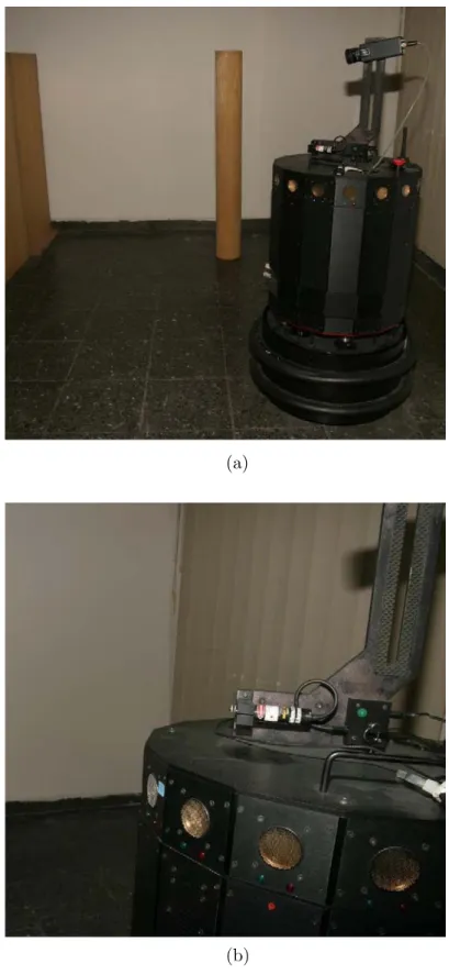
2.2 Views of the environment in Figure 2.3(a): (a) looking towards
the right, showing the top, right, and bottom walls; (b) looking towards the lower right corner, showing the right and bottom walls
in Figure 2.3(a). The cylinder is an additional feature. . . 23
2.3 (a) The raw UAM, (b) original laser map, (c) distance map with
respect to the laser data, (d) snake fitted to the laser data, (e) SOM
fitted to the laser data. . . 26
2.4 Results of snake fittings for (a) PM, (b) VT, (c) DM, (d) MP,
(e) BU (continued). . . 31
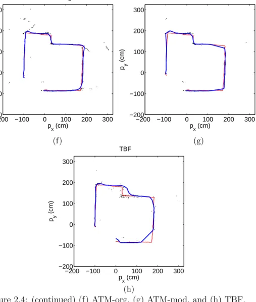
2.4 (continued) (f) ATM-org, (g) ATM-mod, and (h) TBF. . . 32
2.5 Results of SOMs for (a) PM, (b) VT, (c) DM, (d) MP, (e) BU
(continued). . . 34
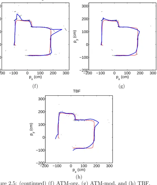
2.5 (continued) (f) ATM-org, (g) ATM-mod, and (h) TBF. . . 35
3.1 MTx 3-DOF orientation tracker
(reprinted from http://www.xsens.com/en/general/mtx). . . 42
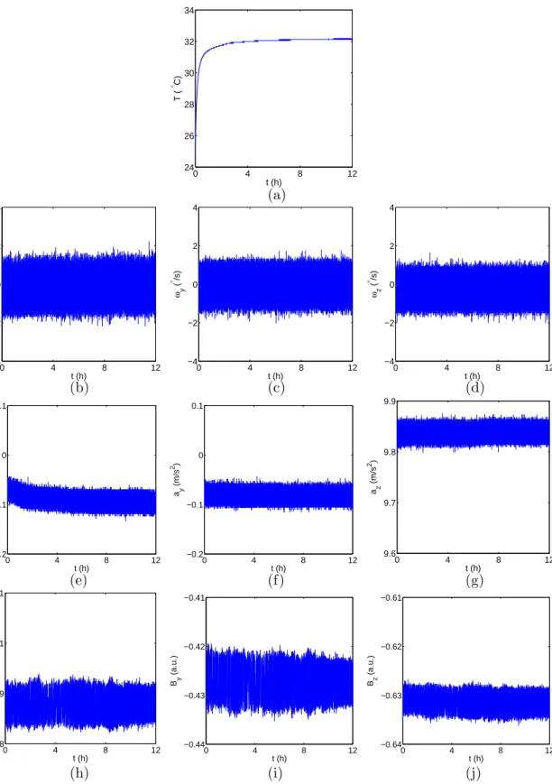
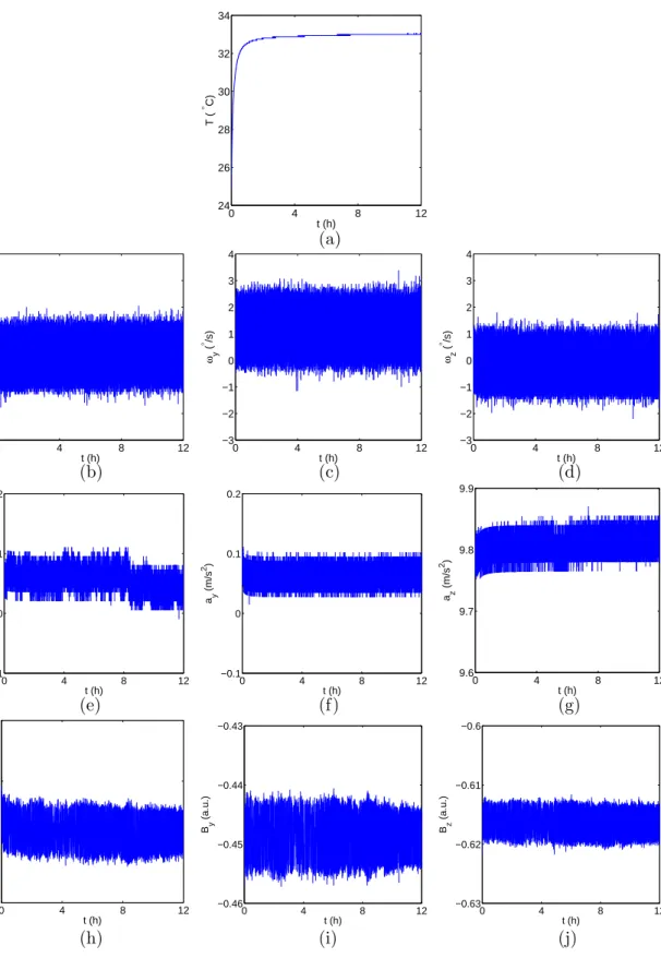
3.2 Calibrated mode data obtained from the MTx-49A53G25 unit, recorded for 12 hours. (a) Temperature, (b)-(d): x, y, z gyroscopes,
(e)-(g): x, y, z accelerometers, (h)-(j): x, y, z magnetometers. . . . 46
3.3 Calibrated mode data obtained from MTx-49A83G25 unit,
recorded for 12 hours. (a) Temperature, (b)-(d): x, y, z gyroscopes,
(e)-(g): x, y, z accelerometers, (h)-(j): x, y, z magnetometers. . . . 47
3.4 Gyroscope signal after applying the moving average filter. . . 48
3.5 Sample Allan variance plot (adopted from [57]). . . 52
3.6 Allan variance plots for x, y, z gyroscopes of the (a)
MTx-49A53G25 unit, (b) MTx-49A83G25 unit, and x, y, z
accelerom-eters of (c) MTx-49A53G25 unit, (b) MTx-49A83G25 unit. . . 54
3.7 Allan variance, autocorrelation, and PSD plots of
magnetome-ter residuals for the 49A53G25 (left column), and
MTx-49A83G25 (right column) units. . . 57
4.1 Positioning of Xsens sensor modules on the body. . . 63
4.2 (a) and (b): Time-domain signals for walking and basketball,
re-spectively; z axis acceleration of the right (solid lines) and left arm (dashed lines) are given; (c) and (d): autocorrelation functions of the signals in (a) and (b); (e) and (f): 125-point DFT of the signals
in (a) and (b), respectively. . . 66
4.3 (a) All eigenvalues (1,170) and (b) the first 50 eigenvalues of the
covariance matrix sorted in descending order. . . 76
4.4 Scatter plots of the first five features selected by PCA. . . 77
4.5 Scatter plots of the first three features selected using BDM and
4.6 ROC curves for (a) BDM, (b) LSM, (c) k-NN, and (d) ANN using RRSS cross validation. In parts (a) and (c), activities other than A7 and A8 are all represented by dotted horizontal lines at the top
where the TPR equals one. . . 91
5.1 Strap-down INS integration. . . 101
5.2 The path followed in first four experiments (all dimensions in m). 104
5.3 The path followed in the second set of experiments (all dimensions
in m). . . 105
5.4 Top views of global and the sensor-fixed coordinate frames, before
and after the alignment reset operation is performed. . . 108
5.5 Block diagram for the first processing step. . . 109
5.6 The human gait cycle (figure from
http://www.sms.mavt.ethz.ch/research/projects/prostheses/GaitCycle).111
5.7 (a) Original heading signal (dashed blue line) and swing-stance
phase indicator variable (solid red line) superimposed; (b) origi-nal heading sigorigi-nal (dashed blue line) and corrected heading sigorigi-nal (solid red line). . . 112
5.8 Optimal combination (solid blue line) of the forward (dash-dot
green line) and backward (dashed magenta line) estimates. The thin solid red line shows the true path. . . 118
5.9 Sample reconstructed paths for experiments (a) 1, (b) 3, (c) 5,
(d) 8, (e) 9, (f) 11, with (solid blue line) and without (dashed green line) activity recognition cues. The true path is indicated
with the thin red line. . . 120
5.10 Average error values for all experiments with and without applying activity recognition position updates. . . 121
5.11 Incorrectly reconstructed paths caused by (a) incorrect activity recognition, and (b) offsets in sensor data. . . 123 5.12 Sample reconstructed paths for experiments (a) 5, (b) 8, (c) 9,
(d) 11, with (solid blue line) and without (dashed green line) activ-ity recognition cues on the whole map. The true path is indicated
with thin red line. . . 124
5.13 Average error values for the experiments 5–11 with and without activity recognition position updates when the whole map is used. 126 5.14 Sample reconstructed path for the 3-D experiment. . . 130
5.15 Sample reconstructed path for the spiral stairs. . . 133
2.1 UAM processing techniques used in this study and their indices. . 9
2.2 Best parameter values found by (i) uniform sampling of the
pa-rameter space, and (ii) initializing PSO with the best papa-rameters
of (i). . . 24
2.3 Values of some experimental quantities. . . 27
2.4 Error values (in pixels) for snake curve fitting and SOM using
parameters found by uniform sampling of the parameter space. . . 29
2.5 Error values (in pixels) for snake curve fitting and SOM using PSO
parameters. . . 29
2.6 Computation times for fitting snake curves and SOM for a given
parameter set. . . 37
3.1 Alignment matrices, gain matrices, and bias vectors for the (a)
MTx-49A53G25 and (b) MTx-49A83G25 units. . . 44
3.2 Fitted parameter values for the MTx-49A53G25 unit. . . 49
3.3 Fitted parameter values for the MTx-49A83G25 unit. . . 49
3.4 Percentages of the samples inside ±2σRxx bounds for both MTx
units. . . 50
3.5 PSD and Allan variance representations of various noise types. . . 53
3.6 Velocity/angle random walk coefficients obtained from Allan
vari-ance plots. The units are (◦/√h) for gyroscopes and (m/s/√h) for
accelerometers. . . 55
3.7 Bias instability values obtained from Allan variance plots. The
units are (mg) for accelerometers and (◦/h) for gyroscopes. . . . 55
4.1 Subjects that performed the experiments and their profiles. . . 63
4.2 Correct differentiation rates for all classification methods and three
cross-validation techniques. The results of the RRSS and P -fold cross-validation techniques are calculated over 10 runs, whereas
those of L1O are over a single run. . . 78
4.3 Confusion matrix for BDM (P -fold cross validation, 99.2%). . . . 81
4.4 Confusion matrix for RBA (P -fold cross validation, 84.5%). . . . . 82
4.5 Confusion matrix for LSM (P -fold cross validation, 89.6%). . . . . 83
4.6 Confusion matrix for the k-NN algorithm for k = 7 (P -fold cross
validation, 98.7%). . . 84
4.7 Confusion matrix for DTW1 (P -fold cross validation, 83.2%). . . . 85
4.8 Confusion matrix for DTW2 (P -fold cross validation, 98.5%). . . . 86
4.9 (a) Number of correctly and incorrectly classified motions out of
480 for SVMs (P -fold cross validation, 98.8%); (b) same for ANN
(P -fold cross validation, 96.2%). . . . 87
4.10 First five features selected by SFFS using BDM, LSM, and k-NN
4.11 Correct classification percentages using the first five features
ob-tained by PCA using BDM, LSM, and k-NN. . . . 89
4.12 Pre-processing and training times, storage requirements, and pro-cessing times of the classification methods. The propro-cessing times
are given for classifying a single feature vector. . . 93
4.13 All possible sensor combinations and the corresponding correct classification rates for some of the methods using P -fold cross val-idation (T: torso, RA: right arm, LA: left arm, RL: right leg, LL:
left leg). . . 95
4.14 Best combinations of the subjects and correct classification rates
using P -fold cross validation. . . . 96
4.15 Best combinations of the subjects and correct classification rates
using subject-based L1O. . . 97
5.1 Total path lengths of the experiments. . . 106
5.2 Profiles of the eight subjects. . . 107
5.3 Parameter values used in the experiments. . . 119
5.4 Error values without activity recognition updates (in cm/m). . . . 119
5.5 Error values with activity recognition updates (in cm/m). . . 121
5.6 Averaged position errors at the position update locations (in cm/m).122
5.7 Error values with activity recognition updates using the whole map
(in cm/m). . . 125
5.8 Error values with activity recognition updates using the whole
map, after defining more WT switch locations (in cm/m). . . 127
5.10 Walking-to-turning (WT) and walking-to-stairs (WZ) activity switch locations. . . 130
List of Abbreviations
ANN Artificial Neural Networks
ATM Arc-Transversal Median
BDM Bayesian Decision Making
BU Bayesian Update
CCPDF Class-Conditional Probability Density Function
DFT Discrete Fourier Transform
DM Directional Maximum
DOF Degrees-of-Freedom
DOI Direction-of-Interest
DTW Dynamic Time Warping
FPR False Positive Rate
GPS Global Positioning System
GSM Global System for Mobile Communications
IMU Inertial Measurement Unit
INS Inertial Navigation System
k-NN k-Nearest Neighbor
L1O Leave-One-Out
LOS Line of Sight
LSM Least Squares Method
MEMS Micro Electro-Mechanical Systems
MP Morphological Processing
PCA Principal Components Analysis
PDR Pedestrian Dead Reckoning
PM Point Marking
PSD Power Spectral Density
PSO Particle Swarm Optimization
RCD Regions of Constant Depth
RFID Radio-Frequency Identification
ROC Receiver Operating Characteristics
RRSS Repeated Random Sub-Sampling
SBFS Sequential Backward Feature Selection
SFFS Sequential Forward Feature Selection
SOM Kohonen’s Self-Organizing Map
SVM Support Vector Machines
TBF Triangulation-Based Fusion
TOF Time-of-Flight
TPR True Positive Rate
UAM Ultrasonic Arc Map
VT Voting and Thresholding
WiFi Wireless Fidelity
WS Walking-to-Standing
WT Walking-to-Turning
WZ Walking-to-Stairs
List of Symbols
aG acceleration vector in the local navigation frame
aS acceleration vector in the sensor frame
A snake evolution matrix
b(t) slow-varying bias model
b manufacturer-supplied bias vector
B bias instability coefficient
c1, c2 bias model coefficients
d(·, ·) Euclidean distance between two points
d distance traveled on the xy-plane
dz distance traveled on the z-direction
DQ(·) Euclidean distance map of point set Q
Eext external energy of the snake
Eint internal energy of the snake
Esnake total energy of the snake
E(P−Q) average distance between point sets P and Q
f0 sinusoidal noise frequency
G gain matrix
g gravitational acceleration of the Earth
gBest global best value in PSO
gn global best position in PSO
Istep indicator variable of stance/swing phase
I identity matrix
J (x) objective function
kλ learning rate decay coefficient
kσ standard deviation decay coefficient
K(·, ·) SVM kernel function
KT conversion matrix
M misalignment matrix
n iteration number
Nk number of points on the kth snake of SOM curve
Ns inertial/magnetic sensor signal length
o output value of neurons in ANN
O matrix representing higher-order modeling
px(s), py(s) x and y coordinates of snake or SOM curve
pBest previous best value in PSO
pn previous best position in PSO
P finite set of discrete points
Pws,i covariance matrix for the ith WS switch location
Pwt,j covariance matrix for the jth WT switch location
Pξ covariance matrix of the initial condition
qc correlated noise coefficient
qGS orientation of the sensor frame with respect to
the local navigation frame
Q finite set of discrete points
Q process noise covariance
r raw A/D converter reading
Rss(∆) autocorrelation of signal s
ˆ
Rss(∆) autocorrelation estimate (unbiased)
˜
Rss(∆) autocorrelation estimate (biased)
Rθ rotation matrix on the plane
s arc length parameter
s[i], si ith sample of signal s
s measured inertial/magnetic signal
Sk kth snake or SOM curve fitted
Ss(f ) power spectral density
SDF T(k) discrete Fourier transform
t target output value in ANN
T bias model time constant
Tc correlated noise correlation time
u input to the localization state equation
U (·) potential function
w inertia weight in PSO
w ANN weight
x, y, z coordinates of position
x position of a particle in PSO
˙x velocity of a particle in PSO
α elasticity parameter
β rigidity parameter
γ Euler step size
∆ first-order difference operator
ζ SVM kernel parameter
κ external force weight
λ learning rate
µs mean of signal s
µws,i ith WS switch location
µwt,j jth WT switch location
µξ mean value of the initial condition
ξ state vector (position)
ˆ
ξf state vector forward estimate
ˆ
ξb state vector backward estimate
ˆ
ξ combined estimate
σ standard deviation
σ(τ ) Allan standard deviation
σ2 variance
σ2(τ ) Allan variance
σK rate random walk coefficient
σN white noise power
σQ quantization noise coefficient
Σf covariance matrix of the forward estimate
Σb covariance matrix of the backward estimate
Σ covariance matrix of the combined estimate
τ averaging time
ψ yaw angle
ω angular velocity
ΩT angular speed threshold
Introduction
Sensing and perception are two key research areas in robotics as well as in human-computer interaction. These two terms are linked through intelligent processing, where raw sensor data should be processed intelligently to gain information about the environment. In this context, sensing should be regarded as a low-level pro-cess, where various physical quantities are measured using an electronic device. Correct processing and interpretation of the measured quantities by an intelli-gent aintelli-gent such as a robot or a computer leads to perception, which stands for a higher-level understanding of the environment by the agent. The perceived infor-mation about the environment can then be used by the agent for many purposes; for example, navigation or mapping if the agent is a mobile robot, or if the agent is a wearable system worn by a human (who is part of the environment), the perceived information can be used in human-computer interaction.
The concepts in this thesis are situated at the boundary between sensing and perception. We use simple low-cost sensors to begin with, and apply intelligent processing methods to extract meaningful information from sensor data. We consider three different applications in two different sensing domains, namely ultrasonic sensing and inertial sensing. Since the applications considered in each domain are inherently different, this thesis is composed of two main parts. We motivate these applications in the rest of this chapter, and refer the reader to the corresponding chapter and our related publications for detailed descriptions
of the applied methods.
Part I includes Chapter 2, where we use active snake contours and Kohonen’s self-organizing feature maps to represent the ultrasonic map data more compactly and efficiently. This part is based on the publications [1, 2, 3, 4]. In this chapter, we fit curves to the processed ultrasonic maps using these two methods, and eliminate the undesired artifacts on the map caused by problems inherent to ultrasonic sensors such as multiple and higher-order reflections and cross-talk. The concepts in this part can be applied to a discrete point map obtained with other sensing modalities as well, such as infrared or laser, in order to eliminate undesired outlier points while keeping the structure of the map.
Part II includes Chapters 3, 4, and 5. In this part, we address two problems involving inertial sensors in wearable systems: human activity recognition and localization. We also combine these problems in Chapter 5, using activity recog-nition information to aid in localization. In Chapter 3, we first use the Allan variance method to model the low- and high-frequency components of the noise in inertial sensor data. The transients are removed using a curve fitting proce-dure before the Allan variance method is applied. These error models can be used in navigation applications where the gyroscope and accelerometer outputs are integrated in a strap-down navigation system. Chapter 4 is based on the publications [5, 6]. In this chapter, we use body-worn inertial/magnetic sensor units and apply pattern recognition techniques to determine the activity context of the user. For our preliminary studies on activity recognition, the reader is re-ferred to [7, 8], which is not included in this thesis. In [7, 8], we use two uniaxial gyroscopes worn on the leg to distinguish between eight leg motions. We report our classification results by considering various pattern recognition and feature selection techniques, which forms a basis for our studies on the recognition of daily and sports activities. Human activity recognition has many applications, some of them being biomechanics, home-based rehabilitation, remote monitoring of the elderly people and children, detecting and classifying falls, and motion cap-ture and animation. With the advancement of mobile technology, inertial sensing equipment are standardized in new generation mobile phones. Activity recogni-tion methods implemented in these phones enable the phone to have informarecogni-tion
about the user, which can help in several human-computer interaction scenarios. Another increasingly popular application in mobile technology is location-based services [9], where the phone user is provided with different services depending on his/her location estimated with GPS or other absolute sensing mechanisms in-tegrated in the mobile phone. Inertial sensors can be used for aiding localization as well, which is the subject of Chapter 5.
In Chapter 5, we consider the problem of localization using inertial sensors only. Due to the integration operations involved in estimating position and orien-tation from inertial sensor data, the drift errors in the position and orienorien-tation are unavoidable. Since these errors are cumulative, the overall error grows without bound over long periods of time. Therefore, position data from other absolute sensing modalities are usually utilized in order to correct the position estimates from inertial sensors. However, in this chapter, we use activity recognition in-formation simultaneously with the localization algorithm and a given map of the environment to provide position updates. If the map is known, activity recogni-tion informarecogni-tion and especially switches between the activity context give impor-tant information about the location. For example, in an indoor setting, switching from walking to ascending stairs means that the person is at one of the stair areas of the building, just having started ascending stairs. This usually corresponds to a few discrete locations on the given map. By simultaneously performing ac-tivity recognition and localization, position updates provided by acac-tivity context switch detection can be used in the localization process, and accurate localization can be achieved without resorting to externally referenced sensing methods. Our method can especially be used in underground mines, where usually no absolute position sensing infrastructure is present. It can also aid the localization perfor-mance in outdoor environments to reduce the GPS positioning accuracy (usually in the order of several meters) or in urban indoor environments to reduce the GSM positioning accuracy (usually in the order of 100 meters). Simultaneous activity recognition and localization have not been done before as it is handled here. We were able to find only two papers in the previous work, one of which also uses data from externally referenced sensors (GPS) and the other uses activ-ity recognition cues not for position updates, but to detect human gait phases.
The references are provided in the chapter text. Therefore, to our knowledge, the work in this chapter is the first in literature to perform activity recognition and localization simultaneously, using activity recognition cues for position updates, with only using body-worn inertial and magnetic sensors.
In Chapter 6, we summarize our results and provide future research directions for the applications considered in this thesis.
Ultrasonic Sensing
Representing and Evaluating
Ultrasonic Maps Using Active
Snake Contours and Kohonen’s
Self-Organizing Feature Maps
2.1
Introduction and Previous Work
Autonomous robots must be aware of their environment and interact with it through sensory feedback. The potential of simple and inexpensive sensors should be fully exploited for this purpose before more expensive alternatives with higher resolutions and resource requirements are considered. Ultrasonic sensors have been widely employed because of their accurate range measurements, robustness, low cost, and simple hardware interface. We explore the limits of these sensors in mapping through intelligent processing and representation of ultrasonic range measurements. When coupled with intelligent processing, ultrasonic sensors are a useful alternative to more complex laser and camera systems. Furthermore, it may not be possible to use the latter in some environments due to surface char-acteristics or insufficient ambient light. Despite their advantages, the frequency
range at which air-borne ultrasonic transducers operate is associated with a large beamwidth that results in low angular resolution and uncertainty at the location of the echo-producing feature. Furthermore, ultrasonic range maps are char-acterized by echo returns resulting from multiple and higher-order reflections, cross-talk between transducers, and noise. These maps are extremely inefficient and unintuitive representations of even the simplest environmental structures that generate them. Thus, having an intrinsic uncertainty of the actual angular direction of the range measurement and being prone to the various phenomena mentioned above, a considerable amount of processing, interpretation, and mod-eling of ultrasonic data is necessary.
In this study, we propose two approaches for efficiently representing and eval-uating discrete point maps of an environment obtained with different ultrasonic arc map (UAM) processing techniques. The first approach involves fitting active snake contours [10] to the processed UAMs. Snakes are inherently closed curves suitable for representing the features of an environment on a given map. The sec-ond approach involves fitting Kohonen’s self-organizing feature maps (SOMs) [11] (which can be implemented as either closed or open curves, using the positions of map points as input features) to an artificial neural network. In ultrasonic maps, gaps frequently occur where a number of contiguous points are marked as empty despite the fact that they are occupied. Both approaches generate para-metric curves that fill the erroneous gaps between map points and allow the map to be represented and stored more compactly and smoothly, with fewer points and using a limited number of parameters. These methods also make it possible to compare the accuracy of maps acquired with different techniques or sensing modalities among themselves, as well as to an absolute reference.
2.1.1
Ultrasonic Sensor Signal Processing
In earlier work, there have been two basic approaches to representing ultrasonic
data: feature based and grid based. Grid-based approaches do not attempt
to make difficult geometric decisions early in the interpretation process, unlike feature-based approaches that extract the geometry of the sensor data as the first
step. As a first attempt to feature-based mapping, several researchers have fitted line segments to ultrasonic data as features that crudely approximate the room geometry [12, 13, 14]. This approach proves to be difficult and brittle because straight lines fitted to time-of-flight (TOF) data do not necessarily match or align with the world model, and may yield many erroneous line segments. Improving the algorithms for detecting line segments and including heuristics do not re-ally solve the problem. A more physicre-ally meaningful representation is to use regions of constant depth (RCDs) as features, which are circular arcs from specu-larly reflecting surfaces that are natural features of the raw ultrasonic TOF data. These arcs were first reported in [15] and further elaborated on in [16]. They are obtained by placing a small mark along the line of sight (LOS) at the range cor-responding to the measured TOF value. In specularly reflecting environments, an accumulation of such marks usually produces arc-like features. As a more general approach that is not limited to specularly reflecting surfaces, the angular uncertainty in the range measurements has been represented by UAMs [17] that preserve more information (see Figure 2.3(a) for a sample UAM). Note that the arcs in the UAM are uncertainty arcs and different than the arcs corresponding to RCDs. The UAMs are obtained by drawing arcs spanning the beamwidth of the sensor at the measured range, representing the angular uncertainty of the object location and indicating that the echo-producing object can lie anywhere on the arc. The probability of the reflection point being in the middle of the arc is the largest, symmetrically decreasing towards the sides. In the literature, the proba-bility of occupancy along the arc has been modeled by Elfes heuristically [18, 19]. Thus, when the same transducer transmits and receives, all that is known is that the reflection point lies on a circular arc of radius r, with a larger probability in the middle of the arc. More generally, when one transducer transmits and another receives, it is known that the reflection point lies on the arc of an ellipse whose focal points are the transmitting and receiving elements. The arcs are tangent to the reflecting surface at the actual point(s) of reflection.
Completely specular and completely diffuse (Lambertian) reflection are both idealizations corresponding to the two extreme cases of the actual spectrum of real reflection characteristics. These two extrema are unreachable in practice
and many real environments are, in fact, compositions of both specularly and diffusely reflecting elements. Compared to RCDs, constructing UAMs is more generally applicable in that they can be generated for environments comprised of both specularly and diffusely reflecting surfaces as is the case for many typical indoor environments. On the other hand, RCDs are structures that occur in environments where specular reflections are dominant. In earlier work, techniques based on the Hough transform have been applied to detect line and point features from arcs for both airborne and underwater ultrasonic data [20, 21].
2.1.2
UAM Processing Methods
Since the UAM is generated by drawing an arc for each received echo, the resulting map has many redundant points, as well as artifacts caused by cross-talk, and multiple and higher-order reflections (Figure 2.3(a)). Several techniques exist in the literature that can be used to process the UAMs. These techniques, listed in Table 2.1, are described in this section.
Table 2.1: UAM processing techniques used in this study and their indices.
k UAM processing technique
1 point marking (PM) [15]
2 voting and thresholding (VT) [22]
3 directional maximum (DM) [19]
4 morphological processing (MP) [17]
5 Bayesian update (BU) [18]
6 arc-transversal median (ATM-org) [23]
7 modified ATM (ATM-mod) [19]
8 triangulation-based fusion (TBF) [24]
2.1.2.1 Point Marking (PM)
This is the simplest approach, where a mark is placed along the LOS at the mea-sured range [15]. This method produces reasonable estimates for the locations of objects if the arc of the cone is small. This can be the case at higher frequencies
of operation where the corresponding sensor beamwidth is small or at nearby ranges. Since every arc is reduced to a single point, this technique cannot elimi-nate any of the outlying TOF readings. The resulting map is usually inaccurate with large angular errors and artifacts.
2.1.2.2 Voting and Thresholding (VT)
In this technique, each pixel stores the number of arcs crossing that pixel, resulting in a 2-D array of occupancy counts for the pixels [22]. By simply thresholding this array and zeroing the pixels lower than the threshold, artifacts can be eliminated and the map is extracted.
2.1.2.3 Directional Maximum (DM)
This technique is based on the idea that in processing the acquired range data, there is a direction-of-interest (DOI) associated with each detected echo. Ideally, the DOI corresponds to the direction of a perpendicular line drawn from the sensor to the nearest surface from which an echo is detected. However, in practice, due to the angular uncertainty of the object position, the DOI can be approximated as the LOS of the sensor when an echo is detected. Since prior information on the environment is usually unavailable, the DOI needs to be updated while sensory data are being collected and processed on-line [19].
In the implementation, the number of arcs crossing each pixel of the UAM is counted and stored, and a suitable threshold value is chosen, exactly the same way as in the VT method. The novelty of the DM method is the processing done along the DOI. Once the DOI for a measurement is determined using a suitable procedure, the UAM is processed along this DOI as follows: The array of pixels along the DOI is inspected and the pixel(s) exceeding the threshold with the maximum count is kept, while the remaining pixels along the DOI are zeroed out. If there exist more than one maxima, the algorithm takes their median (if the number of maxima is odd, the maxima in the middle is taken; if the number
is even, one of the two middle maxima is randomly selected). This way, most of the artifacts of the UAM can be removed.
2.1.2.4 Morphological Processing (MP)
The processing of UAMs using morphological operators was first proposed in [17]. This approach exploits neighboring relationships and provides an easy to imple-ment yet effective solution to ultrasonic map building. By applying binary mor-phological operators, one can eliminate the artifacts of the UAM and extract the surface profile.
2.1.2.5 Bayesian Update Scheme for Occupancy Grids (BU)
Occupancy grids were first introduced by Elfes, and a Bayesian scheme for up-dating their probabilities of occupancy and emptiness was proposed in [18] and verified by ultrasonic data. Starting with a blank or completely uncertain occu-pancy grid, each range measurement updates the probabilities of emptiness and occupancy in a Bayesian manner. The reader is referred to [18] for a detailed description of the method and [19] for its implementation in this work.
2.1.2.6 Triangulation-Based Fusion (TBF)
The TBF method is primarily developed for accurately detecting the edge-like features in the environment based on triangulation [24]. The triangulation equa-tions involved are not suitable for accurately localizing planar walls.
Unlike the previously introduced grid-based techniques, the TBF method ex-tracts the features of the environment by using a geometric model suitable for edge-like features. In addition, TBF considers a sliding window of ultrasonic scans where the number of rows of the sliding window corresponds to the number of ultrasonic sensors fired, and the number of columns corresponds to the num-ber of most recent ultrasonic scans to be processed by the algorithm. TBF is
focused on detection of edge-like features located at ≤ 5 m. The other methods consider all of the arcs in the UAM corresponding to all ranges, and are suitable for detecting all types of features.
2.1.2.7 Arc-Transversal Median (ATM)
The ATM algorithm requires both extensive bookkeeping and considerable amount of processing [23]. For each arc in the UAM, the positions of the in-tersection(s) with other arcs, if they exist, are recorded. For arcs without any intersections, the mid-point of the arc is taken to represent the actual point of reflection (as in PM). If the arc has a single intersection, the algorithm uses the intersection point as the location of the reflecting object. For arcs with more in-tersections, the median of the positions of the intersection points with other arcs is chosen to represent the actual point of reflection. In [23], the median operation is applied when an arc has three or more intersection points. If there is an even number of intersections, the algorithm uses the mean of the two middle values (except that arcs with two intersections are ignored). It can be considered as a much improved version of the PM approach.
We have also implemented a modified version of the algorithm (ATM-mod) where we ignored arcs with no intersections. Furthermore, since we could not see any reason why arcs with two intersections should not be considered, we took the mean of the two intersection points.
2.2
Methodology
One of the purposes of this study is to evaluate and compare the performances of different UAM processing techniques, by fitting active snake contours and SOMs to the map data. To establish a quantitative measure of the performance, we first define a generic error criterion between two sets of points, based on the Euclidean distance.
2.2.1
The Error Criterion
Let P ⊂ R3 and Q ⊂ R3 be two finite sets of arbitrary points with N1 points in
set P and N2 points in set Q. We do not require the correspondence between the
two sets of points to be known. Each point set could correspond to either (i) a set of map points acquired by different mapping techniques or different sensing modalities (e.g., laser, ultrasonic, or infrared map points), (ii) discrete points corresponding to an absolute reference (the true map), or (iii) some curve (in 2-D) or shape (in 3-D) fit to the map points (e.g., polynomials, snake curves, or spherical caps). The absolute reference (or ground truth) could be an available true map or plan of the environment or could be acquired by making range or time-of-flight measurements through a very accurate sensing system.
The well-known Euclidean distance d(pi, qj) : R3 × R3 → R≥0 of the ith
point in set P with position vector pi = (pxi, pyi, pzi)T to the jth point qj =
(qxj, qyj, qzj)T in set Q is given by:
d(pi, qj) =
√
(pxi− qxj)2+ (pyi− qyj)2+ (pzi− qzj)2 (2.1)
where i∈ {1, . . . , N1} and j ∈ {1, . . . , N2}.
In [25], three different metrics to measure the similarity between two sets of points are considered and compared, each with certain advantages and disadvan-tages. In this work, we use the most favorable of them to measure the closeness or similarity between sets P and Q:
E(P−Q)= 1 2 ( 1 N1 N1 ∑ i=1 min qj∈Q {d(pi, qj)} + 1 N2 N2 ∑ j=1 min pi∈P {d(pi, qj)} ) (2.2)
According to this criterion, we take into account all points in the two sets and find the distance of every point in set P to the nearest point in set Q and average them, and vice versa. The two terms in Equation (2.2) are also averaged, so that the criterion is symmetric with respect to P and Q. If the two sets of points are completely coincident, the average distance between them will be zero. If one set is a subset of the other, there will be some error. Had an asymmetric criterion been employed, say, including only the first (or the second) term in
Equation (2.2), the error would have been zero when P ⊂ Q (or Q ⊂ P ). Gaps occurring in the maps and sparsity are penalized by this error criterion, resulting in larger errors on average.
The error criterion we propose is sufficiently general that it can be used to compare any two arbitrary sets of points. This makes it possible to compare the accuracy of discrete point maps acquired with different techniques or sensing modalities with an absolute reference, as well as among themselves, both in 2-D and 3-D. When curves or shapes (e.g., lines, polynomials, snakes, spherical or elliptical caps) are fitted to the map points, the criterion proposed here also enables us to assess the goodness of fit of the curve or shape to the map points. In other words, a fitted curve or shape comprised of a finite number of points can be treated in exactly the same way.
2.2.2
Active Snake Contours
A snake, or an active contour, first introduced by Kass et al. [10], can be de-scribed as a continuous deformable closed curve. Active snake contours have been commonly used in image processing for edge detection and segmenta-tion [10, 26, 27, 28], and have been mostly classified into three categories [29]:
• point-based snakes, where the curve is represented as a collection of discrete points,
• parametric snakes, where the curve is described using combinations of basis functions, and
• geometric snakes, where the curve is represented as a level set of a higher-dimensional surface.
This classification is not universal and many authors categorize snakes merely into two, namely parametric and geometric, with the first category stated above considered a special kind of parametric snake. The snake used in this study
belongs to the first category. The variants of snakes are analyzed in a unified manner in [30].
We define a snake as a parameterized closed curve v(s) = [px(s), py(s)]T,
s∈ [0, 1], where px(s) and py(s) are functions representing the Cartesian
coordi-nates of the snake in 2-D and s is the normalized arc length parameter of the snake curve. This parameterization is dimensionless. The deformation of the snake is controlled by internal and external forces. Internal forces impose elastic-ity and rigidelastic-ity constraints on the curve, whereas external forces stretch or shrink the curve to fit to the image data. The total energy of the snake curve is given by the functional
Esnake =
∫ 1
0
[Eint(v(s)) + Eext(v(s))] ds (2.3)
The internal energy component is given by
Eint(v(s)) = 1 2 ( α d(v(s)) ds 2+ β d 2(v(s)) ds2 2 ) (2.4)
where α is the elasticity parameter and β is the rigidity parameter, and ∥·∥
denotes the 2-norm. The first derivative term in Equation (2.4) penalizes long
curves, whereas the second derivative term penalizes sharp curvatures. This
internal energy definition is used in many applications, possibly with varying α(s) and β(s). The use of other internal energy expressions is not very common.
The external energy component is denoted by Eext(v(s)) = U (v(s)), where U
is a potential function that depends on the image data. In general, the potential function can be selected in different ways, depending on the application. However, it must be at minimum on the edges of the image if the snake is to be used for edge detection, segmentation, or finding the boundaries of an environment as in our application. Kass et al. suggest using the negative of the image gradient magnitude as a potential function [10]. However, this is only feasible if the snake is initialized close to the image boundaries, otherwise the snake curve would be stuck in local minima or a flat region of the potential function. Filtering the image with a Gaussian low-pass filter is also suggested in the same paper to increase the capture range of the snake, but this causes the edges to become
blurry, thus reducing map accuracy. In black-on-white and gray-level images, the image intensity can be used as the potential function, either in binary form or convolved with a Gaussian blur [27]. Obviously, this method also suffers from the drawbacks stated above. Another solution, proposed in [28], is using a distance map as a potential function to increase the capture range of the contour, which is the approach used in this study.
In this work, we chose to use a potential function for the external energy term based on the Euclidean distance map, as suggested in [28]. Although our problem is in 2-D, let us first make a more general definition of a distance map in 3-D.
2.2.2.1 Euclidean Distance Map
Let Q ⊂ R3 be a finite set of arbitrary points. For all points p of the mapped
region, we define a distance map DQ(p) : R3 → R≥0 between a point p and set
Q as the minimum of the Euclidean distances of that point to all the points in the set Q. That is,
DQ(p) = min
qj∈Q
{d(p, qj)} j ∈ {1, . . . , N2} (2.5)
where qj is the position vector of the jth point in the set Q. According to this
definition, the two summands in Equation (2.2) are, in fact, nothing but distance functions and the error criterion can be rewritten as:
E(P−Q)= 1 2 ( 1 N1 N1 ∑ i=1 DQ(pi) + 1 N2 N2 ∑ j=1 DP(qj) ) (2.6)
Computing the Euclidean distance map is costly, and a number of algorithms and other distance functions have been proposed in the literature to approximate it [31, 32]. In this study, the Euclidean distance map is implemented in its original form and the potential function is chosen as:
U (p) = DQ(p) = min
qj∈Q
{d(p, qj)} j ∈ {1, . . . , N2} (2.7)
Approaches that do not use a potential function as the external energy term also exist in the literature [33]. Such approaches relax the constraint that the external forces pulling the snake towards the edges should be conservative, i.e., derived from a potential field. For example, Xu et al. define a non-conservative force field representing the external forces and use force-balance equations rather than an energy-based approach to solve the problem [33].
2.2.2.2 Snake Curve Evolution
With the above definitions of external and internal energy, calculus of variations can be used to find the curve that minimizes the energy functional in Equa-tion (2.3). The minimizing curve should satisfy the following Euler-Lagrange equation [10]: αd 2v(s) ds2 − β d4v(s) ds4 − ∇U(v(s)) = 0 (2.8)
Although it may be possible to solve this equation analytically for some special cases, a general analytical solution does not exist. The common practice is to initialize an arbitrary time-dependent snake curve v(s, t). Equation (2.8) is then set equal to the time derivative of the snake, where a solution is found when the time derivative vanishes. That is,
α∂ 2v(s, t) ∂s2 − β ∂4v(s, t) ∂s4 − ∇U(v(s, t)) = ∂v(s, t) ∂t (2.9)
These equations are then discretized to find a numerical solution. The snake is treated as a collection of discrete points joined by straight lines and is initialized on the image. Approximating the derivatives by finite differences, the evolution equations of the snake reduce to the following:
px(n + 1) = (A + γI)−1 ( γ px(n)− κ ∂U ∂px [px(n),py(n)] ) (2.10) py(n + 1) = (A + γ I)−1 ( γ py(n)− κ ∂U ∂py [px(n),py(n)] ) (2.11)
Here, n is the current time (or iteration) step, px(n) and py(n) are vectors
γ is the Euler step size, and κ is a weight factor for the external force. I is the identity matrix of the appropriate size and A is a penta-diagonal banded matrix that depends on α and β. The sizes of the matrices A and I are determined by the number of points on the snake, which may change as the algorithm is executed.
1
2
i
N
py
p
px
output layer
input layer
w11 w12 w21 w22 w1i w1N w2N w2iFigure 2.1: Structure of the 1-D SOM.
2.2.3
Kohonen’s Self-Organizing Maps
Another method used in map representation and in evaluating the different tech-niques is the self-organizing map introduced by Kohonen [11], which is basically an artificial neural network that uses a form of unsupervised learning, and is suit-able for applications where the topology of the data is to be learned. Robots that learn the environment structure using artificial neural networks are reported on in [34, 35]. SOMs for curve and surface reconstruction have been used in applica-tions such as computer-aided design (CAD) modeling of objects having irregular shapes [36, 37]. In this study, we use the SOM for fitting curves to the ultrasonic map points obtained with the different UAM processing techniques.
whose structure is illustrated in Figure 2.1. The two neurons at the input layer
are used to input the px and py coordinates of a map point. Each neuron at
the output layer represents a point on the curve to be fitted, and the associated
connection weights are the px and py coordinates of this point. The output
neurons are arranged as a chain-like structure, where each neuron, except those at the two ends, has two neighbors. This neighborhood affects the weight updates described below. For each input map point, the winning neuron is determined to be the closest point on the curve to that input. Thus, for the input map point
p = (px, py)T, output neuron weights wi = (w1i, w2i)T, and a total of N points
on the curve, the index i∗ of the winning neuron is given by:
i∗ = arg min
i=1,...,N
√
(px− w1i)2+ (py − w2i)2 (2.12)
Through the use of a Gaussian function g0,σ(n)(·), updating the weights is done
such that the weight update of one neuron also affects the neighboring neurons. Then, for all neurons i = 1, . . . , N , the weight update rule is
wi(n + 1) = wi(n) + λ(n) g0,σ(n)(|i − i∗|) [p(n) − wi(n)] (2.13)
where n is the iteration step, wi(n) is the 2× 1 weight vector of neuron i, p(n)
is the position vector of the input map point, λ(n) is the time-dependent
learn-ing rate, and g0,σ(n)(·) is a 1-D Gaussian function with zero mean and standard
deviation σ(n). Note that λ(n) and σ(n) are functions of the iteration number n and should be decreased at the end of each epoch as the iterations are performed,
with respective decay coefficients kλand kσ. An epoch is completed when all map
points are given as input to the SOM once.
2.2.4
Parameter Selection and Optimization Methods
Active snake contours and SOMs have a number of parameters that affect the convergence characteristics and performance of curve fitting. Since each problem or situation requires a different set of parameter values, universally accepted values for these parameters do not exist in the literature. For the map points extracted from an unknown environment, it is difficult to guess or estimate these
parameter values beforehand. The parameters depend on the shape and the nature of the environment as well as on the mapping technique used. For example, a structured environment mostly composed of specularly reflecting surfaces may require a different set of parameters than an unstructured environment with some combination of specularly and diffusely reflecting surfaces. Optimization methods can be applied to select the best parameter values specific to the problem at hand. Below, we provide guidelines for selecting these parameters and suggest two alternative approaches that can be employed for this purpose.
For the active contour method, the parameters that must be selected are α, β (Equation (2.4)), γ, and κ (Equations (2.10) and (2.11)). As stated above, α penalizes elongation and β penalizes bending or sharpness of the snake curve. For example, selecting a small β value enforces the second derivative in the energy
term to have smaller weight, thus allowing sharp corners in the snake. The
parameter γ is the Euler step size of the discretization and κ is a weight factor for the external force. Some authors use κ = 1, as in the original definition, where it is also stated that the step size γ should be reduced if the external force becomes large [10]. Including a κ parameter (different than one) provides more user control of the problem. Determining these parameters depends on the initialization and the required curve features, such as length and curvature.
For the SOM method, the parameters that affect convergence and the per-formance of curve fitting are the learning rate λ(n) and the standard deviation σ(n). These are functions of the iteration number n and should be decreased as the iterations are performed. In our implementation, we multiply each with
decay coefficients 0 < kλ < 1 and 0 < kσ < 1 at the end of each epoch. Thus, the
parameters to be chosen are λ(0), σ(0), kλ, and kσ. The initial learning rate λ(0)
is usually chosen to be less than one in order not to “overshoot” the map points in fitting. If the curve is initialized close to the boundaries of the mapped region, λ(0) and σ(0) should be chosen smaller. The Gaussian function has a value of
one at its peak point, where i = i∗, and decreases symmetrically and gradually.
Using a Gaussian function in Equation (2.13) to update the weights allows all neurons to be updated at the same time, resulting in a smoother fitting curve to the input data at each iteration. If we visualize the 1-D SOM as a chain-like


![Figure 3.5: Sample Allan variance plot (adopted from [57]).](https://thumb-eu.123doks.com/thumbv2/9libnet/5833990.119507/81.892.267.692.671.989/figure-sample-allan-variance-plot-adopted.webp)
