Design and scheduling of periodic review kanban systems

REVIEW KANBAN SYSTEMS

A THESIS

ENGINEERING

OF BILKENT UNIVERSITY

IN PARTIAL FULFILLMENT OFTHE REQUIREMENTS

FOR THE DEGREE OF

MASTER OF SCIENCE

rs

I39¥

Feryal Erhun

DESIGN AND SCHEDULING OF PERIODIC

REVIEW KANBAN SYSTEMS

A THESIS

SUBMITTED TO THE DEPARTMENT OF INDUSTRIAL ENGINEERING

AND THE INSTITUTE OF ENGINEERING AND SCIENCES OF BILKENT UNIVERSITY

IN PARTIAL FULFILLMENT OF THE REQUIREMENTS FOR THE DEGREE OF

MASTER OF SCIENCE

Cy

FeryaJ. Erliim

Y June, 1997

_'V

M ' / 5 >

T certify that I have read this thesis and that in my opinion if. is fully adequate, in sc,ope a,rid in quaJity, as a. thesis lor the degree of Master of Science.

Assis. Prof. M. Selim Aktürk(Principal Advisor)

I certify tha.t I have read this thesis and that in my opinion it is fully adequate, iu scope a.nd in quality, as a thesis for the degree of Master of Science.

Assoc. Prof. Cemal Dinçeı

I certify that I have read this thesis and that in my opinion it is fully adequate, in scope and in qua.Iity, as a thesis for the degree of Master of Science.

ProIV.Jay B. Chosli

Approved for the Institute of Engineering a.nd Sciences:

Prof. Mehmet Ba.r;|J

ABSTRACT

DESIGN AND SCHEDULING OF PERIODIC R EVIEW

K ANBAN SYSTEMS

Feryal Erlmn

M.S. in Indus trial Engineering

Supervisor: Assis. Prof. M. Selim Aktiirk

June, 1997

In the la.st years, tlie term just in-time (JIT) has become a common term in reiretitive mamrra.cturing systems. It can Ire (lehnecl as the ideal of having the nccessa.ry ainount of material a.va.ilable where it is needed and when it is needed. One of tite major elemejits of JIT philosophy a.nd pull mechanism is the Kanba.n .system. This .system is the information processing a.nd hence shop floor control system of JIT philosophy.

In this study, we propose an algorithm to determine the withdrawal cycle lengtli, kaniran size and number of kanbans simnltaneously in a periodic review Ka.nba.ii .system under multi-item, mnlti-sta.ge, multi period Jiiodihed flowline production setting. The proi>osed algorithm considers the impact of operating cha,racteristics such a.s scheduling and actual lead times on design parameters.

K e y xoords:

Scheduling

Just-in-time, Kauba.n systems. Periodic review systems.

ÖZET

PERİYODİK KONTROLLÜ KANDAN SİSTEMLERİNİN

TASARIMI VE ÇİZELGELEMESİ

Ferj^al Erlimi

Endüstri Mülıeııdisliği Dölümü Yüks(dc Lisans

Tc'/ Yöneticisi: Yrd. Doç. M. Selim Aktürk

Haziran, 1997

Tarn-za.tna.Minda üıetiın (TZÜ ) son yıllarda tekrarlı üretim sistemlerinde çok sık kullanılan Irir terimdir. TZU gereken malzemeye, gereken zama.n ve gereken yerde nlaçraa idealidir. TZU sistemlerinin ve çekme tipi üretim sistemlerinin

en önemli elemanlarından biri Kanban sistemidir. Kanba.n sistemi, TZU

sistemlerinin bilgi akışını da sağlayan atölye kontrol mekanizmasıdır.

Bu ça.lışma.da amaç çok ürüıılü, çok aşamalı, çok dönemli, akış batlı, periyodik kontrollü Kanban sistemlerinde çekme süresinin, kanba.n sayılarının ve kanban büyüklüklerinin belirlenmesidir. Önerilen yöntem, çizelgeleme ve gerçek tedarik süreleri gibi işlem özelliklerinin tasarım üzerindeki etkilerini de gözöı 1 ü 1 le al ın a k tadı r,

Anahtar sözcükler. Tam-zamamnda-üretim sistemleri, Kanban sistemleri, Periyodik kontrollü sistemler, Çizelgeleme

ACKNOWLEDGEMENT

1 am mostly grateful to Selim Aktiirk who has been supervising me with patience and everlasting interest and being helpful in any way during my graduate studies.

I am also indebted to .Jay B. Chosh a.nd Cemal Dinçer for showing keen interest to the subject matter and accepting to read and review this thesis. Their remarks a.nd recommendations have been invaluable.

I would like to thank to my friends Nilüfer Eikin, Ali Erkan, Fatma Gzara, Maher Lahmar, Muhittin Demir, Bahar Kara, and Nebahat Dönmez for their understanding and patience.

I cannot forget the friendship of flülya Emir, Alev Ka.ya and Serkan Özkan who alwa.ys supported me through my master’s thesis.

1 have to express my sincere gratil.ude to anj'one who have helped me, which 1 have forgotten to mention here.

Einall_y, I would like to thank to Semih Oğuz, for his support and encouragement.

Contents

1 Introduction ₁

2 Literature Review

2.1 Detemiiniag tlie Design Para.meters

2.2 Determining tlie Kanba.n Sequences

2.3 Related Literature

2.3.1 Due Date Estimation

2.3.2 Group Technology 2.4 Summary 8 8 20 21 21 22 23 3 Problem Statement 3.1 Prohlem Deiinition

3.2 d.'lie Proposed Algorithm

3.2.1 Notation

3.2.2 The Proposed Algorithm

3.2.3 Procedure FEASIDILITY 24 25 28 28 30 32 Vll

3.2.4 Procedure MAKESPAN 33 3.2..5 lAOcediire L E A D d'fM E ... 34 3.2.6 Procedure S C IIliD U L lN G ... 36 3.3 S u m m a ry ... 45 4 Experimental Design 47 4.1 ExperimentaJ Setting 47 4.2 Expeiirneiita.I Results 53 4.3 A NOVA Results 63 4.4 Conclusion 66 5 Numerical Example 68 5.1 S u m m a r y ...101 6 Conclusion 102

6.1 Results and C o n tr ib u tio n ... 102 6.2 Future Reseaxcli D ir e c t io n s ... 105

A Analysis of Demand Mean and Variability 113

B Analysis of Number of Families and Parts 121

C Analysis of Imbalance 129

D Analysis of S /P ratio 132

CONTENTS

E Analysis of B /I ratio

IX

List of Figures

2.1 Models for Ka.nbaii Systems: Choosuig Design Pcarameters 12

2.2 Models for Kanban Systems: Choosing Design Para.meters 13

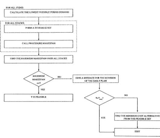
3.1 Flowchart of the Algorithm 31

3.2 Flowchart of the Procedure l''KASiniLITY 33

3.3 Flowchart of the Procedure SCHEDULING... 46

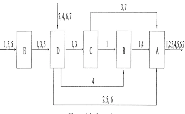
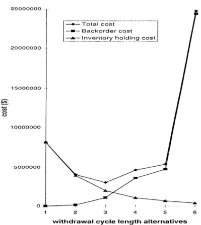
4.1 La.^mut... 51 4.2 The dcta.iled analysis of cost co m p o n e n ts... 54

List of Tables

4.1 Experimental Fa.ctors... 48

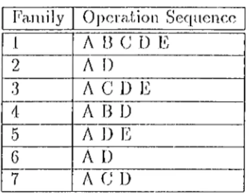
4.2 Family Routing.s... 50

4..3 Comparison of the minimum inventory levels of algorithms . . . 55

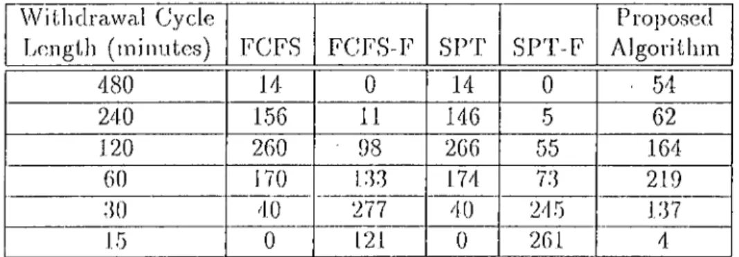
4.4 Comparison of the inventory holding costs of algorithms 56 4.5 Com[)arison of the number of instances of withdiawal cycle lengths of a lg o rith m s... 56

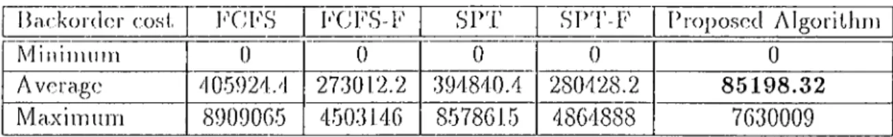
4.6 Comparison of the backorder costs of algorithm s... 57

4.7 Compa.rison of the fdl rates of algorithm s... 57

4.8 Comparison of the tota.l setup tijnes of a lgorith m s... 58

4.9 Comparison of the run times of a lg o rith m s... 58

4.10 F values and Significance Levels (j>) for ANOVA results of th proposed a lg orith m -1 ... 63

4.11 F values and Significance Levels (p) for ANOVA results of the ])roposed algorithm -II... 64 4.12 F values and Significance Levels (p) for ANOVA results of FCFS-I 65

4.13 F values and Significance Levels (|)) for ANOVA results of FCFS-M 66

LIST OF TABLES

Xll

5.1 Data for mimerical example 69

5.2 The period (lcm;riKls for the items 70

5.3 The sequence-dependent setup times (in minutes) 70

A .l The minimum inventory levels for the proposed algorithm . . . . 114

A .2 The minimum inventory levels for F C F S ... 114

A.3 The minimum inventory levels for F C F S - F ...114

A .4 The minimum inventory levels for SPT 114 A .5 The minirnum inventory levels for S P T - F ...115

A .6 The inventory holding costs for the proposed a lg o r ith m .115 A .7 The inventory holding costs for F C F S ... 115

A .8 The inventory holding costs lor FCFS-F ... 115

.9 The inventory holding costs for SPT ... 116

A. 10 The inventoiy holding costs for S P T - F ...116

A. 11 The ba.ckorder costs of the proposed algorith m ...116

A. 12 The backorder costs of FCFS ...116

A. 13 The 117 A. 14 The backorder costs of S P T ...117

A. 15 The backorder costs of S P T - F ... 117

A .16 The fill rates for the proposed a lg o r it h m ... 118

LIST OF TABLES XI и

A .lB T lic fill rates for F C F S -F ... F18 Л.19'Г1)с fill rates for S P T ... FI8

Л.20 The fill rates for SPT-F ... 119

Л.21 'ГЬе total setup tiroes for the proposed algorithm ...119

A .22 The total setup tiroes for F C F S ...119

A .23 The total setup tiroes for F C F S -F ...119

A .24 'The total setup tiroes for S P T ... 120

A . 25 The total setup times for S P T -F ...120

B . l The miuirouin inventory levels for the proposed algorithm . . . . 122

B.2 'I'he inininuiro inventory levels for F C F S ... 122

B.3 The minimum inventory levels for F C F S - F ... 122

B.4 The minimum inventory levels for S P 'F ... 122

B.5 The minimum inventory levels for S P T - F ... 123

13.6 The inventory holding costs for the proposed a lg o r ith m ... 123

B.7 The inventory holding costs for FCFS ... 123

B.8 The inventory holding costs for FCFS-F ... 123

B.9 The inventory holding costs for SPT ...124

B. IO The. inventory holding costs for S P T - F ... 124

B .ll The backorder costs for the proposed a lg o r it h m ... 124

LIST OF TABLES XI V

B.I3 The backoi'dcr costs for b 'C h S -F ... 125

13.14 The backorder costs for З Р 'Г ...125

13.15 The backorder costs for SP4.'-F 125 13.16 The fill rates for the proposed a lg o r it h m ... 126

13.17 The fdl rates for F C F S ...126

13.18 The fdl ratojs for FCk'S-l·^... 126

13.19 The fill rates for Sl’ d ' ... 126

13.20 The fdl rates for SPT-F ... 127

B. 21 The total setup times for the proposed algorithm ... 127

13.22 The total setup times for F C F S ...127

13.2.3 The total setup times for F C F C -F ... 127

13.24 The tota.l setup times for S P T ...128

13.25 The total setui? times for S P T -F ... 128

C . l Performance a.nalysis of proposed algorithm for iirrbala.nced systems ... 130

C.2 Performa.nce analysis of FCFS for imbala.nced s.ystems... 130

C.3 Performance a.nalysis of FCFS-F for imbalanced systems . . . . 130

C.4 Performance analysis of SPT for imbalanced s y s t e m s ... 131

C. 5 Performance analysis of SPT-F for imbalanced s y s t e m s ... 131

LIST OF TABLES X V

D.2 Perfonii<ancc ana.l3^sis of FCFS for S/P r a t i o ... 133

D.3 Pcrformaiico'. a.nalysis of FC[''S- F for S/P r a t i o ... 133

D.4 Performance analysis of SPT for S/P r a t i o ... 134

D. 5 Perforn)a.nce analysis of SP'l'-F for S /P r a t i o ...134

E. l Performance analysis of proposed algorithm for B/1 ratio . . . . 136

E.2 Performance analysis of FCFS for B /I ratio ...136

E.3 Performance analysis of FCFS-F for B /I r a t i o ... 136

E.4 Performance analysis of SPT for B /I r a t i o ... 137

Chapter 1

Introduction

In the last years, the term just-in-time (JIT) has become a common term iii repetitive mamifacturing. It is used to describe a management philosophy that encourages cliange and improvement through inventory reduction. JIT can be defined as the ideal of having the necessary amount of material available

where it is needed and when it is needed. It is a.n attempt to produce

items in the smallest possible quantities, with minimal waste of human and natural resources, and only when they are needed. JIT systems have proven to be effective at meeting production goals in environments with high process relia.bility, low setup times and low demand variability [Groenevelt (1993)].

In general, JIT has a pull system of coordination between sta.ges of production. In a pull system, a production activity at a stage is initiated to replace a part used by the succeeding stage, whereas in a push system, production takes place for future need. The push system is basically a planning system, whereas the pull system is an execution system [Olhager (1995)].

Some of the often cited benefits of JIT production include:

»

• reduced inventories. reduced lead times.

• hi giver qiualil.y,

• rijcluced sera.]) a.ii(l rework ra.l.es, • abilil.y to keep schedules,

• increased flexibility, • easier automation,

• better utilization of workers and equipment.

CH AFTER 1. INTRODUCTION

All of these ultimately translate into reduced costs, higher quality fuiished products, and the ability to compete better. However, there is a limit to the extent that .JIT can be usefully applied in many industries. The major JIT successes a.re in repetitive ma.nufacturing environment. If the demand cannot l)e predicted accurately a.nd product variety ca,nnot be constrained, it is not possible to implement JIT eflectively. J'he final assembly schedule must also be very level and stable. Any major deviations will cause upstream stages to hold larger inventories which will destroy JIT nature of the system. In general, in pull a.]>proaches, information flow is tied to material flow. As a result valuable information (e.g. on the dema.nd trend) is not sent to all stages of production as soon as it is available. Pull systems can therefore be characterized by large information lead times, especially where there are large material flow times.

Justification of JIT implementation ca.n be supported from several angles. Most of the traditional systems (such as material requirements planning (M RP) or reorder point systems) are static systems emphasizing the status quo. In these systems, the emphasis is on achieving individual operation standards, and the aim is to avoid any deviation from the standard. If current values of jnanufacturing variables are met, then the system is regarded as successful. JIT, on the other hand, seeks to change the values of the manufacturing variables. It does this by organizing the production process so that small inventories are strategically placed throughout the process and then carefully reduces these inventories to expose production problems which when solved reduce costs and lead times, and improve quality. JIT uses an enforced problem

solving approaol). Becausoj the inventory is reduced to a. rnininniin, the system raiinot tolera.te any inte.rrnption; tlierefore extreme eaie is taken to find out and solve any production problems. In traditional systems, no such incentive to solve production problems is available.

One of tlie major elements of JIT philosophy and i:>ull mechanism is the Kanl)an system. Kanban is the Japanese word for visual record or card. In Kanban system, cards are used to authorize production or transportation of a given amount of material. This system is the information processing and hence shop floor control system of JIT philosoph3c While kanbans are being used to pull the parts, the}' are also used to visualize and control in-process inventories. The system effectively limits the amount of in-process inventories, and it coordinates production and transportation of consecutive stages of production in assembly-like fashion. Therefore, Kanban system is the manual method of liarmoniously controlling production and inventory quantities within the plant. The Ka.nl)an system appears to be l)cst suited for discrete part production feeding an assembl}^ line.

There are a number of variants of Kanban system. The dual-card

Kanban system employs two types of kanban cards: production kanban and transportation (also called conveyance or withdrawal) kanban. Transportation kanban defines the quantity that the succeeding stage should withdraw from tlie preceding stage. Each card circulates between two stages only; the user stage for the part in question and the stage which produces it. Production kanl)an, on the other hand, defines the quantity of the specific part that the producing stage should manufa.cture in order to replace those which have been removed.

For a Kanban system to operate effectively, very strict discipline is required. This discipline relates to the usage of the kanban cards. There are six rules for dual-card Kanban system on the usage of the kanbans [Browne et al. (1993)]:

CHAPrER 1. INTRODUCTION

3

R u le 1: A stage should withdraw the needed products froni the preceding stage according to information provided on the transportation kanban.

R u le 2: A stage should produce products in quantities withdrawn the succeeding stage according to the inrorma.tion |)iovided by the production I<a.nba.n.

R u le 3: If there is no kanban card, there will be no production and no transj)ortation of parts.

R u le 4: Defective products should never be passed to the succeeding stage. R u le 5: The number of kanbans can be gradually reduced in order to improve the processes and reduce waste.

R u le 6: Kanba.ns should be used to ada.pt to only sma.ll fluctuations in demand.

CHAPTER 1. INTRODUCTION

4

The first three rules tell that parts should be withdrawn and produced ‘just-in-time’ as the.y are needed, not before they are needed and not in larger quantities tha.n needed. Tlie fourth rule causes a rigorous quality control

at each stage of production process. The fifth rule conveys the fact that

inventory can be used as an independent control variable. The level of in- process inventory ca.n be controlled by the number of kanbans and kanban sizes in the system at any time. The sixth rule is related with the limita.tions of tire Kanban system. Kanban system can react effectively only to srna.ll fluctuations in demand. Monden (1984) states that the Kanban system should be able to ada.pt to daily cha.nges in demand within 10 % deviations from the raoiithly master production schedule (MPS).

Kanban system can be either instantaneous or periodic review system. In instantaneous review systems, the kanbans are dispatched upstream as soon as an order occurs. In periodic review systems, the kanbans are collected and dis]ratched periodically. Periodic review sj^stems may be either fixed quantity, nonconstant withdrawal cycle, or fixed withdrawal cycle, nonconstant quantity

[Monden (1981)]. Under the fixed quantity, nonconstant withdrawal cycle

system, kanbans are dispatched upstream when the number of kanbans posted on a withdrawal ka.nban post reaches a predetermined order point. Under the fixed withdrawal cycle, nonconstant quantity system, the period between materia.l handling operations is fixed and the quantity ordered depends on the usa.ge over the withdrawal cycle.

The use of a. Kanba,n system without JIT philosophy makes little sense. The prerc(|uisit(;s of the system (design of the manufa.cttiring system, smoothing of production, standardizcation of ojrerations, etc.) must be implemented before an effective i:>ull system can be implemented. For a. Kanban system to work well, a number of requirements have to be fulfilled. Since each dailj' assembly schedule must be very similar to all other daily schedules, it is essential that it is possilrle to freeze the master production schedule for a fixed time period. The final schedule must be very level and stable. The manufacturing system should conform as closely as possible to the rejietitive manufacturing system. Mixed model capability in all stages of the production process is required to run a mixed model system effectively.

The Kanban system performs best when;

• demand for parts is steady and has sufficient volume, • setup times are small,

• the equipment is reliable, and • defect rates are low.

Cll AFTER 1. INTRODUCTION 5

A Kanban system is ineffective in achieving JIT production for items with low volume; i.e., less than a day’s consumption per container. Since at each stage there is at least some inventory for a product, too much in-process inventory would accumulate for items that require only infrequent production.

Demand fluctuations have a tendency to become amplified from one stage to the next when timing atid size of the replenishment orders are based on locally observed demands as in a pull system [Kimura and Terada (1981)]. Therefore, any major deviations will cause a ripple effect through the production system causing upstream stages to hold larger inventories.

Items with large setup times are more difficult to manage with the Kanban system. Large setup times require large lot sizes, and large lot sizes inflate lead times and in-process inventories. Unreliable systems, i.e. systems with

CHAPrER 1. I N m O D U C r i O N

unreliable rnachines and higli defect rates, cause sijriilar problems. In unreliable systems, the salety factor should be high enough to dea,l with the unexi)ccted events, so the iu-process invcjitories increase. The increase in lead times and in-process inventories destroy .JIT nature of the system.

Even though l.he dua.l-card Kaniran system provides strong control on the production system, due to its strict assumptions and prerequisites, it is clifTicult to implement it. Therefore, a variant of this system, called single-card Kanban system, is sometimes used as a first stage to develop a dual-card Kanban system. In single-card Kanban system, the transportation of materials is still controlled by transportation kanlrans. However, the production ka.nbans to control the production within a cell is absent. Instca.d, a production schedule provided by the central production planning is used. Hence the system ha.s a strong similaiil.y to a conventional push system, with pull elements added to coordina.te the transportation of the |)arts. One of the a.dva.ntages of single­ card push-])ull system is its simplicity in implementation. Moreover, as the information on demand trend is sent to cill stages of ])roduction as soon as its available, single-card Kanban system has shorter informatioji lead times com])ared to dual-card Kanban systems.

In this study, we propose an algorithm to determine the withdra.wa.l cycle length, number of kanbans and kanban sizes of a periodic review Kanban system simultaneously in a multi-item, multi-period, multi-stage ca.pa.citated modified flowline structure production setting with fixed withdrawal cycles. The proposed algorithm considers tlie impact of operational issues, such as

ka.nban schedules and actual lead times, on tlie design parameters. The

production setting is imperfect in which

• demand may be variable,

• setup times may be significant, and • production line ma.y be unbalanced.

CHAPTER

/.

on I,lie limil.a.tions of tire existing models. Chapter 3 is dedicated to problem d('(lnition. After stating l.he motivating points behind this study, the problem is dc'fined, the underlying assumptions are stated, and the pi'oposed algoi ithm is explained. In Cha.))ters 4 and 5, the experimental results are given and a numerical cxa,mple is presented, respectively. Finally, Chapter 6 concludes the study with suggestions for the future research.

Chapter 2

Literature Review

I I I Uiis rhapler, l.lie rclaled lileralurc is reviewed. First, a. review of Ka.nba.ii systems is presented. 'To be able to compaie tlie existing studies, we divide the models into two jjarts; models for determining the design parameters are reviewed in Section 2.1, and tlie models for determining the kanban sequences a.re reviewed in Section 2.2. In Section 2.3, brief reviews on dne-date estimation and group technology a.re given. Section 2.4 summarizes this chapter.

2.1

Determining the Design Parameters

This section reviews the models for determining the design parameters in a. Kanban system. To discuss and compare the models, first a. tabular format is introduced. Then, the models are explained briefly. Fina.lly, the limitations of the existing models a.re sta.ted.

In the tabular format the below characteristics are considered:

1. M o d e l S tru c tu re : Matlicmatical Progra.mming, Simula.tion, Markov Chains, Others

CUA PTER 2. UTERATURE REVIEW

2.1 Heuristic

2.2 Exa.ct: Dynamic Progi irmniing, Integer Programming, Linear Program­ ming, M ixed Integer Programming, Nonlinear Integer Programming.

3. Decision Variables:

3.1 number of kanbans 3.2 order interval 3.3 safety stock level

3.4 ka.nl,ia.n size

4. Performance Measures

4.1 number of kanbans 4.2 utilization

4.3 measures: Inventoi'y holding cost, Sliortage cost. Fill rate 5. O b je c t iv e :

5.1 Minimize cost: Inventory Holding Cost, Operating Costs, Shortage Cost, SeTup Cost.

5.2 Minimize inventory

6. Setting:

6.1 La.yout : Assembly-tree, Serial, Network without ba.cktracking

6.2 Time period: Multi-period, Single-period 6.3 Item: M ulti-item, Single-item

ClfAPTEIl 2. LITERATURE REVIEW 10

6.5 Capacil.y; Capa.cil.atccl, UucapacHated

7. Kanban type: Singlc-ca.rd Ka.nban, Dual-ca.rd Kanban

8. Assumptions:

8.1 Ka.nba.n Sizes: Known, Unit

8.2 Stocliasticity: Demand, Lead time. Processing time 8.3 Witlidrawai Cycle: Fixed witlidrawal cycle, Instanteneous 8.4 No Shortages

8.5 System Reliability: Dynamic demand, Maclune unreliability. Imbalance between stages. Rework

Most of the existing studies in the literature are modeled by using mathematical progra.mming, simula.tion or Markov chains. There are a few exceptional studies that use other methods such as statistical analysis or Toyota formula. In the tabular format, we collect these models under the heading ‘others’ .

For the mathematical formuhations a solution approach should also be stated. This apiiroach can be either heuristic or exact. For exact solution, diilerent methodologies such as dynamic programming, integer programming, linear programming, mixed integer programming, and nonlinear integer prograrnmiug can Ire used.

For the analytical models the decision variables and for the simulation models the performance measures should be indicated. The decision variables are kanban sizes, number of kanbans, withdrawal cycle length for periodic review models, and safety stock levels. The performance measures are number of kanbans, machine utilizations, inventory holding cost, baekorder cost, cind fdl rates. Fill rate can be defined a.s the probability that an order will be satisfied through inventory. Models can consider dilferent combinations of the criteria, stated above.

CHA PTER 2. LITERATURE REVIEW 11

'I'he objeclives for tbc analy(.ic;rl models can be minimizing the costs or minimizing tlie inventories. For tlie cost minimiza.tion, tlie cost terms ca.n be considered eitlier independently as inventory liolding cost, shortage cost, a.nd setup cost, or the comlrination of these costs as operating cost.

The production setting for the models inchide the layout, number of time periods, number of itcuns, number of stages, and the capacity. La,yout can be serial (ilowline), assembly-tree, or a. general network without backtracking (modified flowline). An empty cell in the tables for any of these indicate that the chara.cteristic is not considered in the corresponding study.

Ka.nban system can be either a single-card Kanban system or a dual- card Kanban system, d’hc assum|)tions for the models arc also stated in the ta.bular format. Tlie.se assumptions a.rc the ones that a.re commonly considered, more siiccific ones are indicated in the explanations of the models. The first assumiition is on ka.nban size. An empty cell for this diaracteristic indicates that the kanban size is not a parameter, but is a decision variable for the sj'^stem. Another assumption relates to tfie nature of the system such that the .system can be either stochastic or deterministic. For the deterministic models, this cell is left empty. For the stochastic ones, the stochastic pa.rameters are indicated. The withdrawal cycle lengtli shows if the system is an instantaneous or a periodic review system. The fourth assumption is related with backorders. An empty cell indicates that liackorder is allowed. And, the last assumption is on the system relia.bility. If the system is reliable, this cell is left empty, otherwise the unrelia.bility of the system is stated.

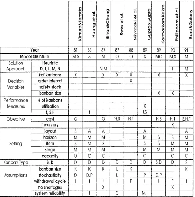
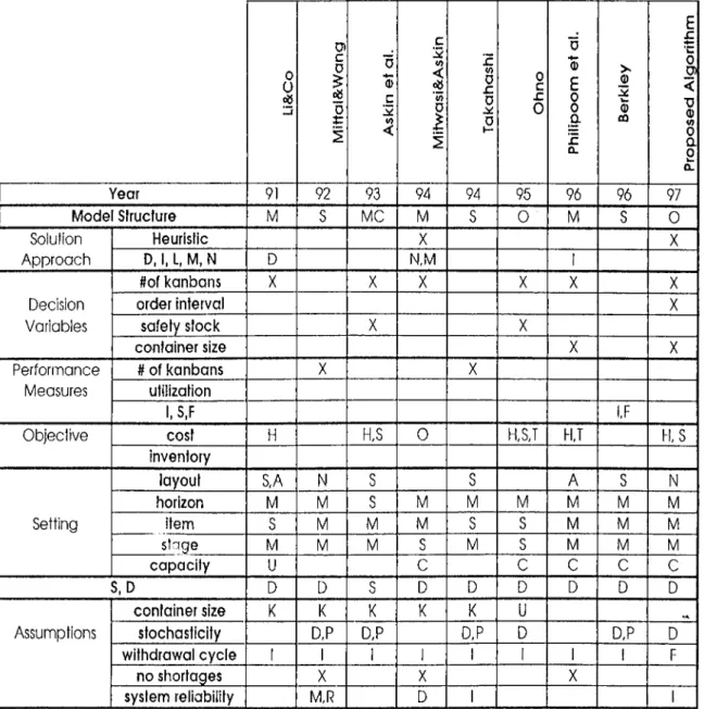
In Figures 2.1 and 2.2, the models a.re presented by using the above scheme. Further explanations of the models are given below:

Kimura and Terada (1981) describe the operation of Kanban systems and examine the accompanying inventory fluctuations in a. .JIT environment. They provide several balance e(|uations for Kanban systems in a. single item, multi­

stage, unca.pacitatecl serial production setting. They use these eciuations

to demonstrate how demand fluctuations of the final product influence the fluctuations of production and the fluctuations of inventory at the upstream

CHAPTER 2. LITERATURE REVIEW

12

O b jec tiv e cost 0 0 H.S H,T H,S H J S,H,T

inventory X Setting layout S A A A A horizon M M M M S s M item s M S S S M M stage M M M M M M M c a p a c ity u C c C c c K anban Type S,D D D D D D D S,D D s Assumptions kan b an size K K K U K K stochasticity D D,P L P D,P w ithdraw al c y c le I 1 1 1 F 1 1 F 1 no shortages X X system reliability 1 D M,l

CHAPTER 2. LITERATURE REVIEW

13

O b jec tiv e cost H H,S 0 H,S,T H,T I t s inventory Setting layout S,A N S S A S N horizon M M S M M M M M M item S M M M S S M M M stage M M M s M S M M M c a p a c ity u c C C c C S .D D D s D D D D D D Assumptions container size K K K K K U stochasticity D,P D,P D,P D D,P D w ithdraw al c y c le 1 1 1 1 1 1 1 1 F no shortages X X X system reliability M,R D 1 1

CUAVTER 2. UrERATUliE REVIEW 14

stages. Tlie a.uthors use sinuilation to show tlia.t fluctuations are amplified when the size of order and/or lead time becomes large.

Huang et al. (1983) simulate the .JIT (by using Q-Gert) with kanban for a multi-line, multi-stage production system in order to determine its a.da.ptal)ility to a. U.S. production environment. The simulated production system includes variable irrocessing times (normally distributed), variable master production schediding (cx])oncntially distributed demand), and imbalances between production stages. The authors conclude that the variability in processing times and demand rates are amplified in a multi-stage setting, and that excess capacity has to Ire available to avoid bottlenecks.

Monden (1984) comments on the conclusion drawn by Huang et al. (1983). He stated that the Kanban system should be able to a.dapt to daily cha.nges in demand within 10 % deviations from the monthly MPS. Larger seasonal fluctuations in deiTiand can Ire a.ccomm(rdated by setting uj) the monthly MPS appropriately.

Bitran a.nd Chang (1987) formidate a. nonlinear integer program to extend Kimura and Terada’s (1981) serial model. 3.'hey provide a. formulation for the Kanban system in a deterministic single item, multi-stage ca.pacitated

a.sscmbly-ti-ee stntcture production setting. Tlie formulation assumes zero

transportation lead time and planning periods of known leiigth and finds the

minimum feasible number of kanba,ns. The authors show that the initial

nonlinear model ca.n be transformed into an integer linear program with

tlie same feasible and optimal solutions. The model does not incorporate

uncerta.inties.

Rees et al. (1987) develop a methodology for dynamicall}'^ adjusting

the number of kanbans in an unstal.)le production environment. They use time series methods and historical data to estimate the autocorrelation and distrilnition functions of lead time. They use To3mta equation witli unit kanban capaciticîs to determine the number of kanbans.

CHAPTER 2. LITERATURE REVIEW

15

(liO Q ) model to detemiine the average inventory for fixed interval witlidrawal and supplier Kanban systems, give formulae to determine the minimum number of kanbans required, and derive an algorithm to ol)ta.in the optimal order

interval. The objective is to minimize the average inventory holding and

ordering costs in a deterministic setting.

Gupta a.nd Gupta. (1989) simula.te (by using System Dynamics) a single item, multi-line, multi-sta.ge, dual-card Ka.nban system. They investigate the impact of changing the number of kanbans and kanban sizes on the performance of the system. The performance measures are chosen to be in-process inventory, capa.city utilization or [)roduction idle time and shortage of the final product. The authors conclude that determining the number of kanbans is essential to the performance of the system, a.nd kee])ing the buffer size consta.nt by increasing the ka.nl)a,n size and decreasing the number of kanl)a.ns accordingly increa.ses tlie inventory. For the smooth operation in a .JIT environment the stages should be l.)alanced and tlie suppliers should be relial)le. And finally, the system performance declines with an increase in demand variability.

Karmarkar and Kekre (1989) develop a continuous time Markov model to study tlie effect of batcli sizing policy on production lead time and on inventory levels. Both single and dual card Kanban cells and two-stage sjestems ai'e modeled. The effect of varying the number of kanbans in the cell is also examined. The primary intent of the investigation is to develop a qualitative a.nalysis of Kanban systems that can provide insights to parametric beha.vior of Kanba.n systems. The results show that the kanban size has a significant effect on the performa.nce of the Ka.nba.n systems.

Pliilipoom et al. (1990) describe the signal kanban technique and

demonstrate two versions of an integer mathematical programming approach for determining the optimal lot sizes to signal kanbans in a multi-item multi­ stage setting. A simulation model is employed to test the efTectiveness of the programming models. The models assume no Irackorders, therefore the sta.ges are decoupled and interdependencies are eliminated.

cm

A PTEIl 2. LITEUATiniE REVIEW

16

determine the number of kanbans at each stage in a multi-item, multi-stage capacitated general assembl,y shop. The objective is to minimize inventory holding, sliortage and setup costs for a given demand and planning horizon without violating the basic kanban principles. They show that the resulting sohd.ions have total costs of approximately half those olrtaiiied using the Toyota equa.tion. Tlie model is most a.ppropria.te when the demand is steady and the leaxl times are short.

Li and Co (1991) develoj) bounds for an eificient kanban assignment and apply them to solve dytiamic programming model in a deterministic, single

item, multi-stage, serial/a.ssembl3^-tree structure production setting. This

model is a.n extension to Bitran a.nd Chang’s (1987) model. The authors assume infinite ca.|)a.city. This assumption not onl^^ removes the capacity constraints but also eliminates the need to keep track of the number of units in partially filled kaulians. Therefore, the model is computationally very efficient, even for a. comirlex non-serial s,ystem.

Mittal and Wang (1992) develo[) a da.ta.base oriented simulator, CADOK (Computer Aided Determination of Kanbans) to determine the number of kanbans in a production setting where breakdowns, reworks, setup times, variable processing times (normally distributed), and variable demand (exponentially distributed) are modeled. Backorder costs are assumed to be prohibitively high. The model ca.n handle both assembly and disassembly type opera.tions, that is to sa.y, several sta,ges supply products to the same sta.ge and one sta.ge supplies parts to several stages, respectively. Also, dela.y can

be induced for the information to l.ravel from one stage to another. But,

the system cannot handle backtra.cking so it is only applicable to flowlines or modified flowlines.

Askin et al. (1993) develop a continuous time, steady-state Markov

model for determining the optimal number of production kanbans in a multi­ item, multi-sta.ge serial production .setting. The objective is to minimize the inventory holding and sliortage costs given external demand and the kanban sizes. The external demand assum|)tion permits the modeling of a multi-stage

CHAPTER 2. LITERATURE REVIEW

17

system as inclepencleut sta.gcis. The model uses Toyota, equation and finds tlie numher of kanlia.ns a.iid sa.rel.y la-ctor. The |)el·Γoı■ma.nee of tlie model is sensitive to the a.ecura.te estimation of the (|ueue lengths.

Mitvvasi and Askin (1994) ])i;ovide a nonlinear integer matliematical model for the multi-item, single stage, capacitated Kanban system. It is assumed that demand is external, dynamic and evenly distributed over ]:>eriod, the system is reliable, setups are small enough to allow batch sizes as small a.s a single kanban, and no shortages are permissible. The control periods are assumed to be small enough to ignore batch sequencing problem. The model is transformed to a simpler model with the same set of optima.! and feasible kanban solutions. Lower and upper bounds for number of ka.nba.ns a.re develoj)ed. A heuristic solution is a.lso presented.

Taka.ha.shi (1994) provides a. simulation model to determine the number of ka.nba.ns for single item, unbalanced serial production systems under stochastic conditions (demand with exponential distribution and processing time with ga.rama. distribution). An algorithm that allows different numbers of production and withdrawal kanbans at an inventory point is proposed. It is assumed that the total nund:)er of kanbans are known, withdrawal lead time is negligible, and backorders are allowed.

Olmo et al. (1995) derive the stability condition of a JIT production system with tlie production and supplier kanbans under the stochastic demand and

deterministic processing times. An algorithm for determining the optimal

number of two kinds of kanbans that minimize an expected a.vera.gc cost per period is devi.sed. In other words, this algorithm determines the optimal safety stocks in 'I.'oyota (xjua.tion.

Philipoom et al. (1996) provide a nonlinear integer mathematical model for the multi-item, multi-stage, multi-period, capacitated Kanban system. It is assumed that demand is deterministic, the system is reliable, setups are sequence-independent, production costs are stable, lot sizes remain constant throughout the shop and no shortago^s are permissible. The model determines kanban sizes, number of kanbans, and final assembly sequence simultaneously

CUAFTER 2. UrERyVrURE REVIEW

18

by minimizing Ihe setup and inventory bolding eost.

Ilerkbiy (I9!)(i) investiga.t('s tlu' eflert of kiutba.ii sizc^ on systi'in peiTonna.nc('-

in a multi-item, multi-stage, dual-card Kanban system. The performance

measures are in-]:)rocess inventory and customer service level. The author varies the numl)er of ka.nbans and kanban sizes in the tandem so that the total in-process inventory ca.pa.city remaijis constant. Simulation results show that smaller kanban sizes lea.d to sma.ller in-process inventoricis, and srna.ller ka.nba.n sizes can lea.d to better customer service when the cost of the greater setup times ca.n l)e offset l)y the Ijcneiits of more fre([ucnt material handling. 7'he study assumes that the kanban sizes and number of kanba.ns are same for a.ll pa.)'ts and the set of kanlran size values are independent of the demand distribution.

The limitations of the a.na.lytical models can be stated as follows:

• Most of the models assume that the kanl)a.n sizes are known. The

except,ions are Gupta, and Gupta (1989), Karmarkar a.nd Kekre (1989), and Philipoorn et al. (1996). In the remaining studies, it is a.ssumed that kanl)a.n sizes are known a.nd the number of kanbans are determined by using these predetermined values. In fact, number of kanba.ns and kanban sizes should be determined simultaneously, as these two together affect the i)erforma,nce of the system. It is not known under what conditions large ka.nban sizes and small numbers of kanbans are [)referred to small kanba.n sizes with large numbers of kanbans.

• Almost none of the models, except Philipoom et a.l. (1996), consider the impa.ct of operating issues on design parameters. For example, it is usually assumed that the control periods are small enough to ignore batch seciuencing problem. Even in the study of Philipoom et ah, only the final assembly sequence is determined and it is assumed that it propa.ga.tes back by the first-come-first-served (FGFS) rule.

• In general, instantaneous mateiial handling is used. There are only two models that use noninstantaneous material handling, liy Miyazaki et al.

CHAPTER 2. LITERATURE REVIEW

19

(1988) ami Pliilipoom cl. al. (1990). Pliilipooin et al. (1990) develop a model for signal kanbans, a.nd Mi_ya,zaki et al. (1988) develop a model for supplier and withdrawal ka.nba.ns. The model structures are different, and tlie findings cannot be generalized to a dual-ca.rd Kanban s,ystem. • Several models assume station independence. Askin et al. (1993) and

Mitwa.si and Askin (1994) assume externa.l demand. The demand for each sta.ge is externally generated and with the a.ssumption of sufficient capacity, the multistage system ca.n be modeled as independent stages linked by their proportional demand rates. Bitran and Cha.ng (1987),

Philipoom et al. (1990) and Philipoom et al. (1996) do not allow

ba.ckordcrs. Under .IIT system, all stages are integrally tied to each

otlier and if one dela.ys a.ll the otliers may be affected. But, with the a.ssumi)tion of no backorders, this possibility is eliminated. Therefore, each stage can be modeled indei)endently.

• Kimuraand Tera.da (1981), Philii)oom et al. (1990), and Li and Co (1991) assume tha.t the ca,pa.city is unlimited. In that wa.y, tlie formulation of the model becomes easier.

Tlie limitations of the simulation models can be stated as follows:

• Even though simulation olTers a number of advantages by restricting the number of a.ssumptions of the system, it takes a grea.t deal of time

to develop simulation programs. Ai)art from reaching at optimality,

one must test many alterna.tive shop configurations. Almost all of the simulation models assume demand to be exponentially distributed. More realistic assumptions on the demand distribution are necessary.

• Simulation studies to determine the interaction of kanban sizes and number of ka,nba.ns are needed. Berkley (1996) study the effect of kanban sizes on system performance, but he assumes that the kanban sizes are set regardless of the demand distribution. Studies with more general assumptions on determination of the kanban sizes should be performed.

CHAPTER 2. LITERATURE REVIEW

20

2.2

Determining the Kanban Sequences

In JIT systems, the final assembly schedule determines production schedules for all of the stages in tire facility. Once the assembly line is scheduled, it is assumed that the sequence propagates back through the system. Kanbans in the rest of the shojr are processed in order in which tho,\y are received, i.e. (FCFS). However, there are several studies in the literature tha.t test this assumption.

Lee (1987) compares FCFS, shortest processing time (SPT), SPT/LATE, higher pull demand (HPF), and IIPF/LATE in a flow shop using dual-card Kanban system with .fixed order points. Simulation results show that SPT and SPT/LA 'l'E out[)erform in several ])crformance measures considered such as irroduction rate, utilization, (pieue time, and ta.rdinc:ss. 'I.'he same system is simida.t(xl l,o s<h' tlu'. (dlect of difleixuit job mixes, pull ra.(,es, and number of kanbans and kanban sizes on the system performance.

Berkley and Kiran (1991) compare the performance ' of SPT, FCFS, SP'I'/LATE, and FCFS/SPT in a dual-card Kanban system with constant withdrawal cycles. They find that contrary to the conventional results, SPT creates the hugest a.verage output material queues and in process-inventories, and FCFS and FCFS/SPT creates l.he least. FCFS and FC FS/SPT outperform otliei' two rules.

Berkley (1993) compares the performance of FCFS a.nd SPT in a single- card Kanljan system with varying queue capa.cities a.nd mateiial handling frcqucncic's by a simuhition model. J'he residts of the study arc compa.red with the results of Berkley and Kiran (1991). It is shown tha.t the results are due to material handling mechanism used in both of the models.

Liimmus (1995) simulates a JIT system to investigate the effect of sequencing on tlie performance of the system in a multi-item, multi-sta.ge assembly-tree structure setting. The author use three sequencing rules, which are Toyota’s goal chasing algorithm (a detailed explanation of the algorithm can be found in Monden(1981)), demand-driven production and producing all

CIIAFTER 2. LITERATURE REVIEW

21

the jobs of the same kind, and stud_y their effects for different sequences given various setuj) a.nd ])rocessing times. .She concludes that the sequencing method .selected affects tlie performa.nce of the system.

The problem of production leveling through scheduling is crucial to Ka.nba.n

systems. Sequencing in kanban-controlled sliops are more complex when

compared to conventional sequencing problems a.s kanbans do not ha.ve due da.tes and ka.nban-controlled shops have station Irlocking [Berkley(l992)]. Sta.tion blocking ca.n be described as the idleness of a stage due to full outbound

inventories. Although there are several studies on kanban scheduling, the

rules used in these studies are simple dispatching rules. More sophisticated scheduling rules should be used to determine the effects of scheduling on the performance of the system.

Detailed reviews of .JIT and Kanban systems can be found in Berkley (1992), Groenevelt (199-3), a.nd Ilua.ng and Kusia.k (1996).

2.3

Related Literature

To avoid ambiguity throughout the study, we will give brief reviews of due date estimation models and group technology.

2.3.1 Due Date Estimation

Due dates are treated in two ways in the literature; the}' are either externally imposed or internally set. For the internally set due dates, a flow time is estimated for each job and a due date is set accordingly. There are several models in tlie literature for due date estimation in job shop or flowlines. In this section, we will briefly review the work of Ragatz and Mabert (1984). The authors compare eight different due date estimation rules in a job shop setting on a simulation study. They find out that both job characteristics and shop status information should be used to develop due date assignment rules.

G77/\

22

liiformation about workcentcr congestion along tlic routing of a job is more useful than the general shop information. Moreover, the use of more detailed information in predicting flow times provides only maxginal improvement in performa.nce over other rules that use more aggregate information.

More detailed armJysis on due date estimation can be found in Vig and Dooley (1993), Russell and Philipoorn(1991) and Mahmoodi et al. (1990).

2.3.2

Group Technology

One of tlie key elements of JIT is group technology (G T). GT is a maiuifa.cturing ])hilosophy that exploits similarities in ])roduct design and

production process. With the application of GT, a wide range of benefits

ca.n be possible, including variety reduction, reduced setup times, lead time and in-])rocess inventory. GT provides the flexibility that support the design and implementation of JIT. JIT includes a simplified production line and standardized products. GT can be used to form families and machine cells which would lead to standardized products a.nd a simplified production line. A family is a group of parts that share the same setup, processing, routing, a.nd so on.

When parts are classified into a families, family scheduling is applica­ ble. A family scin duling procedure incorporates information about family membership and generates solutions which build on the elimination of setups

l)y combining jobs from the same families. There are several studies

on la.mily sclieduling. In our study, we use the findings of Wemrnerlov

and Vakharia (1991). The authors compare four family-based scheduling

])rocedures with four corresponding item-based scheduling procedures on a

flowline manufacturing cell. They find that first-come-first-served-fainily

(FGFS-F) is the best performer among the eight rules investigated. The

authors conclude that for tlie conditions used in the study, family-based scheduling approaches can generate significant improvements with respect to flow timca.nd lateness-oriented measures. Moreover, when setn]) times increase.

CHAP'I’FM. 2. UTERATWIE REVIEW

23

Uic aclva.nta.ge in using fa.mily-ljased rules over iiern-based rules increases.

Del,ailed reviews on GT can Ire found in OfTodile el, al. (1994) and

Guna.seka.ian el, al. (1994). Review on GT scheduling ca.n be found in

VVeınmerlöv a.nd Vakharia. (1991) and Russell and Philipoorn (1991).

2.4

Summary

In this cha.pter, the literature on Ka,nban systems is reviewed. First, the models on determining the design parameters are ex|)lained briefly witli emphasis on their limitations. A tabula.r format is used to compa.re the models. Then, the models for sefjuencing the ka.nl)a.ns are introduced. The results of these studies can be summa.rized as follows:

• In the existing literature most of the studies determine the kanban sizes and number of k'a.nba.ns sepa.ra.tely. In lact, number of kanbans required depends on kanban sizes a,nd these parameters together affect the system performa.nce. Therefore these pa.rameters should be set simultaneously, not sequentially.

• None of the studies consider the impact of operationa.1 issues on design para.meters. The secpiencing in Kanban systems need more elaboration. • Even though dua.l-ca,rd Kanban systems are periodic, in nature, there are

a. limited number of studies on periodic review systems.

In the next cliapter, an algorithm is proposed to eliminate the above cited

limitations of the existing models. The proposed algorithm determines

withdrawal cycle length, kanban sizes, and number of kanbans simultaneously in a periodic review Kanban system. It provides a feedback mechanism to evaluate the impact of operational issues such as scheduling and actual lead times on the design parameters.

Chapter 3

Problem Statement

ill iliis sl.iK.ly, we i)roposc an aiui.lyl.ical model to dctcnniiic the withdrawal cycle length, kanban sizes a.nd number of kanbans simultaneously in a periodic review Kanban system under imperfect production settings. With the proposed algorithm, we try to eliminate the dellciencies of Kanban system due to its strict a.ssuniptions and prerequisites by incorporating flexibility to the system design. We use the impact of operating issues such as scheduling and actual load times on the design parameters. Moreover, we analytically study the effects of system parameters on system performa.nce.

The rest of this chapter is organized as follows: In Section 3.1 the problem is definecl, the motiva.l,ing points are highlighted, and the underlying assumptions are explained. In Section 3.2 the proposed algorithm is discussed. First, the notation used is introduced in Section 3.2.f, then the algorithm is explained in deta.il. The clurpter iinishes with the. concluding remarks.

CUIAPTER 3. PROBLEM STATEMENT

25

3.1

Problem Definition

In iJiis study, an analytical model is proposed to determine the fixed withdrawal cycle length, number of kanbans and kanban sizes simultaneously in a multi­ item, multi-stage, multi-horizon periodic review Kanban system on a minimum cost

The motivating points behind tins study arc as follows:

Even though setting the kanban sizes is one of the primary decisions that tlie designers of a Kanban system must address [Oerkley( 199G)], there are only a limited number of studies that determine the number of kanbans and kanban sizes simultaneously. The recent research has shown that there is a significant relationship between kanban sizes and production lead times, and therefore the shop congestion [Ka.rmarka.r a.nd K ekrc(f989)]. The existing studies reflect the relation among tire ka.iiban sizes and the average inventory, but for the other performa.nce measures no clear rcla.tions a.re present. One of the purposes of this study is to investigate ana.lytically the effect of the kanban sizes on the system performa.nce by using several performance measures such as average in-process inventory, total backorder cost, fill rate and total setup time.

Almost none of the models consider sequencing and determining the design parameters simultaneously. It is generally assumed that once the number of ka.nbans a.re determined, FCFS can be used to schedule the jobs. In fact, tlie ]>iobIcm of production leveling through scheduling is crucial in Kanban systems. Selecting the proper scheduling rules becomes even more important in the case of imperfect production settings, i.e. settings with high setup times, high product variety, and etc. [Huang and Kusiak(I99C)]. In this study, we consider the impa.ct of operating pa.rameters on design parameters.

There are a limited number of studies on periodic review systems. In fact, the review frequency is an important factor in determining the operating parameters, as there is a trade-off between inventory holding cost and setup cost. This trade-off should be reflected in the design of a Kanban system.

CHAPTER 3. PROBLEM STATEMENT

26

In the design of tins proposed algoritlun, we consider severa.1 points to increase the ilcxil)ility and adaptahility of the Kanban systems. Wc aJlocate different nnmber of kanba.ns at each inventory [)oint to decrease the possibility of Idocking and backlogs. We use the idea of transfer Iratch and process batch. In that wa.y, the ka.nban sizes can l)c decreased to low levels and the setup times can l)e jnstified [Browne(1993)]. We estimate the lead times for each stage in terms of periods so tha.t the a.ccnia,cy of the estima.tion increases and the problems due to lead time estimation are minimized. We determine the Kanban sizes according to demand distributions so that the amount of remnants can be decrea,sed.

The following assumptions a.re made through out the study:

• 'I'lie system is a. periodic review system. • Demand is discrete and stochastic.

• The processing times and setup times are deterministic.

• Kanban processing times are equal to the time required to process all pa.rts in a kanban. Half full kanbans are not allowed.

• The setups are sequence dependent. A major setup is required when the family being processed at a stage changes. Minor setups are assumed to be zero.

• All the parts in a family follow the same routing on a modified flowline. Modified flowline is similar to flowline in tliat the material flow is unidirectional, but contrary to flowlines, in modified flowlines stage skippings are allowed.

• The withdra.wa.l lead time is zero.

• Backorder is allowed, but the backorder costs arc higher when compared to inventory holding costs.

• The system is reliable, i.e. there are no machine breakdowns. Processing at each stage is carried out without defects.

CHAPrER 3. PROBLEM STATEMENT

27

• Tlie bill of materials quantity is assumed to be one for caeh component.

Under these assumptions, the withdrawal cycle length, kiinban sizes and nnmbcr of ka.nbans are fonnd. The |ra.rametcrs are as follows:

1. Costs terms:

i. unit inventory holding cost

ii. unit backorder (unmet dema.nd) cost 2. family routings

3. processing times

4. sequence dependent setu]) times 5. demand distributions

The ])roposed algorithm generates several alternatives for withdrawal cycle length and kanban sizes, and chooses the best combination among these by comparing the total inventory holding and backorder costs of each alternative.

To determine the maximum inventory level Toyota formula is used. In Toyota formula, the maximum inventory level is calculated by using the expression,

maximum inventory level = na = DL{1 + s)

where,

n

a is the kanban size,

D is demand,

L is lead time, and

CIIAPTEll 3. PIIOBLEM STATEMENT

28

An ivnporia.nl, ivroljlcin that arise wiili the Toyota fonnulais the estimation of the lea.cl times. Lea.cl time is not an attribute of the part, rather it is a pro])erty of the shop floor. Lead times vary greatly depending on ca,]vacity, shop loa.d, product mix and batch sixes. [Karmarka.r (1987), Karmarkar (1993) and Karmarkar et al. (1985)]. Second, it is shown in Karmarkar and Kekre (1989) tliat tlie number of kaid^ans a.nd kanban sizes have a significant efiect

on the performance of the Kanba,n system. So, it is not possible to think L

independent of these two variables. Therefore, the problem becomes a clifRcult one to solve.

VVe try to climiiurtc the first problem through lead time estimation. We estimate the flow times for each stage by using the ex]vected period demand. There are several studies in the literature for flow time estimation, but they are not directly applicable to our system because of its periodic nature. Therefore, we modify the work-in-queue (W fQ ) rule which is indicated by Ragatz and Mabert (1984) as one of the most promising rules of the due date estimation literature.

For the second problem, various combinations of n and a are tried, and

their eifect on the system is investigated through cost terms.

3.2

The Proposed Algorithm

3.2.1

Notation

The following notation is used throughout the thesis.

I number of lamilies

i family index, i = /

j item index, j = 1,.., size]!]

M : number of sta.ges

CHAPTER 3. PROBLEM STATEMENT

29

withdrawal cycle length

period index, I = 1 , {nop ■ 11)

the set of alternatives of kanban size for item j of family г

for the withdrawa.1 cycle length of 7"

kanban size for item j of family i for withdrawal cycle length T

the set of number of ba.ckorders of items in period I. at stage m

the number of backorders of item j of family i in period t at stage ??г,

i.e. {i, j)ih component of

unit backorder cost of item j of family i at stage m

demand for item .; of family i a.t period I.

(in terms of number of kaul)ans)

dema.nd for item j of family i at period i at stage m

updated demand for ite m ; of family i at stage m

expected flowtimeof item j of family i at stage m

the remnants of item j of family i at period t

planning horizon

unit inventory holding cost of item j of family i at stage rn

the set of in-process inventories of items at the beginning of period t

at stage m

the in-process inventories of item j of family i at the beginning of

period i at stage rn, i.e {i,j)th component of

index set a.t sl.age in at |)criod I,

lead time estimation consta.nt for stage rn

the maximum inventory level of item j of family i at stage rn

number of kanbans for item у of family i at stage m for

withdrawal cycle length T' number of periods per shift

the set of possible withdrawal cycle lengths