T.C.
ISTANBUL AREL UNIVERSITY
INSTITUTE OF SCIENCES
ELECTRICAL-ELECTRONICS ENGINEERING
ANALYSIS OF GAIN AND NOISE FIGURE IN
DIFFERENT CONFIGURATIONS OF EDFA
MASTER OF SCIENCE
YEMİN METNİ
Yüksek Lisans tezi olarak sunduğum “Analysis of Gain and Noise Figure in Different Configurations of EDFA” başlıklı bu çalışmanın, bilimsel ahlak ve geleneklere uygun şekilde tarafımdan yazıldığını, yararlandığım eserlerin tamamının kaynaklarda gösterildiğini ve çalışmanın içinde kullandıkları her yerde bunlara atıf yapıldığını belirtir ve bunu onurumla doğrularım.
ONAY
Tezimin kağıt ve elektronik kopyalarının İstanbul Arel Üniversitesi Fen Bilimleri Enstitüsü arşivlerinde aşağıda belirttiğim koşullarda saklanmasına izin verdiğimi onaylarım:
Tezimin tamamı her yerden erişime açılabilir.
I ÖZET
Bu çalışmada, Erbiyum Katkılı Fiber Yükselteçlerde (EDFA) kullanılan pompalama sinyalinin (1480 nm) yönünün sistemden elde edilen kazancın ve oluşan gürültü faktörünün üzerindeki etkisi incelenmiştir.
Bu tezde 5 bölüm bulunmaktadır. Bölüm-1’de fiberlerin ve optik haberleşmenin tarihçesine kısa bir bakış yapılmıştır. Bölüm-2’de Optik Haberleşme sistemlerinin genel yapısı, kullanılan cihaz ve malzemeler anlatılmıştır. Özellikle SDH sisteminin ve EDFA’nın kullanım alanı olan WDM sisteminin çalışma prensipleri, data kapasitesi, çalıştığı band aralığı anlatılmıştır. Bölüm-3’de EDFA sisteminin matematiksel teorisi anlatılmıştır. İlk kısımda EDFA’nın üç seviyeli temel denklem oranı, iki seviyeli temel denklem oranı, kesişim (overlap) faktörü, ömür zamanı (lifetimes), bant genişliği ve kendiliğinden yükseltilmiş emisyon (ASE) anlatılmıştır. İkinci kısımda EDFA sistemlerindeki kazanç, kazancın fiber uzunluğu ile değişimi, gürültü ve kaskat EDFA anlatılmıştır. Bölüm-4’de bu teze özgün olarak anlatılan yeni önerilmiş EDFA konfigürasyonlarının çözümleri MATLAB programı kullanılarak nümerik olarak incelenmiş olup, elde edilen sonuçlar karşılaştırmalı olarak yorumlanmıştır. Bölüm-5 ise sonuç kısmını içermektedir.
Elde edilen sonuçlardan görülmüştür ki, 1480 nm dalgaboyunda ileri, geri ve iki yönlü olarak pompalanmış tek geçişli ikili katmanlı ve çift geçişli tek katmanlı EDFA konfigürasyonlarında simüle edilmiş, pompalama yönünün gürültü faktörüne, sinyal kazancına ve gücüne olan etkisi incelenmiştir. Sonuç olarak, ileri-ileri pompalama yönlü çift geçişli tek katmanlı EDFA konfigürasyonunda yapılan pompalamanın daha yüksek çıkış sinyal gücü ve kazancı verdiği ve iki yönlü pompalamanın gürültü seviyesinin diğer önerilen pompalama konfigürasyonlarına göre daha düşük olduğu görülmüştür.
II ABSTRACT
In this study our main objective is to design new EDFA configurations to obtain higher gain and lower NF values using an input signal -35 dBm at the wavelength of 1550 nm and the pump power 14 mW at the wavelength of 1480 nm. Utilizing Giles and Desurvire model, we proposed miscellaneous SP and DP EDFA configurations different in the means of pump signal direction where the two level system model equations are solved numerically in Matlab. The physical properties of the simulated EDFA configurations such as gain, noise factor, population density and amplified spontaneous emission were studied under various pumping directions.
III
ACKNOWLEDGEMENTS
I would like to express my deepest gratitude and respect to my supervisor Assist. Prof. Dr. Ufuk Paralı for his excellent guidance, support and constant encouragement throughout my research and thesis.
I would like to say thank you to my wife Çağla, for her encouragements, all her support during my MSc. without whom I wouldn’t be writing these lines.
IV CONTENTS ÖZET---I ABSTRACT---II ACKNOWLEDGEMENTS---III LIST OF ABBREVIATIONS---VII LIST OF TABLE---X LIST OF FIGURE---XI LIST OF APPENDIX---XIV CHAPTER-1
A BRIEF HISTORY OF OPTICAL COMMUNICATION
1.1 Optical Fiber History---1
CHAPTER-2 OPTICAL COMMUNICATION 2.1 Introduction---3
2.2 Optical Communication Theory and Devices---3
2.2.1 Optical Source---4
2.2.1.1 Light-Emitting Diodes (LEDs)---4
2.2.1.2 Lasers---4
2.2.2 Optical Detectors---5
2.2.2.1 Photoconductors---5
2.2.2.2 Photodiodes---6
2.2.2.3 Phototransistors---6
2.2.3 Optical Communication Systems---7
2.2.3.1 Fibre Distributed Data Interface (FDDI)---7
2.2.3.2 SONET and SDH---7
2.2.3.3 Wavelength Division Multiplexing (WDM)---9
2.2.3.4 Free Space Optics (FSO)---12
2.2.4 Optical Passive Conponents---12
2.2.4.1 Fiber---12
2.2.4.2 Couplers---13
2.2.4.3 Isolators and Circulators---14
V CHAPTER-3
ERBIUM DOPED FIBER AMPLIFIERS
3.1 Introduction---16
3.2 EDFA Basics---17
3.2.1 Three-Level System For EDFAs---17
3.2.2 The Overlap Factor and Aeff---20
3.2.3 Lifetimes---21
3.2.4 Linewidths and Broadening---22
3.2.5 Two-Level System for EDFAs---23
3.2.6 Amplified Spontaneous Emission---26
3.3 Modelling and Complex Effects---27
3.3.1 Gain for EDFA---27
3.3.2 Gain as Function of Fiber Length---29
3.3.3 Noise in EDFA---30
3.4.4 EDFA Cascade---35
CHAPTER-4 4.1 Introduction---36
4.2 Single Pass Edfa Configurations---37
4.2.1 Setup, Formulation and Results for Configuration-1 (Forward-Forward Pump)---38
4.2.2 Setup, Formulation and Results for Configuration-2 (Forward-Backward Pump)---43
4.2.3 Setup, Formulation and Results for Configuration-3 (Backward-Backward Pump)---47
4.2.4 Setup, Formulation and Results for Configuration-4 (Backward-Forward Pump)---50
4.3 Double Pass Edfa Configurations---54
4.3.1 Setup, Formulation and Results for Configuration-5 (Forward Pump)---54
4.3.2 Setup, Formulation and Results for Configuration-6 (Forward-Forward Pump)---59
VI
4.3.3 Setup, Formulation and Results for Configuration-7 (Backward
Pump)---63 CHAPTER-5 5.1 Conclusion---68 REFERENCES---70 APPENDIX---83 RESUME---131
VII
LIST OF ABBREVIATIONS
EDFA : Erbium doped fiber amplifier SDH : Synchronous Digital Hierarchy PDH : Plesiochronous Digital Hierarchy SONET : Synchronous Optical Network WDM : Wavelength Division Multiplexing DWDM : Dense Wavelength Division Multiplexing
ETSI : European Telecommunications Standards Institute VC : Virtual Container
TU : Tributary Unit
TUG : Tributary Unit Group
C : Container
AU : Administrative Unit AUG : Administrative Unit Group STM: : Synchronous Transport Module STS : Synchronous Transport Signal
: The spontaneous emission factor
: The optical bandwidth in the frequency domain over which the ASE power is being measured
: The signal input power
: Pump power : Signal power
: Backward signal power : Forward signal power : Backward pump power : Forward pump power IP : Internet Protocol G : Gain of the amplifier ̃ : Noise figure
NF : Noise figure
VIII : Signal Over-lap factor : Pump Over-lap factor
: The transition probability from level 2 to level : The transition probability from level 3 to level 2
: Emission cross-sections : Absorption cross-sections : Pump cross-section : Signal cross-section
: Signal absorption cross section
: Signal emission cross section
: Pump absorption cross section
: Pump emission cross section : Inverted gain coefficient
: Small signal absorption coefficient : Small signal absorption coefficient : Small pump absorption coefficient : Pump flux
: Signal flux
: The populations of level 1 : The populations of level 2 : The populations of level 3 N : The total population density
: The lifetime of level 2 : Total lifetime
: The non-radiative lifetime
ρ : Erbium ion density per unit volume
R : Pumping rate
: Fiber effective area
IX
ASE : Amplified spontaneous emission NF : Noise Figure
h : Planck constant
v : Frequency
: Bandwidth
SNR : Signal-to-noise ratio
OSNR : The optical signal-to-noise ratio
L : Length
g( ) : The gain coefficient : Three level Erbium ion
: Metastable state (level 2 transition) : Ground state (level 1 transition) : Level 3 transition
: Several signals : Several pump : Signal frequency : Pump frequency
: ion density per unit volume : Percent of the reflected signal
C : Circulator
: Up stimulated transition rates : Down stimulated transition rates
X
LIST OF TABLE
Table 2.1 VC Types and capacity (ITU-T G.707/Y.1322 (01/2007))---8
Table 2.2 SDH hierarchical bit rates (ITU-T G.707/Y.1322 (01/2007)) ---9
Table 2.3 Transmission windows used in optical fibers---11
Table 4.1 Parameters of the Single Pass EDFA---37
Table 4.2 SP EDFA results for the proposed configurations---53
Table 4.3 Parameters of the DP EDFA---54
XI
LIST OF FIGURE
Figure 2.1 Optical Transmission---3
Figure 2.2 Stimulated emission in a two level atom---5
Figure 2.3 Photoconductive Detector-Principle ---6
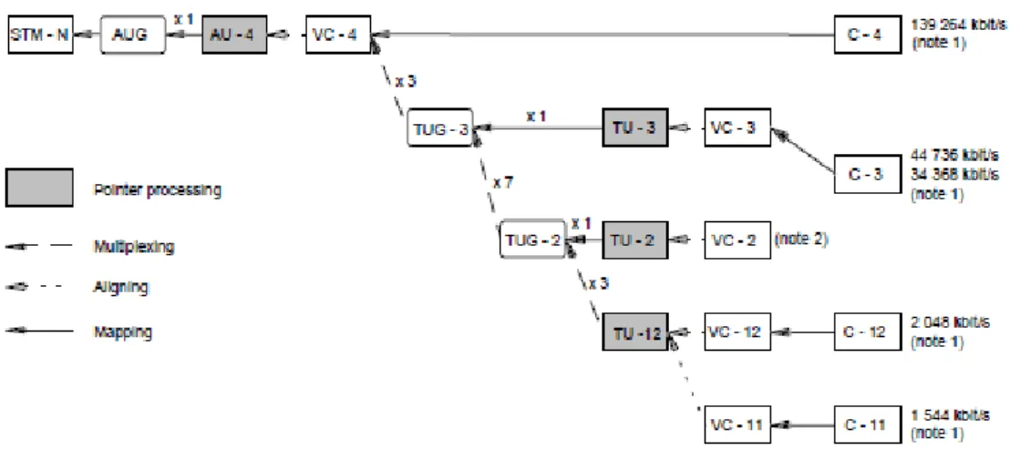
Figure 2.4 SDH multiplexing structure as defined by the European Telecommunications Standards Institute where VC-Virtual Container,TU-Tributary Unit,TUG-Container,TU-Tributary Unit Group,C-Container,AU-Administrative Unit,AUG-Administrative Unit Group,STM-Synchronous Transport Module--8
Figure 2.5 Block diagram of a DWDM system---10
Figure 2.6 Schematic of a step index optical fibre---12
Figure 2.7 Optical Couplers---13
Figure 2.8 Isolator and Circulator---14
Figure 2.9 Filter---15
Figure 3.1 Simplified three level energy diagram of Er3+ for the amplifier model. The transition rates between levels 1-3 and 1-2 are proportional to the populations in those levels and to the product of the pump flux - pump cross-section and signal flux - signal cross-section , respectively. The spontaneous transition rates of the ion (including radiative and nonradiative contributions) are given by and ---17
Figure 3.2 Example of a radial distribution of the erbium ion density in a single-mode fiber and the equivalent “flat top” distribution, which has a constant ion density N stretching from r=0 to r=R ---21
Figure 3.3 Broadening---23
Figure 3.4 EDFA gain performance as a function of the input signal powers in dBm, at wavelength 1549.2 nm, at saturation for pump powers of 40, 65, 100 mW---28
Figure 3.5 Curves of gain G versus pump power ---28
Figure 3.6 Signal gain at 1530 nm (left) and 1550 nm (right) for 1480 and 980 nm pumping of erbium-doped Al-Ge silica fiber, as a function of fiber amplifier length. The launched pump power is 40 mW and the launched signal power is -40 dBm---29
XII
Figure 3.7 Signal gain at 1530 nm (left) and 1550 nm (right) for 1480 nm and 980 nm pumping of erbium-doped Al-Ge silica fiber, as a function of fiber amplifier length. The launched pump power is 10 mW and the launched signal
power is -40 dBm. From numerical simulations---30
Figure 3.8 An EDFA amplifies an input signal, and along with the amplified signal there is a background ASE that constitutes the noise of the amplifier. Any ASE not coincident with the signal wavelength can be filtered using an optical filter. However, ASE within the signal band cannot be filtered and constitutes the minimum noise added by the amplifier---31
Figure 3.9 (a) noise figure and (b) amplifier gain as a function of the length for several pumping levels---33
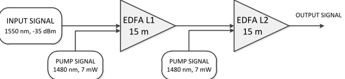
Figure 4.1 Configuration 1: Forward – Forward pump scheme for double stage SP EDFA---38
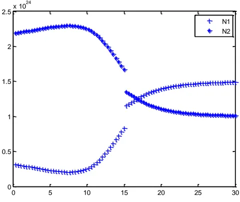
Figure 4.2 Population Density of Configuration-1---40
Figure 4.3 The signal gain as a function of EDFA length with 1550 nm input signal and 7mW pump signals applied at z=0 and z=15 m in configuration-1-41 Figure 4.4 Noise Figure of configuration-1---42
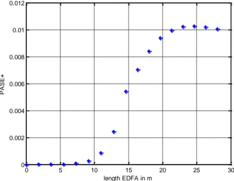
Figure 4.5 The forward travelling ASE of configuration-1---42
Figure 4.6 The backward travelling ASE of configuration-1---43
Figure 4.7 Forward-Backward pump scheme of configuration-2---43
Figure 4.8 Population density of configuration-2---44
Figure 4.9 The signal gain as a function of EDFA length with 1550 nm input signal and 7mW pump signals applied at z=0 and z=15 m in configuration-2-45 Figure 4.10 Noise Figure of configuration-2---45
Figure 4.11 The forward travelling ASE of configuration-2---46
Figure 4.12 The backward travelling ASE of configuration-2---46
Figure 4.13 Backward-Backward pump scheme of configuration-3---47
Figure 4.14 Population density of configuration-3---47
Figure 4.15 The signal gain as a function of EDFA length with 1550 nm input signal and 7mW pump signals applied at z=0 and z=15 m in configuration-3-48 Figure 4.16 Noise Figure of configuration-3---48
Figure 4.17 The forward travelling ASE of configuration-3---49
Figure 4.18 The backward travelling ASE of configuration-3---49
XIII
Figure 4.20 Population density of configuration 4---51
Figure 4.21 The signal gain as a function of EDFA length with 1550 nm input signal and 7mW pump signals applied at z=0 and z=15 m in configuration-4-51 Figure 4.22 Noise Figure of configuration-4---52
Figure 4.23 The forward travelling ASE of configuration-4---52
Figure 4.24 The backward travelling ASE of configuration-4---53
Figure 4.25 Configuration 5---55
Figure 4.26 Population density of configuration 5---56
Figure 4.27 Signal gain as a function of EDFA length at configuration-5---57
Figure 4.28 Noise Figure of configuration-5---57
Figure 4.29 The forward travelling ASE of configuration-5---58
Figure 4.30 The backward travelling ASE of configuration-5---58
Figure 4.31 Configuration-6---59
Figure 4.32 Population density of configuration 6---60
Figure 4.33 Signal gain as a function of EDFA length at configuration-6---61
Figure 4.34 Noise Figure of configuration-6---61
Figure 4.35 The forward travelling ASE of configuration-6---62
Figure 4.36 The backward travelling ASE of configuration-6---62
Figure 4.37 Configuration-7---63
Figure 4.38 Population density of configuration-6---64
Figure 4.39 Signal gain as a function of EDFA length at configuration-7---65
Figure 4.40 Noise Figure of configuration-7---65
Figure 4.41 The forward travelling ASE of configuration-7---66
XIV
LIST OF APPENDIX
A.1 Matlab code for configuration-1---83
A.1.1 Spedfa1(y) for configuration-1---83
A.1.2 Spedfa2(y) for configuration-1---84
A.1.3 Solution for configuration-1---85
A.2 Matlab code for configuration-2---89
A.2.1 Spedfa1(y) for configuration-2---89
A.2.2 Spedfa2(y) for configuration-2---90
A.2.3 Solution for configuration-2---91
A.3 Matlab code for configuration-3---96
A.3.1 Spedfa1(y) for configuration-3---96
A.3.2 Spedfa2(y) for configuration-3---97
A.3.3 Solution for configuration-3---98
A.4 Matlab code for configuration-4---103
A.4.1 Spedfa1(y) for configuration-4---103
A.4.2 Spedfa2(y) for configuration-4---104
A.4.3 Solution for configuration-4---105
A.5 Matlab code for configuration-5---110
A.5.1 Spedfa(y) for configuration-5---110
A.5.2 Dpedfa(y) for configuration-5---111
A.5.3 Solution for configuration-5---112
A.6 Matlab code for configuration-6---117
A.6.1 Spedfa(y) for configuration-6---117
A.6.2 Dpedfa(y) for configuration-6---118
A.6.3 Solution for configuration-6---119
A.7 Matlab code for configuration-7---124
A.7.1 Spedfa(y) for configuration-7---124
A.7.2 Dpedfa(y) for configuration-7---125
1 CHAPTER-1
A BRIEF HISTORY OF OPTICAL FIBERS
1.1 OPTICAL FIBER HISTORY
The basic concept of amplifying a traveling optical wave was first introduced in 1962 by Geusic and Scovil (J. E. Geusic and H. E. D. Scovil, 1962). In 1963, the utilization of optical fibers in communication systems was proposed for the first time by a Japanese scientist, Jun-ichi Nishizawa, at Tohoku University (Nishizawa Jun-ichi and Suto Ken, 2004; Sendai New, 2009). One year later, optical fiber amplifiers were invented in 1964 by E. Snitzer working for American Optical Company. He demonstrated a neodymium doped fiber amplifier at 1.06 where the fiber had a core of 10 with a 0.75 to 1.5 mm cladding. The fiber has 1 m of length, and was wrapped around a flashlamp that excited the neodymium ions (C. J. Koester and E. Snitzer, 1964; S. Sudo, 1997; Becker, Olsson and Simpson, 1999; E. Snitzer and R. Woodcock, 1965). Shortly after, the first operational fiber-optical data transmission system was developed by German physicist Manfred Börner at Telefunken Research Labs in Ulm in 1965 and the first patent application for this technology was done in 1966 (Börner Manfred, 1967). Fibers became a practical communication medium when the researchers Charles K. Kao and George A. Hockham from the British company Standard Telephones and Cables (STC) proposed for the first time that attenuation could be reduced below 20 decibels per kilometer (dB/km) (Hecht Jeff, 1999). They observed that the reason for the high attenuation level in fibers was caused by impurities that could be eliminated, rather than by fundamental physical effects such as scattering. They systematically and successfuly developed the theory for the light-loss properties in optical fibers, and discovered the right material to use for such fibers — silica glass with high purity and this discovery earned Kao the Nobel Prize in Physics in 2009 (Press Release - Nobel Prize in Physics, 2009). Just after Kao’s discovery, the attenuation limit of 20 dB/km was first achieved in 1970, by researchers Robert D. Maurer, Donald Keck, Peter C. Schultz, and Frank Zimar from American glass maker Corning Glass Works.
2
By doping silica glass with titanium, they achieved an attenuation of 17 dB/km in a fiber communication line. A few years later, they produced a fiber with only 4 dB/km attenuation where germanium dioxide is used as the core dopant (1971–1985 Continuing the Tradition, General Electric Company, 2012).
Single mode fiber amplifiers doped with rare earth ions were first demonstrated in 1983 by Broer and Simpson at Bell Telephone Laboratories. The purpose of their study was to understand the physics of fundamental relaxation mechanisms of rare earth ions in amorphous hosts (J. Hegarty, M. M. Broer, B. Golding, J. R. Simpson and J. B. MacChesney, 1983; M. M. Broer, B. Golding, W. H. Heammerle and J. R. Simpson, 1986). In 1986, AT&T Bell Labs started the research and in subsequent years many groups around the world contributed to fast development of practical Erbium Doped Fiber Amplifiers (EDFAs). In 1989, newly developed InGaAsP laser diodes were used for the first time to pump EDFA at 1480nm. Without laser diode pump sources, the utilization of EDFAs in actual systems could never have been possible (M. Digonnet, 1992; Russell Philip, 2003). Again in 1989, the first undersea test of erbium doped fiber amplifiers in a fiber optic transmission cable occurred. After 1989, EDFAs be came catalyst for the new generation high capacity undersea and terrestrial fiber optic links and networks. (N. Edagawa, K. Mochizuki and H. Wakabayashi, 1989). In conjunction with recent advances, the optical amplifiers offer solutions to the high capacity needs of nowadays voice and data transmission applications (Becker, Olsson and Simpson, 1999; Russell Philip, 2003; Kuroda, 2012).
3
CHAPTER-2 OPTICAL COMMUNICATION 2.1 INTRODUCTION
This chapter is devoted to review the fundamentals of optical communication theory and devices where optical sources, optical detectors, optical communication systems and optical passive components are explained.
2.2 OPTICAL COMMUNICATION THEORY AND DEVICES
Figure 2.1 shows a general optical communication system which consists of mainly three components; transmitter, channel and the receiver. In the transmitter part, basically, the electrical signal in form of a serial bit stream is presented to a modulator that encodes the data appropriately. A light source, la-
Figure 2.1 Optical Transmission (Harry J.R. Dutton, 1998).
ser or Light Emitting Diode – LED, driven by the modulator then sends the optical bits into the fibre transmission channel medium. In the channel, the light travels down the fibre where it may experience dispersion due to the different wavelengths in the optical wave packet. In the receiver part, the light is fed to a detector and converted back to the electrical signal in form of a serial bit stream. The signal is then amplified and fed to another detector, which isolates the individual state changes and their timing. It then decodes the sequence of state changes and reconstructs the original bit stream (Jagtar, 2011; B.P. Lathi, 1989; Harry J.R. Dutton, 1998).
4 2.2.1 OPTICAL SOURCE
2.2.1.1 Light-Emitting Diodes (LEDs)
Light-emitting diodes (LEDs) have been utilized in electronic equipment as indicator lights for decades due to their small size, durability and energy efficiency. (S. Nakamura, T. Mukai, and M. Senoh, 1994; N. Narendran, Y. Gu, J.P. Freyssinier-Nova, and Y. Zhu, 2005). In addition to this, LEDs offer a vast amount of new possibilities for product design, as compared to the traditional light sources (E.F. Schubert and J.K. Kim, 2005). One of the problems with controlling the light output from LEDs is that the technology itself has some inherent nonlinearities where both the amount of current and the temperature of the device will change the properties of the resulting illumination (Andres Thorseth, 2011). In its simplest form, an LED is a forward-biased p–n junction where radiative recombination of electron–hole pairs in the depletion region generates light. Some of the generated light escapes from the device and can be coupled into an optical fiber where this emitted light is incoherent having a relatively wide spectral width (30–60 nm) and a relatively large angular spread. (Govind P. Agrawal, 2002; J. Gower, 1993).
2.2.1.2 Light Amplification by the Stimulated Emission of Radiation (Lasers)
According to the emission theory of Einstein, energy in the form of a photon can be absorbed or emitted through carrier transitions between different energy levels where a monochromatic light wave travelling through the atoms with two energy levels having energy difference equal to the energy of the incident photon could induce the transition of atoms from a higher level to a lower energy level accompanied by emission of photons having exactly the same energy as the injected ones. Here, it is assumed that the population density in the upper level is bigger than the population density in the lower level. This is illustrated in Figure 2.2 (Xing, Cheng, 2011).
5
Figure 2.2: Stimulated emission in a two level atom. (Xing, Cheng, 2011).
Lasers can be classified according to their gain (amplifying material) medium such as gas lasers, dye lasers, solid state lasers, semiconductor lasers etc. (A. Yariv, 1989; E. Hecht, 2002). Solid state lasers use crystals as their gain medium where flashlamps having the appropriate emission wavelength are commonly placed inside the laser cavity and provide pumping light incident on the crystal. Thus, these kind of lasers are sometimes named as the optically pumped lasers. Ruby laser is the first functional solid state laser in the history and widely studied after that (Xing, 2011; T. H. Maiman, 1960).
2.2.2 OPTICAL DETECTORS
2.2.2.1 Photoconductors
Photoconductors are the simplest optical detectors consisting of a piece of (undoped) semiconductor material with electrical contacts attached where voltage is applied across these contacts. When a photon arrives in the semiconductor it is absorbed and an electron/hole pair is created. Due to the electric field between the two contacts, electron and hole each migrates separately towards the positive and the negative contact, respectively. Thus the resistance of the device varies with the amount of light falling on it. (Harry J.R. Dutton, 1998).
6
Figure 2.3: Photoconductive Detector-Principle (Harry J.R. Dutton, 1998).
2.2.2.2 Photodiodes
Photodiodes convert light directly to the electric current where an ideal (p-i-n) diode can convert one photon to one electron of current. This means that the output current obtained from such a device is very small and an external amplifier is needed before the signal is received (Harry J.R. Dutton, 1998).
Photodiodes are pn-junction diodes fabricated for the purpose of light detection having oppositely doped regions on a semiconductor substrate where these adjacent regions of opposite impurity doping result in the formation of a space charge region being free from charge carriers and having high impedance. Most pn junction photodiodes are fabricated using silicon or germanium and they exhibit high sensitivity for detecting visible and near wavelengths at room temperature (Abid Kamran, 2011; Melchior, H, 1973). When light falls on a pn-junction photodiode, the photons with higher energy than the band-gap energy of the material, generate electron-hole pairs. Photodiodes have two working modes; photoconductive or photovoltaic mode. Minimum dark current is seen in photovoltaic mode, whereas fast switching speed is seen in photodiodes when working in the photoconductive mode (Wilson, J.S, 2003).
2.2.2.3 Phototransistors
Phototransistors are photodiode-amplifier combinations integrated within a single silicon chip. These are combined to overcome the unity gain of
7
photodiodes. The typical gain of a phototransistor can range from 100 to over 1500. While the signal from a photodiode can always be amplified through use of an external op-amp or other circuitry, this approach is often not as practical or as cost-effective as the use of phototransistors. The phototransistor can be viewed as a photodiode whose output photocurrent is fed into the base of a conventional small-signal transistor. While not required for operation of the device as a photodetector, a base connection is often provided, allowing the option of using base current to bias the transistor. Phototransistors are often employed as the detector element for optoisolators and transmissive or reflective optical switches (http://www.farnell.com/datasheets/1674282.pdf).
2.2.3 OPTICAL COMMUNICATION SYSTEMS
2.2.3.1 Fibre Distributed Data Interface (FDDI)
FDDI was developed by the American National Standards Institute (ANSI) where originally it was proposed as a standard for fibre optical computer I/O channels. But later it has become a generalised standard for operation of a LAN at one hundred megabits per second. (Harry J.R. Dutton, 1998).
2.2.3.2 Synchronous Optical Network (SONET) and SDH
Synchronous Digital Hierarchy (SDH) is a multiplexing standard used all over the world except in the North America and Japan. The corresponding protocol for SDH in these areas is Synchronous Optical Networking (SONET) with relatively minor differences (Alwayn, Vivek, 2004).
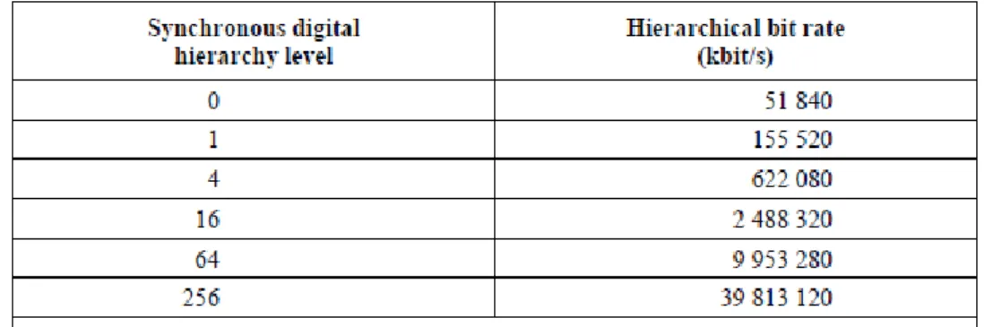
SDH defines a multiplexing hierarchy, seen in Figure 2.4, that begins with a E-carrier link (see figure 2.4 and table 2.1) and ends up with a so called STM-N (see table 2.2) frame. (European Telecommunications Standards Institute (ETSI), 2011).
8
Figure 2.4: SDH multiplexing structure as defined by the European Telecommunications Standards Institute where VC-Virtual Container, TU- Tributary Unit, TUG- Tributary Unit Group, C-Container, AU- Administrative Unit, AUG- Administrative Unit Group, STM- Synchronous Transport Module (ETSI 300 147 [21] multiplexing structure; ITU-T G.707/Y.1322 01/2007).
STM-1 is adopted as the first level of the SDH hierarchy at a rate of 155520 kb/s by the ITU. Higher SDH bit rates can be obtained as integer multiples of the first level bit rate (see table 2.2) where SDH was designed to be universal in allowing the transport of a large variety of signals. In North America, the SONET specifications were based on the 51840 kb/s Synchronous Transport Signal level 1 (STS-1) signal (A.D.Brandt, 2006).
9
Table 2.2: SDH hierarchical bit rates (ITU-T G.707/Y.1322 (01/2007))
2.2.3.3 Wavelength Division Multiplexing (WDM)
WDM is the technology where multiple wavelengths of light (multiple channels) are launched into a single optical fibre with the advantage of no additional fibre link has to be installed, but rather modifications made to the network at its nodes, allowing for a more scaleable and easy upgradeable network. DWDM (Dense Wavelength Division Multiplexing) is a denser version of WDM resulting from advances made in the tuning of lasers and wavelength filtering (S.Kempainen, 1998). Due to the intensive research and development studies, the WDM technology is advancing fastly. (Ying Lu, Okan K.Ersoy, 2003; M. S. Ab-Rahman, and S. Shaari, 2009).
In the WDM based optical access networks, wavelength selective optical add/drop filters are required for adding and dropping a particular wavelength (M. S. Ab-Rahman, and S. Shaari, 2009). In these type of WDM optical network, DWDM technology is necessary for maximizing the limited transmission bandwidth where add/drop filter used in DWDM based optical networks should have a good reflection characteristic, a temperature stability, a narrow spectral bandwidth, and a low implementation cost (Ab-bou, F.M., H.Y. Wong, C.C. Hiew, A. Abid and H.T. Chuah, 2007). Due to these reasons, although many researchers have been proposed various technologies for implementation of the add/drop filters, their cost is too expensive to apply for DWDM based optical access networks. (P. S. Andre, J. L. Pinto, T. Almedia, and M. Pousa, 2002; M. S. Ab-Rahman, and S. Shaari, 2009). However “DWDM is the only technology that enables full network flexibility
10
and adaptability at speeds of 100G and beyond, quick service turnup to meet changing bandwidth requirements, and ultra-low latency connectivity. Facilitated by the platforms, carriers can enjoy more flexible transmission, quicker service provisioning, more reliable networks, and easier maintenance, to provide better services and generate more profits” (http://www.huawei.com/; http://www.alcatel-lucent.com).
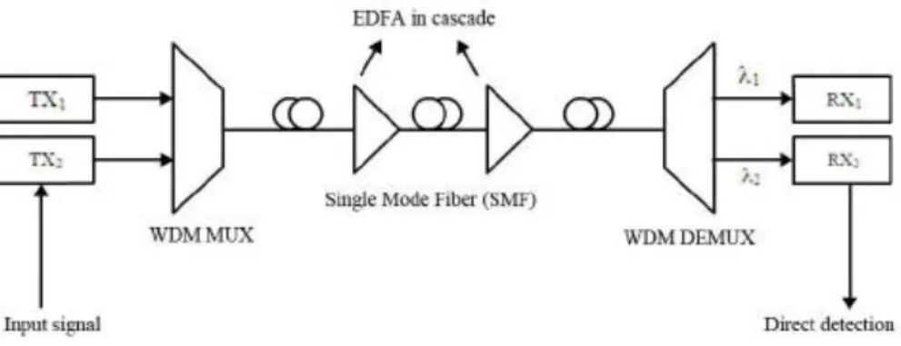
Figure 2.5: Block diagram of a WDM system (Perenyi Marcell, 2009)
WDM is basically an analogy of Frequency Division Multiplexing in the infrared domain where independent streams of data are modulated using different frequencies and sent through the same piece of fiber (see figure 2.6) (Perenyi Marcell, 2009; Achyut K. Dutta, Niloy K. Dutta, Masahiko Fujiwara, 2004; Krishna M. Sivalingam, Suresh Subramaniam, 2002). Multiplexing and demultiplexing optical signals is an essantial component in WDM networks where optical signals must be split and joined regarding the frequency of the signal. There are two main types of demultiplexers, active and passive. Arrayed waveguide gratings, an example of a passive demultiplexer, can typically be also used as multiplexers (J.P. Laude and C-N. Zah, 1984; Arjen R. Vellekoop and Meint K. Smit, 1991). Acoustically tunable filters, an example of an active demultiplexer, have the ability to dynamically select multiple wavelengths (Perenyi Marcell, 2009; David A. Smith, Jane E. Baran, John J. Johnson and Kwok Wai Cheung, 1990).
At the receiver, several filters can be used to seperate (demultiplex) the signals from each other (Perenyi Marcell, 2009; Achyut K. Dutta, Niloy K. Dutta,
11
Masahiko Fujiwara, 2004; Krishna M. Sivalingam, Suresh Subramaniam, 2002) in which demultiplexing can be done by diffraction based demultiplexers or interference based demultiplexers. In addition to these the most often used demultiplexing approach is the Arrayed Waveguide Grating (Govind P. Agrawal, 2002).
“Literature distinguishes dense and coarse WDM technologies depending on the spacing of the wavelength channels: the Dense WDM recommendation described in ITU-T G694.1 supports channel spacing values of 100, 50, 25 and 12.5 GHz with, respectively, allowing approximately 115, 229, 458 and 916 channels in the C and L bands. (table 2.3) The Coarse WDM scheme (ITU-T G694.2) defines 18 channels with channels spacing larger than 2 THz in the spectral bands by the letters O, E, S, C and L” (Spectral grids for WDM applications: DWDM freguency grid, ITU-T Recommendation G.694.1 June 2002; Spectral grids for WDM applications: CWDM freguency grid, ITU-T Recommendation G.694.2 December 2003)
Table 2.3: Transmission windows used in optical fibers (ITU-T Recommendation G.694.2)
Band Description Wavelength Range
O band original 1260 to 1360 nm
E band extended 1360 to 1460 nm
S band short wavelength 1460 to 1530 nm
C band conventional ("erbium window") 1530 to 1565 nm
L band long wavelength 1565 to 1625 nm
U band ultra long wavelengths 1625 to 1675 nm
DWDM refers originally to optical signals multiplexed within the 1550-nm band where erbium doped fiber amplifiers (EDFAs) are effective for wavelengths between approximately 1525-1565 nm (C band) or 1570-1610 nm (L band). EDFAs were originally developed to replace SONET/SDH optical-electrical-optical (OEO) regenerators since EDFAs, regardless of the modulated bit rate, can amplify any optical signal in their operating range. In terms of multi- wavelength signals (assuming that EDFA has enough pump signal energy available), it can amplify as many optical signals as can be
12
multiplexed into its amplification band. EDFAs therefore allow a single-channel optical link to be upgraded in bit rate by replacing only equipment at the ends of the link, while retaining the existing EDFA or series of EDFAs through a long haul route. Furthermore, single- wavelength links using EDFAs can similarly be upgraded to WDM links at reasonable cost where the EDFAs cost is thus leveraged across as many channels as can be multiplexed into the 1550-nm band (S. M. Nazmul Mahmud, Abdul Aoual Talukder, 2009)
2.2.3.4 Free Space Optics (FSO)
FSO systems use infra-red laser sources for the transmission of data between the transmitter and the receiver where they can transmit up to 1.25 Gbps over a maximum distance of 4 km. Since these systems use optical signals, it is not required to get radio spectrum licensing. FSO systems also have low installation costs. However, in poor weather conditions, they may shut down. Morever, FSO systems are only useful in short distance private applications due to their point-to-point nature (Oladeji Akanbi, 2006; Carl Brannlund, 2008).
2.2.4 OPTICAL PASSIVE COMPONENTS
2.2.4.1 Fiber
Figure 2.6: Schematic of a step index optical fibre. (Erji Mao, 2000).
An optical fiber is a cylindrical waveguide made of low-loss materials, such as silica glass, carries light along its length. The core in which the light
13
propagates and being guided is embedded in a cladding of slightly lower refractive index (see figure 2.6). Light rays coming at angles greater than the critical angle at the core-cladding interface undergo total internal reflection. Thus, these rays are guided and propagate inside the core (Erji Mao, 2000; Y. Weissman, 1992; Ankush Kumar, 2009). The cladding is usually coated with a tough resin buffer layer. In some cases this layer may be further surrounded by a jacket layer made of glass. These layers add only mechanical strength to the fiber and do not change to its optical wave guide properties. In order to reduce cross-talk between the fibers sometimes light-absorbing glass is utilized between the fibers in rigid fiber assemblies. (Light collection and propagation, National Instruments' Developer Zone, National Instruments Corporation, 2007; E. Hecht, 2002).
2.2.4.2 Couplers
Couplers are simple passive optical components used for spliting or combining signals where it consists of n input and m output ports. A 1 x m coupler is called a splitter and an n x 1 coupler is called a combiner. Figure 2.7, 2 x 2 coupler is described where a part of the first input signal is directed to the first output port and the rest to the second output port. In a similar way a part of the input second input signal is guided to both output ports. The fractions directed to output ports can be either equal or non-equal (Henrique, et al, 2002).
14 2.2.4.3 Isolators and Circulators
Isolators (see figure 2.8a) are devices that allow transmission only in one direction and block the transmissions in the reverse direction. In order to prevent reflections from amplifiers or lasers. Typically the insertion loss, i.e. the loss in the forward direction is around 1 dB and the isolation, i.e. the loss in the reverse direction, is approximately 40 to 50 dB.
A circulator is a device similar to an isolator having multiple ports. Figure 2.8b) shows a circulator with input and output ports. A signal from each port is directed to the next adjoining port and blocked in all the other ports (see Figure 2.8c). Circulators can be used as a component in optical add/drop multiplexers and optical cross-connects (ttp://www.lightreading.com).
Figure 2.8: a) Isolator, b) Circulator, c) Logical scheme of a three port circulator (ttp://www.lightreading.com).
2.2.4.4 Filters
In order to filter or multiplex wavelength dependent we need to separate different frequencies from the signal. The principle idea for doing this depends on that some wavelengths are delayed in phase compared to other wavelengths. This is done by directing them through a longer path (Henrique, et al, 2002).
The key parameters of filters are insertion loss and passband flatness where insertion losses should be low and independent of polarization and temperature and passband should be flat and passband skirts should be as sharp as possible. As seen in figure 2.9t he flatter the passband and sharper the passband skirts,
15
we obtain smaller crosstalk energy passing through the adjacent channels (R. Ramaswami, K. N. Sivarajan, 1998).
16 CHAPTER-3
ERBIUM DOPED FIBER AMPLIFIERS 3.1 INTRODUCTION
The development of erbium doped fiber amplifiers (EDFAs), started in the mid 1980s, have been a major impetus on the growth of fiber communications with wavelength division multiplexing (WDM) and an important catalyst to the research on active-fiber technology in the third optical telecommunications window near 1.55 µm wavelength region where the loss of silica fibers is minimum (Mears, Reekie, Jauncey, and Payne, 1987; Morkel and Laming, 1989; M. Nakawaza, Y. Kimura and K. Suzuki, 1989; Giles and Desurvire, 1991; Fouli, 2002). EDFAs are now common components of lightwave transmission systems and have been widely used in optical communications (Giles and Desurvire, 1991; Fouli, 2002; Kuroda, 2012) due to the advantages they provide. It is possible to directly amplify optical data without conversion to electrical data by using EDFAs (Kuroda, 2012). Polarization independent high gain and low noise in the optical communication networks and providing a broadband amplification of radiation whose wavelength is in the so-called third window make EDFAs an important tool for building compact and practical devices for diverse applications in fiber-optic communication (Morkel and Laming, 1989; N. A. Olsson, 1989; Kemtchou, Duhamel and Lecoy, 1997).
“The erbium doped fiber systems results into important advantages for information processing and transmission like: possibility of easy integration, highly efficiency and gain, immunity to crosstalk, low noise and high saturation output power”(Agrawal, 1995 & 1997; Desurvire, 1995; Sterian, 2006).
17 3.2 EDFA BASICS
3.2.1 Three-Level System for EDFAs
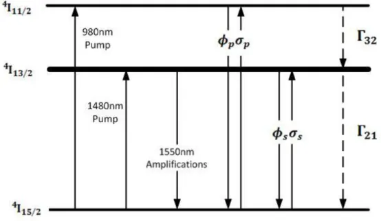
The general modeling of the erbium-doped fiber amplifier can be considered as a pure three level atomic system (Becker, Olsson and Simpson, 1999: 131; Simpson and Becker, 1987:12).
Figure 3.1: Simplified three level energy diagram of Er3+ for the amplifier model. The transition rates between levels 1-3 and 1-2 are proportional to the populations in those levels and to the product of the pump flux - pump cross-section and signal flux - signal cross-section , respectively. The spontaneous transition rates of the ion (including radiative and nonradiative contributions) are given by and (Muhyaldin, 2009; Becker, Olsson
and Simpson, 1999: 132; Desurvire, 1994; Bjarklev, 1993).
For EDFAs, the stimulated emission is the main amplification mechanism where the population inversion is achieved by optical pumping. During this process, electrons that exist at higher energy levels are raised to the excited states by pump photons (Muhyaldin, 2009; Becker, Olsson and Simpson, 1999: 131; Desurvire, 1994; Bjarklev, 1993; Ghatak and Thyagarajan, 1998; Giles and Desurvire, 1991).
18
The configuration depicted in Figure 3.1 is known as the three level system model where the ground state is denoted by 1, an intermediate state labeled by 3 (into which energy is pumped), and another intermediate state by 2. State 2 often has relatively a longer lifetime for good amplifiers where it is referred as metastable level. For the considered model, state 2 is the upper level of the amplifying transition and state 1 is the lower level. The populations of the levels are labeled , and . The amplification is obtained incase of a population inversion between states 1 and 2 where at least half of the total population of erbium ions at level 1 needs to be excited to level 2 to have population inversion (Becker, Olsson and Simpson, 1999: 131;Giles and Desurvire, 1991).
“The incident light intensity flux at the frequency corresponding to the 1 to 3 transition (in number of photons per unit time per unit area) is denoted by and corresponds to the pump. The incident flux at the frequency corresponding to the 1 to 2 transition (in photons per unit time per unit area) is denoted by and corresponds to the signal field. The change in population for each level arises from absorption of photons from the incident light field, from spontaneous and stimulated emission, and from other pathways fort he energy to escape a particular level. In particular, we write as the transition probability from level 3 to level 2. This is the sum of the nonradiative and radiative transition probabilities, and in practice, for the most typical cases, is mostly nonradiative. is the transition probability from level 2 to level 1. In the case of the
(level 2) to (level 1) transition, is mostly
due to radiative transitions. This is due to the fact that there are, for , no
intermediate states between levels 1 and 2 to which ions excited to level 2 can relax. It was defined ⁄ , where is the lifetime of level 2.”(Becker, Olsson and Simpson, 1999: 133)
The absorption cross section for the transition between state 1 to state 3 is denoted by , and the emission cross section for the transition between state 2 to state 1 is denoted by in Figure 3.1. Absorption and emission cross
19
sections are considered equal for transitions between individual nondegenerate states (Bao and Hong Son, 2004; Becker, Olsson and Simpson, 1999: 133).
“The rate equations for the population changes are written as”(Becker, Olsson and Simpson, 1999: 133; Desurvire, 1994)
“In steady-state situation, the time derivatives will all be zero,
and the total population N is given by”
(Becker, Olsson and Simpson, 1999: 132,133)
20
When is large (corresponding to a speedy transition from level 3 to level 2) compared to the effective pump rate into level 3, then the value of and is very close to zero. Thus, the population of erbium ions is mostly in levels 1 and 2. From Equation 3.6, the population of level 2 can be written as:
(
)
Then, from Equation 3.5, the populations , and population inversion ( ) can be derived as:” (Muhyaldin, 2009; Becker, Olsson and Simpson, 1999: 134)
3.2.2 The Overlap Factor and
“In order to obtain the effective area of the absorption and emission cross sections, the transverse shape of the optical mode and its overlap with the transverse erbium ion distribution profile are very important since only the portion of the optical mode that overlaps with the erbium ion distribution will impact on absorption and emission. The overlap factor is defined as a parameter to describe the relation between the optical mode and the erbium ion distribution.” (Xia, 2002; S. Park, Ahn, Ko, W. Lee, Oh, M. Lee and H. Park, 2013).“Generally, part of the optical mode will propagate in the cladding but erbium ions are typically doped in the core of the fiber. Therefore, the overlap factor is always less than 1” (Xia, 2002).
21
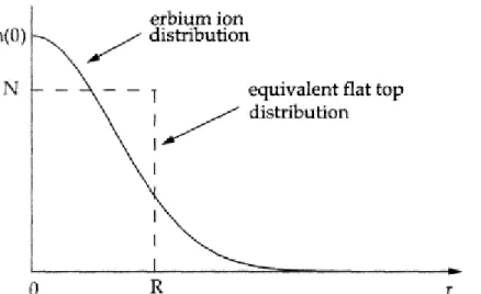
The effective cross-sectional area is decided by the shape of the erbium ion distribution and can be obtained by , where R is the equivalent flat top radius of the erbium ion distribution. Since the actual transverse distribution of erbium ions is hard to obtain, is usually used to simply the calculation in the mode. Figure 3.2 shows an example of an equivalent flat top distribution and the actual erbium ion distribution. The radius R of the flat top distribution is deterrnined by the geometric profile of the actual erbium ion distribution”(Xia, 2002).
Figure 3.2: “Example of a radial distribution of the erbium ion density in a single-mode fiber and the equivalent “flat top” distribution, which has a constant ion density N stretching from r=0 to r=R.”(Xia, 2002; Becker, Olsson and Simpson, 1999: 142)
3.2.3 Lifetimes
“The lifetime of a level is inversely proportional to the probability per unit time that the ion will exit from that excited level. When there are several pathways for the population to decay, the total probability is the sum of the individual probabilities for each pathway. The two main pathways for decay are radiative and non-radiative, and hence the lifetime is given by,
22
where is the total lifetime, is the radiative lifetime, and is the
non-radiative lifetime. (Desurvire, 1994)” “The non-radiative lifetime arises from the fluorescence from an excited level to all the levels below it. Non-radiative lifetime depends largely on the glass composition and the coupling between the vibrations of the lattice ions and the states of the rare earth ions. (Lidgard at all, 1991)”
3.2.4 Linewidths and Broadening
“Linewidth represents a finite spectrum of the gain in the wavelength domain. This happens due to broadening of the energy states, i.e., each of the states actually is a collection of many closely spaced energy levels. The homogeneous, or natural, broadening arises from the lifetime and depends on both radiative and nonradiative processes (Milonni, Eberly, 1988).” “Hence, the faster the lifetime the broader the state. The inhomogenous broadening is a measure of various different sites in which an ensemble of ions can be situated. An inhomogenous line is thus a superposition of a set of homogeneous lines. Such homogeneous and inhomogenous lineshapes are shown in figure 3.3 respectively. In the presence of a strong signal that saturates the transition, the absorption or emission lineshapes will be affacted in a different way, depending on whether the line is homogeneously or inhomogeneously broadened. In glasses, both the homogeneous and inhomogeneous broadening can be quite large, as compared to crystals (Becker, Olsson and Simpson, 1999).” “In silica fibres where the photon energy is rather strong and electron-photon coupling strength is significant, the homogeneous broadening is quite large. The inhomogeneous broadening is also large due to multiplicity of sites and environments available to the ion (Todorikki, Hirao and Soga, 1992).”
23
Figure 3.3: (a) A homogenously broadened line for a collection of ions with identical transition wavelengths and lifetimes. (b) An inhomogeneously broadened line made up of a collection of homogeneously broadened lines with different centre wavelengths and linewidths. (Becker, Olsson and Simpson, 1999)
3.2.5 Two-Level System for EDFAs
“Having reduced the three-level system to an effective two-level system, we can write the rate equations so as to involve only the total population densities of multiplets 1 and 2. ( ) ( ) ( ) ( )
Where , , and represent the signal and pump absorption and emission cross section, respectively.”(Becker, Olsson and Simpson, 1999: 146; Pedersen, Bjarklev, Povlsen, Dybdal and Larsen, 1991; Song, Park, Lee and Kim, 2012).“Since the total population density N is given by
24 We have
and only one of the equations from system 3.9 is an independent equation. We can calculate , for example, in terms of the signal and pump intensities. is then simply given by . It was found from equations 3.9, for the case of one pump field an done signal field, that the population density , as a function of position z along the fiber, is given by
( ) ( )
In general, we will assume that N is independent of z. The pump and signal propagation equations are then written, in a very similar fashion, as
( ) ( )
Stimulated emission from level 2 contributes to field growth, absorption from level 1 contributes to field attenuation. The equations needed to simulate the amplifying properties of the fiber are thus the population equation and the propagation equations, one for each field. The condition for population inversion, , in the presence of a small signal field, corresponds to the pump being greater than the threshold value:
25
The pump threshold that corresponds to signal gain at the signal wavelength ( is slightly different is equal to
(
)
The equations above can be easily generalized to the case of multiple signals and multiple pumps.”(Giles and Desurvire, 1991; Giles, Burrus, DiGiovanni, Dutta and Raybon, 1991; Becker, Olsson and Simpson, 1999: 147) “For the case of several signals and several pump , the population equation becomes ∑ ∑ ∑ ∑
The field propagation equations are identical to those of equations 3.13, with appropriate cross sections. Such multisignal system of eguations will be used when computing, for example, the spectral distribution of the ASE or the amplification of multiple-signal channels in a WDM system.”(Becker, Olsson and Simpson, 1999: 147)
26 3.2.6 Amplified Spontaneous Emission
“Spontaneous emission is an important phenomenon in optical amplifiers. The excited erbium ion can spontaneously relax to the ground state and emit a photon that is unrelated to the input signal wavelength. In an EDFA, photons at random wavelengths are generated and propagate in both forward and
backward directions. These photons can be further amplified along the rest of the EDF as signals and therefore, they are referred to as ASE (amplified spontaneous emission).” (Xia, 2002)“Spontaneous emission will result in randomly phased, incoherent radiation travelling in al1 direction. Therefore. those spontaneously generated photons which undergo gain in the fïber
amplifier and travel in the same direction as the signal light. form a background noise that adds to the signal light. This background noise is referred ro as amplified spontaneous emission. This is an inevitable phenornenon which degrade the signal-to-noise ratio (SNR) of the received signal.”(Heng Foo, 1999)
The basic element of ASE power is the equivalent noise power, which is defined as the power generated in a point of EDF by spontaneous emission at frequency v and in a bandwidth of . Since there are two independent polarizations for a given frequency, the equivalent noise power can be expressed as:”
(Xia, 2002)
27
3.3 MODELING AND COMPLEX EFFECTS
3.3.1 Gain for EDFA
“Gain is the main chracteristic of an amplifier. The EDFA gain is defined as the ratio of the output signal power to the input signal power as shown in Equation (3.18). It is calculated by integrating the gain coefficient g( ) over the length L of the erbium-doped fibre. The gain coefficient g() is calculated by summation of both the emission coefficient, , multiplied by the fractional populations of the ions in the excited state, N2, and the absorption
coefficient, , multiplied by the fractional populations of the ions of the first excited and ground states of erbium, N1, the terms
and are shown in Equation (3.19)” (Muhyaldin, 2009; Zyskind and Nagel)
∫
∫ ( )
“The spectra of the emission and absorption coefficients of an erbium doped Ge/Al/P silica fibre are shown in Figure 3.4. The gain coefficient can be expressed in units of dB/m. The terms mentioned are used in the numerical simulations, which focused on the analysis of the dynamic behaviour of cascaded EDFAs in WDM optical networks. These values are provided by Highwave-Technologies of France.” (Muhyaldin, 2009; www.highwave-tech.com, 2002)
28
Figure 3.4: EDFA gain performance as a function of the input signal powers in dBm, at wavelength 1549.2 nm, at saturation for pump powers of 40, 65, 100 mW(Muhyaldin, 2009; www.highwave-tech.com, 2002)
“Figure 3.5 shows the curves of the gain G versus the pump power Pp, where we take the signal Ps= 1 W, ion concentration
=1.0x ,
ionconcentration , 2.0x , and waveguide length z=1,2,3 cm.” (Wang, Sheng Ma, Li, Zhang, 2008)
Figure 3.5: Curves of gain G versus pump power (Wang, Sheng Ma, Li, Zhang, 2008).
29 3.3.2 Gain as Function of Fiber Length
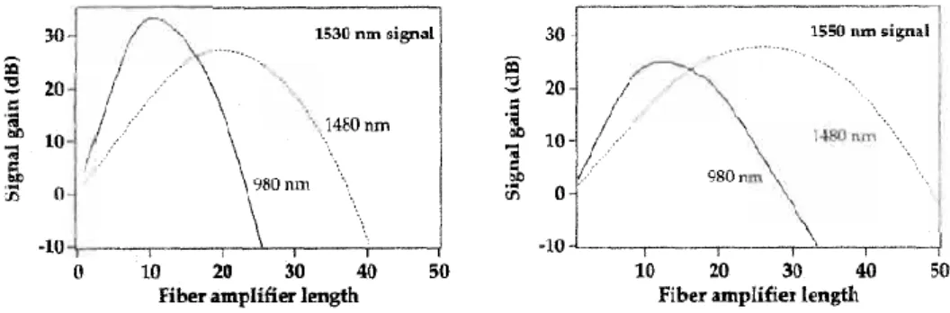
“Figure 3.6 shows the signal gain at 1550 nm, for both 980 nm and 1480 nm pumping and 40 mW of pump power, as a function of the erbium-doped fiber length, for erbium-doped Al-Ge silica fiber. Interestingly, for the 1550 nm signal, the 1480 nm pump provides a higher gain than the 980 nm pump at equal pump powers. This was noted in previous simulations.” (Povlsen, Bjarklev, Lumholt, Vendeltrop-Pommer, Rottwitt and Rasmussen, 1991)
Figure 3.6: Signal gain at 1530 nm (left) and 1550 nm (right) for 1480 and 980 nm pumping of erbium-doped Al-Ge silica fiber, as a function of fiber amplifier length. The launched pump power is 40 mW and the launched signal power is -40 dBm (Povlsen et al, 1991).
“The 1480 nm pump can maintain the necessary inversion levels ( 0.40 for this particular fiber) over significantly longer lengths than the 980 nm pump. The reason for this is the higher quantum efficiency of 1480 nm pumping. This allows the signal to grow to a higher maximum value. The situation is reversed in the case of the 1530 nm signal. Since 1530 nm signal requires high inversions ( 0.53) and benefits from very high inversion levels, the 980 nm pump with its higher inversion capabilities can reach higher small signal gains than a 1480 nm pump, not with standing the greater quantum efficiency of latter. (Becker, Olsson and Simpson, 1999: 169) For higher input powers (e.g., -10 dBm), the fiber will be in a saturation regime where the inversion is reduced. In that case the higher quantum efficiency of the 1480 nm pump is the dominant factor and will give a higher gain at 1530 nm than the 980 nm pump. At high pump powers (for this particular fiber geometry) such as 40mW, the
30
maximum gain is achieved within a relatively broad range of fiber lengths. At low powers, the optimal length is in a much narrower range, as is shown in Figure 3.7.”(Becker, Olsson and Simpson, 1999: 169, Papannareddy, 2002:87)
Figure 3.7: Signal gain at 1530 nm (left) and 1550 nm (right) for 1480 nm and 980 nm pumping of erbium-doped Al-Ge silica fiber, as a function of fiber amplifier length. The launched pump power is 10 mW and the launched signal power is -40 dBm. From numerical simulations(Becker, Olsson and Simpson, 1999: 169; Papannareddy, 2002:88).
3.3.3 Noise in EDFA
“Most, if not all, applications of photons and lightwave signals in communications, sensors, signal processing, etc., require the detection and subsequent conversion of the an electrical signal. In this process, the useful signal will be corrupted by noise and the ultimate sensitivity and performance of the system is limited by the noise characteristics.” (Becker, Olsson and Simpson, 1999: 201)“If EDFAs can compensate for the loss suffered while propagating through a fiber, the question that arises in one’s mind is whether it is possible to traverse an arbitrarily long distance in the fiber by periodic amplification along the fiber link provided that the dispersion effects do not limit the distance. This is, in fact, not possible, due to the addition of noise by each amplifier, as discussed below.
In an EDFA, population inversion between two energy levels of erbium ion leads to optical amplification by the process of stimulated emission. As
31
mentioned earlier, erbium ions occupying the upper energy level can also make spontaneous transitions to the ground state and emit radiation. This radiation appears over the entire fluorescent band of emission of erbium ions and travels in both the forward and backward directions along the fiber. Just like the signal, the spontaneous emission generated at any point along the fiber can be amplified as it propagates through the population-inverted fiber. The resulting radiation is called amplified spontaneous emission (ASE). This ASE, which has no relationship with the signal propagating through the amplifier, is the basic mechanism leading to noise in the optical amplifier. (Thyagarajan and Ghatak, 2007)
Figure 3.8: An EDFA amplifies an input signal, and along with the amplified signal there is a background ASE that constitutes the noise of the amplifier. Any ASE not coincident with the signal wavelength can be filtered using an optical filter. However, ASE within the signal band cannot be filtered and constitutes the minimum noise added by the amplifier.
Figure 3.8 shows the spectrum at the input of an EDFA and the output from the EDFA. At the output we have both the amplified signal and a background ASE. The ASE appearing in a wavelength region not coincident with the signal can be filtered using an optical filter as shown in the figure. On the other hand, the ASE that appears in the signal wavelength region cannot be separated and constitutes the minimum added noise from the amplifier.” (Thyagarajan and Ghatak, 2007)
“If represents the signal input power (at frequency ) into the amplifier and G represents the gain of the amplifier in linear units (the corresponding gain in decibels is given by ̃=10logG), the output signal power is given by .
32
Along with this amplified signal, there is ASE power, which can be shown to be given by
where is the optical bandwidth in the frequency domain over which the ASE power is being measured (which must be at least equal to the optical bandwidth of the signal), and the spontaneous emission factor is given by”
(Becker, P.C. 2002; Thyagarajan and Ghatak, 2007; Becker, Olsson and Simpson, 1999: 204)
“Here and represent the population densities (number of atoms per unit volume) in the upper and lower amplifier energy levels of erbium in the fiber. Minimum value for corresponds to a completely inverted amplifier for which (i.e., all atoms excited to the upper level) and thus ; for partial inversion, .
“We can define the optical signal-to-noise ratio (OSNR) as the ratio of the output optical signal power to the ASE power:
(Thyagarajan and Ghatak, 2007; Becker, Olsson and Simpson, 1999: 231; R. Tenc )
where is the average power input into the amplifier (which is about half of the peak power in the bit stream, assuming equal probability of 1’s and 0’s).
33
“Amplifier noise is the ultimate limiting factor for system applications. For a lumped EDFA, the impact of ASE is quantified through the noise figure NF given by . The spontaneous emission factor nsp depends on the relative populations and of the ground and excited states as 4.21. Since EDFAs operate on the basis of a three-level pumping scheme, and
. Thus, the noise figure of EDFAs is expected to be larger than the
ideal value of 3 dB” (Agrawal, 2002; S. B. Alexander, 1987; M. W. Maeda and D. A. Smith, 1991).
“The spontaneous-emission factor can be calculated for an EDFA by using the rate-equation model discussed earlier. However, one should take into account the fact that both and vary along the fiber length because of their dependence on the pump and signal powers; hence should be averaged along the amplifier length. As a result, the noise figure depends both on the amplifier length L and the pump power , just as the amplifier gain does. Figure 3.9(a) shows the variation of NF with the amplifier length for several values of ⁄ when a 1.53 signal is amplified with an input power of
1mW. The amplifier gain under the same conditions is also shown in Figure 3.9(b). The results show that a noise figure close to 3 dB can be obtained for a high-gain amplifier pumped such that ⁄ ” (Agrawal, 2002; S. B. Alexander, 1987)
Figure 3.9: (a) noise figure and (b) amplifier gain as a function of the length for several pumping levels. (M. W. Maeda and D. A. Smith, 1991)
34
“The experimental results confirm that NF close to 3 dB is possible in EDFAs. A noise figure of 3.2 dB was measured in a 30 m long EDFA pumped at 0.98 with 11 mW of power” (T. Okoshi, 1985; Agrawal, 2002). “A similar value was found for another EDFA pumped with only 5.8 mW of pump power at 0.98 ” (Agrawal, 2002; T. G. Hodgkinson, R. A. Harmon, and D. W. Smith, 1987). “In general, it is difficult to achieve high gain, low noise, and high pumping efficiency simultaneously. The main limitation is imposed by the ASE traveling backward toward the pump and depleting the pump power. Incorporation of an internal isolator alleviates this problem to a large extent. In one implementation, 51 dB gain was realized with a 3.1 dB noise figure at a pump power of only 48 mW” (P. Poggiolini and S. Benedetto, 1994).
“The measured values of NF are generally larger for EDFAs pumped at 1.48 . A noise figure of 4.1 dB was obtained for a 60-m-long EDFA when pumped at 1.48 ” (T. Okoshi, 1985). “The reason for a larger noise figure for 1.48 pumped EDFAs can be understood from Figure 3.9(a), which shows that the pump level and the excited level lie within the same band for 1.48 pumping. It is difficult to achieve complete population inversion under such conditions. It is nonetheless possible to realize for pumping wavelengths near 1.46 . (Agrawal, 2002)
“Relatively low noise levels of EDFAs make them an ideal choice for WDM light wave systems. In spite of low noise, the performance of long-haul fiber-optic communication systems employing multiple EDFAs is often limited by the amplifier noise. The noise problem is particularly severe when the system operates in the anomalous-dispersion region of the fiber because a nonlinear phenomenon known as the modulation instability enhances the amplifier noise and degrades the signal spectrum” (S. Benedetto and P. Poggiolini, 1994; G. P. Agrawal, 1996; S. Ogita et al, 1990).