A switching model approach to stock price modeling

A SWITCHING MODEL APPROACH

TO STOCK PRICE MODELING

HANDE ORUÇ

107622004

·

ISTANBUL B·

ILG·

I ÜN·

IVERS·

ITES·

I

SOSYAL B·

IL·

IMLER ENST·

ITÜSÜ

EKONOM·

I YÜKSEK L·

ISANS PROGRAMI

TEZ DANI¸

SMANI: YRD. DOÇ. DR. ORHAN ERDEM

A SWITCHING MODEL APPROACH

STOCK PRICE MODELING

HANDE ORUÇ

107622004

Tez Dan¬¸sman¬n¬n Ad¬Soyad¬(·IMZASI):Yrd.Doç.Orhan Erdem Jüri Üyelerinin Ad¬Soyad¬(·IMZASI) :

Jüri Üyelerinin Ad¬Soyad¬(·IMZASI) :

Tezin Onayland¬¼g¬Tarih :

Toplam Sayfa Say¬s¬:

Anahtar Kelimeler (·Ingilizce) Anahtar Kelimeler (Türkçe) 1.Regime Switching Model 1.Rejim De¼gi¸stirme Modelleri 2.Geometric Brownian Motion 2.Geometrik Brown Devinimi

Abstract

In this study, we consider a nonlinear probabilistic discretized version of Geo-metric Brownian Motion (GBM) to model the stock prices traded in Istanbul Stock Exchange. By nonlinearity we mean the existence of di¤erent states in the model, namely positive return process, negative return process. As the names im-ply, each process is formed using positive and negative returns respectively. The model decides which process to use according to a probabilistic framework en-dogenously determined in the model. By means of these probabilities, this model is designed to give better …t than GBM, where the better …t is acquired by Mean Squared Errors (MSE). We obtain the results via the Monte Carlo technique using Matlab and hundred stock prices. As a result, the obtained probabilities after simulation demonstrate that positive returns tend to be followed by negative return process and vice versa.

Özet

Bu çal¬¸smada, Istanbul Menkul K¬ymetler Borsas¬’nda i¸slem gören hisse senet-lerini do¼grusal olmayan olas¬l¬kl¬ ayr¬kla¸st¬r¬lm¬¸s Geometrik Brownian Devin-imini kullanarak modellendi. Hisse senetlerini pozitif getiri ve negatif getiri olarak ikiye ay¬rarak do¼grusal olmayan model olu¸sturuldu. Model içerisinde be-lirlenen olas¬l¬klarla positif veya negatif getiri süreçleri kullan¬larak model olu¸ stu-ruldu. Olas¬l¬klar hata karelerinin ortalamlar¬minimum olacak ¸sekilde belirlendi. Sonuçlar, MATLAB yard¬m¬yla IMKB’de i¸slem gören yüz hisse senedi için Monte Carlo simulasyonu yap¬larak bulundu. Yap¬lan çal¬¸sman¬n sonucunda; pozitif ge-tirilerin negatif getirileri, negatif gege-tirilerin ise pozitif getirileri takip etti¼gi ortaya ç¬kt¬.

Acknowledgements

First of all, I would like to thank my supervisor Asst. Prof. Dr. Orhan Erdem for all his help and support. I greatly appreciate his indispensable help and I am very much indepted to him. I am very thankful to Muza¤er Akat for his valuable contributions. It is hard to express how greatful I am for the time he spent with me to improve this work. I would like to thank my family for everything and one of my best friends Fatma Aslan, I am very happy to meet her and she is always an indispensable friend for me. I want to thank Demet Demir and Murat Öztürk for their support and I would like to thank Uygar Ekin and Mehmet Evren Eynehan for data support. Finally, I would like to thank TUBITAK for scholarship.

Contents

1. Introduction 2. The Data 3. Models

3. 1.Threshold Autoregressive Model (TAR) and

Continuous Time Threshold Autoregregressive Model (CTAR) 3. 2. Markov Switching Model and

Continuous Time Markov Switching Model 3. 3. Geometric Brownian Motion (GBM)

4. The modi…ed Geometric Brownian Motion and Methodology 5. Results

6. Conclusion and Future Work 7. References

Section 1

Introduction

With the progress of …nancial markets, modeling stock prices became very popular. Stock price data are modeled in two di¤erent types: discrete and con-tinuous time processes. The analysis related to the processes which are examined as discrete time are called time series analysis and in the time domain the sim-plest time series models such as random walk, autoregressive, moving average models etc. are based on regression analysis. Since many relationships in …nance are nonlinear, these linear models are unable to capture the features of the data in …nance.

Therefore, two di¤erent types of nonlinear models are formed. On the one hand, stochastic variable models such as ARCH, GARCH models are used for modeling and forecasting volatility; on the other hand, deterministic variables models such as regime switching models allow the behaviour of a series to follow di¤erent processes at di¤erent points in time.

In recent years, regime switching models which use thresholds have become popular in …nance. As an example, we can separate the state of market into two di¤erent regimes such as "bullish" and "bearish". The special feature of these models is that the key parameters such as mean, volatility etc. tend to change according to the state of the market. Furthermore, in a regime switch-ing model, the state of the related market is divided into a …nite number of regimes. Hence, the assumption of linearity in time series analysis has been abandoned and the study of nonlinear model becomes increasingly popular. Tong (1978) has developed threshold autoregressive model (TAR) which is one class of nonlinear model. The property of this model is that the process is divided into regimes and for each regime there are di¤erent AR models. In addition to

TAR model, Markov switching model which is developed by Hamilton (1989) posits that regime switches are exogenous according to probabilities. The regime switching models are not designed to explain the reason of the regime changes oc-curance and the timing of such changes. In addition to ARCH model and Markov switching model, Hamilton and Susmel (1994) proposed the SWARCH model, a mixture of Markov-switching model and ARCH model. SWARCH model assumes di¤erent parameter values in the conditional variance equation.

All models that we mentioned above are used to estimate discrete-time sto-chastic process, in which the price changes at discrete time points. In …nancial markets, however, assets are traded at very frequent intervals of time. A rea-sonable approximation is to let the interval of time go arbitrarily close to zero, which leads to a world of continuous-time models. In addition to that, the e¢ cient market hypothesis suggests that share price should follow random walks. The continuous-time analogues of a random walk and a random walk with drift are Brownian Motion(BM) and Geometric Brownian Motion (GBM), respectively.

After BM having been invented, it has been used by the vast branch of science such as …nance, engineering etc. BM which is common to have a continuous time price process modeled in …nance was discovered by the English botanist Robert Brown in 1827. In the process of time, di¤erent types of BM are composed. For example, Phadke and Wu (1974) developed continuous time autoregressive models (CAR).

The models which are used to model discrete time series can be adapted to continuous time …nance. As ARCH and GARCH are used to model volatil-ity in discrete time series, a family of continuous-time generalized autoregres-sive conditionally heteroscedastic process, generalizing the COGARCH process of Klüppelberg et al. (2004), is introduced and studied. Additionally, Brockwell et al. (2006) developed this continuous time GARCH process and the volatility process is found to have autocorrelation function of a continuous-time

autore-gressive moving average.

As TAR model was invented in discrete time by using deterministic variable autoregressive model, it has been adapted to nonlinear GBM, as well. For this purpose, Tong and Yeung (1991), Brockwell et al. (1991) developed continuous time threshold autoregressive model (CTAR). On the other part, Gerber and Shiu (2003) and Jose(2008) tried to constitute GBM which is developed by a barrier strategy. According to this strategy assets are modeled to assume that there exists upper and lower barriers and the regime tends to change thanks to these barriers. There are two di¤erent and in this model and the …rst regime continues until it hits the upper threshold. Then the regime changes and the process follows second regime and it maintains the second regime until it hits negative threshold.

In addition to these models, Markov switching model(MSM) has been evolved. Guo (2001) considered the problem of pricing Russian options which are look-back option. Based on the structure of Russian options, he model stock prices by using the pair ( ; ) takes di¤erent values for di¤erent states. Bu¢ ngton and Elliott (2002) generalize American option with regime switching. The contribution of them is continuous time Markov switching model which is widely used in …nance. Additionally, Yin et al. (2006) assumed that stock prices follow continuous time Markov switching model and tried to …nd optimum stopping time for American put option.

In this study, we form a mixed model which is a probabilistic threshold dis-cretized version of GBM for stock prices which are traded in Istanbul Stock Exchange. Our discretized version of modi…ed GBM which is designed to give better …t than discretized GBM according to Mean Squared Error (MSE) is formed of two di¤erent process as positive return path and negative return path. If logreturn of stock prices is positive at time t, then the process follows positive return path with probability p or negative return path with probability 1 pat

time t + 1. On the other hand, if logreturn of stock prices is negative at time t, then the process follows negative return path with probability q or positive return path with probability 1 q at time t + 1. The results which we obtain via Monte Carlo technique using Matlab demonstrate that the stock prices tend to follow negative return path at time t + 1 if the logreturn of stock prices is positive at time t and vice versa. The thesis is organized as follows: Section 2 mentions data sets that we used during this study. Section 3, gives basic information related to TAR & CTAR, Markov switching model & continuous-time Markov switching model and GBM, respectively. Section 4 explains the discretized verion of modi-…ed GBM and methodology, Section 5 gives results. Section 6 includes conclusion and future work.

Section 2

The Data

During this study we use hundred stock prices from Istanbul Stock Exchange Market. The date interval of these price data are between 2003 and 2009; how-ever, some of them have shorter interval than others. The source of these data is FOREKS Bilgi ·Ileti¸sim Hizmetleri A.¸S. (The list of these stock prices is attached to the Appendix.)

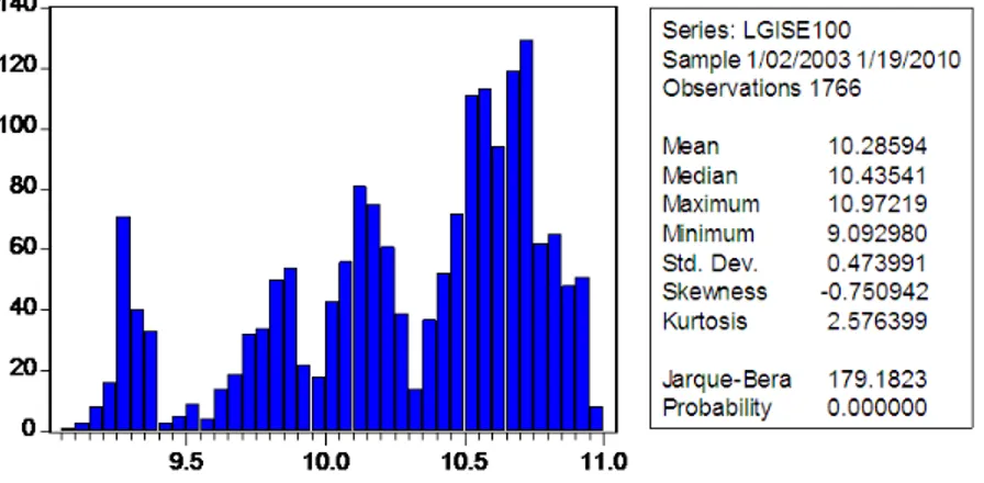
The histogram and descriptive statistics of ISE100 which covers the hundred stock prices is as the following;

Figure 1: Histogram and Descriptive Statistics of log(ISE100)

Section 3.1

Threshold Autoregressive Model (TAR)

&

Continuous Time Threshold Autoregressive Model (CTAR)

As we mention above, threshold autoregressive model (TAR) exhibits the nonlin-earity of time series data. It means that if it is anticipated a change of regime’s presence, regime switching models are used. TAR which is one of the most pop-ular regime switching model seperates from autoregressive model by using two di¤erent slope coe¢ cients such as 1 where the sequence yt 1 > 0 and 2 where

yt 1 0. Then the model is as follows:

yt= 8 > < > : 1yt 1+"1t if yt 1> 0 2yt 1+"2t if yt 1 0 9 > = > ; (1)

Eventhough the sequence yt seems linear when yt 1 > 0 or yt 1 0, the entire

yt is nonlinear. The error terms "1t and "2t have the occurance of two di¤erent

regimes provided. We mean that if yt 1 is positive and close to zero,a negative

value of "1t will cause to change the regime or vice versa. In addition to that if we

assume that the variance of "1t is larger than the variance of "2t, the probability

of switching from positive regime to negative regime is higher than from negative regime to positive regime. On the other hand, if we assume that the two error terms have equal variances then the equation can be written as follows:

yt= 1Ityt 1+ 2(1 I)y_{t 1}+"t (2)

Before studying continuous time threshold autoregressive (CTAR) process, we quickly want to give basic notation of continuous time autoregressive model. We de…ne a zero mean CAR(1) process.

dYt= aYtdt + dWt 1 < t < 1 (3)

Now, we can de…ne continuous time threshold autoregressive model in the paper of Brockwell, Hyndman and Grundwald (1991). We de…ne the CTAR(1) process as follows;

dYt= (a(i)Yt+b(i))dt + (i)dWt ri 1< Xt< ri i = 1; :::; d (4)

where -1 = r0 < r1 < ::: < rl=1; a(i) < 0;each (i) > 0 and b(1); b(2); :::; b(d)

are constants. The threshold are the levels r1; r2; r3; :::; rd 1:If we take d=1, then

Section 3.2

Markov Switching Model

&

Continuous Time Markov Switching Model

In addition to the idea of using probability switching in nonlinear time series analysis which is discussed in Tong (1983), Hamilton (1989) delevopes the Markov switching autoregressive (MSA) model. A time series yt follows an MSA model

if it satis…es yt= 8 > > > > < > > > > : c1+ p X i=1 1;iyt 1+a1t if st=1 c2+ p X i=1 2;iyt 1+a2t if st=2 9 > > > > = > > > > ; (5)

with transition probabilities

p(s_t= 2 _{j st 1}= 1) = w₁; (6)

p(s_t= 1 _{j st 1}= 2) = w₂ (7)

where fa1tg and fa2tg are sequence of iid random variables with mean zero

and …nite variance and are independent each other.Since the states are not di-rectly observable, it is much harder to estimate an MSA model than other mod-els.However, MSA model can easily be generalized to the case of more than two states.

The continuous time Markov switching model which is developed by Bu¤-ington and Elliott (2002) and Guo (2001) comprises of an observed process R = (Rt)t2[0;T ] where Rt= t Z 0 sds+ t Z 0 sdWs; t2 [0; T ] (8)

where (Wt)t2[0;T ] is a standard Brownian Motion , ( t)t2[o;T ] is the time

vary-ing drift and ( t)t2[0;T ] the time varying volatility. The drift process and the

volatility process , taking values in Rn and Rn n, respectively, are continuous time, time homogeneous, irreducible Markov process with d states, adapted to z;independent of W,driven by the state process Y = (Yt)t2[0;T ]. We denote

the possible values of and with (1)_{; :::;} (d) _and (1)_{; :::;} (d)_{, respectively.}

The state process Y, which is a continuous time, time homogeneous, irreducible Markov Process adapted to z; independent of W, with state space f1; :::dg allows for the representations

t= d X k=1 (k)₁ fYt=kg (9) t= d X k=1 (k)₁ fYt=kg: (10)

Section 3.3

Geometric Brownian Motion

GBM which is a type of BM is popular in …nance because of the contribution to the modelling asset price used in the Black-Scholes-Merton option pricing formula. GBM can be de…ned as the follows:

d(S_t) = S_tdt + StdWt (11)

where is called drift, is called volatility, Wt is a normalized BM and St is a

stochastic process.Moreover, both and are constants.

For an arbitrary initial value S0 the equation has the analytic solution

St= S0exp (( 2

2 )t + Wt) (12)

Using transformation and Ito’s formula, we make inference the equation satis…ed by the logarithm of the price. The equation will be as follows:

d(S_t) = (

2

2 )dt + dWt) (13)

The discretized version of the geometric BM is

log St= ( 2

2 ) t + Wt (14)

Let "t= Wt Wt 1;and we know that t = 1:Then the equation can be rewritten

as

log St= 2

2 + "t (15)

Using maximum likelihood method, we can estimate mean and variance of log St: bT=mbT+b 2 T 2 (16) b2T=bs 2 T (17) where mbT = _T1 T X t=1 ( log St) and bs2T = T1 T X t=1 ( log St mbT)2:1

Section 4

The Modi…ed Geometric Brownian Motion and Methodology

As we discussed above, GBM has linear path. In real world, however, the stocks tend to ‡uctuate. In other words, the stocks can change their regimes. Therefore, we want to model another GBM which is nonlinear continuous time model and has been obtained a combination of threshold autoregressive model and Markov switching model. The new model that we compose is as follows:

dSt= 8 > > > > > > > > > > < > > > > > > > > > > : 1Stdt + 1StdW1t (with probability p) if Rt > 0 2Stdt + 2StdW2t (with probability 1-p) 2Stdt + 2StdW3t (with probability q) if Rt< 0 1Stdt + 1StdW4t (with probability 1-q) 9 > > > > > > > > > > = > > > > > > > > > > ; (18)

and a discretized version, we get

4 log St= 8 > > > > > > > > > > < > > > > > > > > > > : ( ₁ 21 2 )dt + 14W1t (with probability p) if Rt> 0 ( ₂ 22 2 )dt + 24W2t (with probability 1-p) ( ₂ 22 2 )dt + 24W3t (with probability q) if Rt < 0 ( ₁ 21 2 )dt + 14W4t (with probability 1-q) 9 > > > > > > > > > > = > > > > > > > > > > ; (19) where Wt = p

t" and " N (0; 1); Rt = log St log St 1 and 1; 2; 1; 2; p; q

To estimate these parameters, we …rstly seperate the dataset into two sub-datasets: one is Rt< 0; the other one is Rt> 0:Then we estimate these

parame-ters as follows; biT=mbiT+b 2 iT 2 (20) b2iT=bs 2 iT (21) wherembiT = _T1 T X t=1 (Rt),bs2iT = T1 T X t=1

(Rt mbiT)2, i = 1 for positive logreturn path

and i = 2 for negative logreturn path.2

To estimate the probabilities p and q, we use Mean Squared Error (MSE) which is a statistical method. The probabilities p and q which minimize MSE of the discretized version of modi…ed GBM are choosen as optimum p and q. MSE is one of many ways to quantify the amount by which an estimator di¤ers from the true value of the quantity being estimated. Suppose the forecast sample is j = T + 1; T + 2; :::; T + h, and denote the actual and forecasted value in period t as yt and ybt, respectively.

The Mean Squared Error statistic is computed as follows:

M SE =1 h T +h X t=T +1 (_byt yt) 2 (22)

Ideally, the MSE will be as small as possible. As the …t of the model improves, the MSE will approach 0. Now, we want to model the stock prices by using two di¤erent models which are discretized GBM and discretized version of modi…ed GBM. Firstly, we assume that stock prices follow GBM de…ned in eq.(11) and and are calculated using eq.(16) and eq.(17). Then, using eq. (14) we estimate stock prices. However, since we have a random variable in the model, we repeat our estimation 50 times to …nd more realistic result . Then we take the mean of 50 MSEs as MSE of discretized GBM. Secondly, we want to reestimate stock 2_{Gourieroux, C. and Jasiak, J. (2001). Financial Econometrics, Princeton University Press, Princeton.}

prices using our discretized version of modi…ed GBM. That means we suppose that the stock prices follow our modi…ed GBM de…ned in eq.(18). We seperate the stock price two parts as positive returns and negative returns. Using eq.(20) and eq.(21), we compute two di¤erent and . It means that there are two di¤erent process as positive and negative.

The processes which has positive path is as follows;

dSt= 1Stdt + 1StdW1t (23)

and the process which has negative path is as follows;

dSt= 2Stdt + 2StdW2t (24)

Now, using eq.(19), we predict stock prices, again. During the prediction, to obtain the stock prices by using the discretized version of modi…ed GBM we should …nd the probabilities which minimize MSE. For this purpose, we …x p = 0. Then q is choosed 0 for the …rst step and will be increased 0.1 for the next step until it reaches 1. For each …xed p and q, MSE is calculated 50 times because of random variable and mean of 50 MSEs is taken as the MSE for these …xed p and q. Furthermore, MSEs are calculated for all combinations of p and q in the same way. After the program calculates MSE for p = q = 1 we have a matrix which includes 121 MSE for all combination of p and q. It searches for minimum MSE and the probabilities p and q which obtain this minimum MSE. However, as we me mentioned above since there exist random variables, we calculate these probabilites p and q 50 times and the means of these probabilities are chosen as optimum probabilites. After …nding the optimal p and q, we again run the program to …nd the MSE for optimum p and q. (The code of Matlab is given in Appendix.) Thus, we have three di¤erent data set now:one is real stock price data, one is the data which is estimated using discretized GBM and the other is

Section 5

Results

As we mentioned above, Mean Squared Errors (MSE) is one of the statistical method which gives us better …t model.We calculate MSE1 for discretized GBM

and MSE2for our discretized version of modi…ed GBM. (The results are attached

to the appendix.)

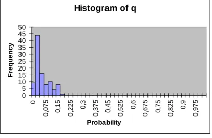
By using classical Geometric Brownian Motion process, we modi…ed a new GBM model using di¤erent data partitions which are seperated two parts as positive and negative paths. Our modi…ed GBM model is obtained by using the probabilities p and q. p is the probability which the stock prices will follow positive process if the return is positive and q is the probability which the stock prices will follow negative process if the return is negative. Figure 3, Figure 4 and Table 1 show us the histograms and statistics of p and q.

Histogram of q 0 5 10 15 20 25 30 35 40 45 50 0 0, 075 _0,15 0, 225 0,3 0, 375 _0,45 0, 525 0,6 0, 675 _0,75 0, 825 0,9 0, 975 Probability Freque ncy Figure 4 p q Mean 0,24802 Mean 0,0413

Standard Error 0,011198286 Standard Error 0,004372307

Median 0,227 Median 0,021 Mode 0,308 Mode 0 Standard Deviation 0,111982861 Standard Deviation 0,043723073

Sample Variance 0,012540161 Sample Variance 0,001911707

Kurtosis 2,943610 Kurtosis 2,856139 Skewness 0,190989 Skewness 1,061910 Rang e 0,582 Ran ge 0,156 Minimum 0,006 Minimum 0 Maximum 0,588 Maximum 0,156 Sum 24,802 Sum 4,13 Count 100 Cou nt 100

Table 1: Statistics of p and q

The mean values of p and q, are 0.248 and 0.041, respectively. In addition to that, skewness of p and q are 0.191 and 1.062, respectively. It means that both of the probabilities have right skewed. In other words, they have relatively few high values. When we look at these values, we obviously realize that the probabilities p and q take low values. That means if the stock prices have positive returns today, they will follow negative process tomorrow and if the stock prices have negative returns, they follow positive process. Addionally, according to the

values of probabilites it can be said that p which is the probability of following negative process during negative logreturn is lower than q which is the probability of following positive during the positive logreturns. As a result, we can say that positive return pursue negative process and negative return pursue positive process.

Section 7

Conclusions and Future Work

The aim of this study is to develop a discretized version of modi…ed nonlinear GBM. As we mentioned above, our discretized version of modi…ed GBM is formed of two di¤erent process as positive return path and negative return path. If logreturn of stock prices is positive at time t, then the process follows positive path with probability p or negative path with probability 1 pat time t + 1. On the other hand, if logreturn of stock prices is negative at time t, then the process follows negative path with probability q or positive path with probability 1 q at time t + 1. When we look at the probabilities p and q which minimize MSE, we clearly realize that stock prices follow the process of negative logreturn with higher probability at time t + 1 if the logreturn is positive at time t, vice versa. This may be attributable to the expectation of the investors which changes by the movements of stock prices. In other words, if the stock prices increase then the investors expect that the prices will decrease, begin to sell their stocks and the stock prices will reduce, vice versa.

So far, we compose a discrete version of nonlinear GBM which is designed to give better than GBM according to MSE. To develop this study, we will compare our model and another nonlinear GBM which is developed by a barrier strategy. It means that, we will try to show that our model gives better …t than this GBM model according to MSE. On the other hand, we may show that modi…ed GBM gives us a better pricing results than GBM by using option pricing model. Hence, we require to develop this study to show that modi…ed GBM gives better prediction than GBM for option price model. On the other hand, we can improve our modi…ed GBM model by using stochastic volatility models.

References

1. Aingworth, D. D., Das, S. R. and Motwani, R. (2006). A Simple Approach for Pricing Equity Options with Markov Switching State Variables. Quantitative Finance, 6: 95-105.

2. Alexander, C. (2008). Market Risk Analysis I: Quantitative Methods in Finance.John Wiley & Sons Ltd, Chichester.

3. Brockwell, P. J., Chadraa, E. and Lindner, A. (2006). Continuous-Time Garch Processes. The Annals of Applied Probability, 16: 790-826.

4. Brockwell, P. J., Hyndman, R. J. and Grunwald, G. K. (1991). Continuous Time Threshold Autoreressive Models. Statistica Sinica, 1: 401-410.

5. Brooks, C. (2008). Introductory Econometrics for Finance. Cambridge University Press, Cambridge.

6. Bu¢ ngton, J. and Elliott, R. J. (2002). American Option with Regime Switching. Journal of Theoretical and Applied Finance, 5: 497-514.

7. Campbell, J. Y., Lo, A. W. and MacKinlay, A. C. (1997). The Econometrics of Fi-nancial Markets. Princeton University Press, Princeton and New Jersey.

8. Chourdakis, K. (2002). Continuous Time Regime Switching Models and Applications in Estimating Processes with Stochastic Volatility and Jumps. University of London Queen MAry Economics Working Paper No. 464.

9. Elliott, R. J.,Krishnamurthy, V. and Sass, J. (2008). Moment based regression algo-rithms for drift and volatility estimation in continuous-time Markov switching models. Econometrics Journal, 11: 244-270.

10. Enders, W. (2004). Applied Econometric Time Series, 2nd edition. John Wiley & Sons, Hoboken.

11. Gallant, A. R. and Tauchen, G. (1997). Estimation of Continuous-Time Models for Stock Returns and Interest Rates. Macroeconomic Dynamics, 1: 135-168.

12. Gerber, H. U. and Shiu, S. W. (2003). Geometric Brownian Motion Models for Assets and Liabilities: From Pension Funding to Optimal Dividends. North American Acturial Journal, 7: 37-56

13. Gourieroux, C. and Jasiak, J. (2001). Financial Econometrics. Princeton University Press, Princeton and Oxford.

14. Gray, F. G. (1996). Modeling the Conditional Distribution of Interest Rates as a Regime-Switching Process. Journal of Financial Economics, 42: 27-62.

15. Guidolin, M. and Timmermann, A. (2006). An Econometric Model of Nonlinear dy-namics in the Joint Distribution of Stock and Bond Returns. Journal of applied Econo-metrics, 21: 1-22.

16. Guo, X. (2001). An Explicit Solution to an Optimal Stopping Problem with Regime Switching. Journal of Applied Probability, 38: 464-481.

17. Hahn, M., Frühwirth-Schnatter, S. and Sass, J. (2007). Markov Chain Monte Carlo Methods for Parameter Estimation in Multidimensional Continuous Time Markov Switching Models. Journal of Financial Econometrics, 8: 88-121.

18. Hahn, M. and Sass, J. (2009). Parameter Estimation in Continuous Time Markov Switching Models: A Semi-Continuous Markov Chain Monte Carlo Approach. Bayesian Analysis, 4: 63-84.

19. Hamilton, J. D. (1994). Time Series Analysis. Princeton University Press, Princeton and New Jersey.

20. Hamilton, J. D. and Susmel, R. (1994). Autoregressive Conditional Heteroskedasticity and Changes in Regime. Journal of Econometrics, 64: 307-333.

21. Hansen, B. E. (1997). Inference in TAR Models. Forthcoming in Studies in Nonlinear Dynamics and Econometrics.

22. Hardy, M. R. (2001). A Regime-Switching Model of Long-Term Stock Returns. North American Actuarial Journal, 5, 41-53.

23. Ismail, M. T. and Isa, Z. (2008). Identifying Regime Shifts in Malaysian Sstock Market Returns. International Research Journal of Finance and Economics, 14: 44-57

24. Klüppelberg, C., Lindner A. M. and Maller, R. A. (2004). A Continuous Time GARCH Process Driven by a L·evy Process: Stationarity and Second Order Behaviour. Journal of Applied Probability, 41:601-622.

25. Maheu, J. M. and McCurdy, T. H. (2000). Identify Bull and Bear Markets in Stock Returns. Journal of Business and Economic Statistics, 18: 100-112.

26. Nishiyama, K. (1998). Some Evidence on Regime Shifts in International Stock Markets. Managerial Finance, 24: 30-55.

27. Norden, S. V. and Schaller, H. (1997). Regime Switching in Stock Market Returns. Applied Financial Economics, 7: 177-191.

28. Shreve, S. E. (2004). Stochastic Calculus for Finance II- Continuous Time Models. Springer, New York.

29. Tsay, R. S. (2005). Analysis of Financial Time Series, 2nd edition. John Wiley & Sons, New Jersey.

30. Tong, H. and Yeung, I. (1991). Threshold Autoregressive Modelling in Continuous Time. Statistica Sinica, 1: 411-430.

31. Yin, G., Wang, J. W., Zhang, Q. and Liu, Y. J. (2006). Stochastic Optimization Al-gorithms for Pricing American Put Options under Regime-Switching Models. Journal of Optimization Thoery and Applications, 131: 37-52.

Appendix

i.Matlab Codes x=xlsread(’asset’); results=[]; t=length(x(:,1)); for row=1:100 N =50; M=50; y=[]; z=[]; h=[]; l=[]; k1=[]; k2=[]; f=[]; ms2=[]; mse2=[]; mmse2=[]; ms12=[]; mse12=[]; y=log(x(:,row)); ab=isnan(x(:,row)); to=sum(ab); ko=t-to; dif=(-y(1:t-1)+y(2:t))’; m = mean(dif(1:ko-1));

for i=1:t-1 k(i)=(dif(i)-m)^2; end varyans = mean(k(1:ko-1)); nu = m+varyans/2; dt=1; z(1)=y(1); z(2)=y(2); for j=1:N e=normrnd(0,1,1,t); for i=3:ko z(i)=z(i-1)+(nu-varyans/2)*dt+sqrt(varyans)*sqrt(dt)*e(i); ms1(i)=(z(i)-y(i))^2; end mse1(j)=mean(ms1); end mmse1=mean(mse1); m=1;

n=1; for i=2:ko if y(i)>=y(i-1) h(m)=y(i)-y(i-1); m=m+1; else l(n)=y(i)-y(i-1); n=n+1; end end m1=mean(h); for i=1:m-1 k1(i)=(h(i)-m1)^2; end varyans1=mean(k1); nu1=m1+varyans1/2; m2=mean(l); for i=1:n-1 k2(i)=(l(i)-m2)^2; end varyans2=mean(k2); nu2=m2+varyans2/2; f(1)=y(1); f(2)=y(2); d=1; for dr=1:M for r=0:0.1:1 for rr=0:0.1:1

for j=1:N u=rand(1,t); e1=normrnd(0,1,1,t); e2=normrnd(0,1,1,t); e3=normrnd(0,1,1,t); e4=normrnd(0,1,1,t); for i=2:ko-1 if f(i)>f(i-1) if r>=u(i) f(i+1)=f(i)+(nu1-varyans1/2)*dt+sqrt(varyans1)*sqrt(dt)*e1(i); else f(i+1)=f(i)+(nu2-varyans2/2)*dt+sqrt(varyans2)*sqrt(dt)*e2(i); end else if rr>=u(i) f(i+1)=f(i)+(nu2-varyans2/2)*dt+sqrt(varyans2)*sqrt(dt)*e3(i); else f(i+1)=f(i)+(nu1-varyans1/2)*dt+sqrt(varyans1)*sqrt(dt)*e4(i);

end end ms2(i)=(f(i)-y(i))^2; end mse2(j)=mean(ms2); end mmse2(d)=mean(mse2); d=d+1; end end [mmse22,ii]=min(mmse2); kt=‡oor(ii/11); if ii-kt*11==0 r1=(kt-1)*0.1; rr1=1; else r1=kt*0.1; rr1=(ii-kt*11-1)*0.1; end prob(dr,1)=r1; prob(dr,2)=rr1; r1=0; rr1=0; d=1; end r12=mean(prob(:,1)); rr12=mean(prob(:,2)); for j=1:N

u=rand(1,t); e1=normrnd(0,1,1,t); e2=normrnd(0,1,1,t); e3=normrnd(0,1,1,t); e4=normrnd(0,1,1,t); for i=2:ko-1 if f(i)>f(i-1) if r12>=u(i) f(i+1)=f(i)+(nu1-varyans1/2)*dt+sqrt(varyans1)*sqrt(dt)*e1(i); else f(i+1)=f(i)+(nu2-varyans2/2)*dt+sqrt(varyans2)*sqrt(dt)*e2(i); end else if rr12>=u(i) f(i+1)=f(i)+(nu2-varyans2/2)*dt+sqrt(varyans2)*sqrt(dt)*e3(i); else f(i+1)=f(i)+(nu1-varyans1/2)*dt+sqrt(varyans1)*sqrt(dt)*e4(i); end end ms12(i)=(f(i)-y(i))^2; end mse12(j)=mean(ms12); end mmse12=mean(mse12); results(row,1)=r12; results(row,2)=rr12; results(row,3)=mmse1; results(row,4)=mmse12;

ii. Estimation Outputs

Stocks p q mse1 mse2

adana 0,304 0,004 0,980 0,435 aefes 0,356 0,156 0,543 0,453 afyon 0,204 0,004 1,249 0,790 agyo 0,400 0,000 1,134 0,743 akbnk 0,202 0,002 1,016 0,631 akcns 0,204 0,004 1,013 0,478 akenr 0,210 0,010 0,716 0,327 akgrt 0,280 0,080 1,058 0,751 aksa 0,104 0,004 0,504 0,221 alark 0,210 0,010 0,536 0,532 albrk 0,030 0,030 0,709 0,086 alkim 0,208 0,008 0,889 0,384 anhyt 0,316 0,116 1,825 0,900 angsr 0,404 0,004 1,200 0,534 arclk 0,138 0,038 0,988 0,708 asels 0,182 0,068 1,050 0,639 asyab 0,150 0,050 0,767 0,383 aygaz 0,166 0,066 0,460 0,320 bagfs 0,340 0,140 0,821 0,667 banvt 0,224 0,024 0,596 0,577 bimas 0,246 0,046 0,385 0,250 bjkas 0,006 0,006 2,091 1,227 ccola 0,214 0,014 7,337 0,186 clebi 0,120 0,020 0,955 0,560 deva 0,308 0,008 1,566 1,046 dgzte 0,040 0,016 1,328 0,720 doas 0,130 0,030 0,884 0,389 dohol 0,360 0,060 1,198 0,685 dyhol 0,230 0,064 1,824 0,995 ecilc 0,400 0,000 0,939 0,625 eczyt 0,332 0,132 0,662 0,421 eggub 0,208 0,008 1,114 0,633 egser 0,212 0,012 2,134 0,842 enkai 0,266 0,076 9,681 6,302 eregli 0,300 0,000 1,002 0,518 fener 0,464 0,092 0,712 0,360 fenis 0,370 0,070 1,433 0,672 ffkrl 0,356 0,056 2,026 1,036 finbn 0,400 0,000 1,483 0,799 fortis 0,308 0,008 1,778 0,847 froto 0,308 0,108 0,857 0,631 garanti 0,334 0,134 1,054 0,745 golds 0,252 0,052 1,325 0,693 gsdho 0,212 0,012 1,220 0,554 gubrf 0,304 0,004 1,956 0,854 gyho 0,308 0,008 1,281 0,716 halkbnk 0,112 0,012 0,950 0,174 hurgz 0,198 0,098 1,037 1,068 iheva 0,216 0,016 1,942 0,988 ihlas 0,218 0,018 1,136 0,702 isctr 0,206 0,006 1,251 0,482

isfin 0,492 0,092 2,267 1,677 isgyo 0,300 0,000 1,216 0,716 izmdc 0,330 0,130 0,821 0,898 karsn 0,120 0,020 0,928 0,743 kchol 0,186 0,086 0,571 0,671 kipa 0,312 0,012 0,979 0,579 koza 0,216 0,016 1,841 0,964 krdmd 0,588 0,088 1,905 1,458 marti 0,312 0,084 1,379 0,993 nthol 0,402 0,002 1,295 1,078 nttur 0,302 0,020 1,302 0,964 otkar 0,334 0,134 0,812 0,483 pegyo 0,430 0,130 1,421 1,047 petk 0,202 0,004 0,731 0,492 petum 0,436 0,136 0,694 0,635 pnsut 0,296 0,096 1,500 0,714 prkte 0,142 0,010 1,285 0,739 ptofs 0,190 0,018 0,720 0,452 pysas 0,122 0,022 0,620 0,435 sahol 0,200 0,000 0,734 0,667 sasa 0,314 0,014 0,752 0,607 seles 0,016 0,016 0,205 0,148 sise 0,382 0,122 1,078 0,596 skbnk 0,308 0,008 1,767 1,054 sngyo 0,016 0,116 5,386 0,270 tatks 0,144 0,030 0,606 0,480 tavhl 0,118 0,018 0,687 0,188 tcell 0,202 0,002 0,635 0,281 tebank 0,436 0,136 1,658 0,929 tekfn 0,356 0,056 2,044 1,077 thyoa 0,164 0,036 0,870 0,342 tire 0,326 0,026 1,038 0,361 tkstl 0,124 0,024 0,638 0,194 toaso 0,200 0,000 1,278 0,631 tprs 0,246 0,046 3,130 2,235 trcas 0,300 0,000 0,659 0,405 trkcm 0,400 0,000 1,655 0,916 tskm 0,328 0,028 0,601 0,263 tspor 0,112 0,016 0,453 0,050 ttkm 0,204 0,010 0,609 0,503 ttrak 0,294 0,094 0,791 0,448 tupras 0,244 0,044 1,936 1,195 vakifbnk 0,108 0,008 0,641 0,286 vanet 0,238 0,038 0,989 0,503 vesbe 0,146 0,044 0,510 0,338 vestel 0,134 0,034 0,829 0,536 ykbnk 0,204 0,004 0,883 0,626 yksrg 0,126 0,026 1,431 0,508 zoren 0,130 0,030 0,740 0,354