Computational analysis of the search based cuts on the multidimensional 0-1 knapsack problem

SEARCH BASED CUTS ON THE

MULTIDIMENSIONAL 0-1 KNAPSACK PROBLEM

A THESIS

SUBMITTED TO THE DEPARTMENT OF INDUSTRIAL ENGINEERING

AND THE INSTITUTE OF ENGINEERING AND SCIENCES OF BILKENT UNIVERSITY

IN PARTIAL FULFILLMENT OF THE REQUIREMENTS FOR THE DEGREE OF

MASTER OF SCIENCE

by Duygu Pekbey September 2003

Assoc. Prof. Osman Oğuz (Principal Advisor)

I certify that I have read this thesis and that in my opinion it is fully adequate, in scope and in quality, as a thesis for the degree of Master of Science.

Assoc. Prof. Mustafa Ç. Pınar

I certify that I have read this thesis and that in my opinion it is fully adequate, in scope and in quality, as a thesis for the degree of Master of Science.

Asst. Prof. Bahar Y. Kara

Approved for the Institute of Engineering and Sciences:

Prof. Mehmet Baray

COMPUTATIONAL ANALYSIS OF THE SEARCH BASED CUTS ON THE MULTIDIMENSIONAL 0-1 KNAPSACK PROBLEM

Duygu Pekbey

M. S. in Industrial Engineering Supervisor: Assoc. Prof. Osman Oğuz

September 2003

In this thesis, the potential use of a recently proposed cut (the search based cut) for 0-1 programming problems by Oguz (2002) is analyzed. For this purpose, the search based cuts and a new algorithm based on the search based cuts are applied to multidimensional 0-1 knapsack problems from the literature as well as randomly generated multidimensional 0-1 knapsack problems. The results are compared with the implementation of CPLEX v8.1 in MIP mode and the results reported.

Key Words: 0-1 Integer Programming, Multidimensional 0-1 Knapsack Problem

ARAŞTIRMA TABANLI KESMELERİN ÇOK BOYUTLU 0-1 SIRT ÇANTASI PROBLEMLERİ ÜZERİNDE HESAPSAL ANALİZİ

Duygu Pekbey

Endüstri Mühendisliği Yüksek Lisans Tez Yöneticisi: Doç. Dr. Osman Oğuz

Eylül 2003

Bu çalışmada, yakın zamanda 0-1 programlama problemleri için Oguz (2002) tarafından önerilen bir kesmenin (araştırma tabanlı kesme) potansiyel faydası analiz edilmektedir. Bu amaçla, araştırma tabanlı kesmeler ve bunlar üzerine kurulan yeni bir algoritma literatürdeki çok boyutlu 0-1 sırt çantası problemlerine ve rastlantısal olarak oluşturulan çok boyutlu 0-1 sırt çantası problemlerine uygulanmaktadır. Sonuçlar CPLEX v8.1' in MIP biçimindeki uygulaması ve literatürdeki sonuçlarla karşılaştırılmaktadır.

Anahtar Kelimeler: 0-1 tamsayılı programlama, çok boyutlu 0-1 sırt çantası problemleri

I would like to express my sincere gratitude to Assoc. Prof. Osman Oğuz for his guidance, attention and patience throughout our study.

I wish to express my thanks to the readers Assoc. Prof. Mustafa Ç. Pınar and Asst. Prof. Bahar Y. Kara for their effort, kindness and time.

I would like to thank Aykut Özsoy, Güneş Erdoğan, Ünal Akmeşe, Çağatay Kepek, Hakan Ümit and Pınar Tan for their assistance, support and friendship during the graduate study. I am also very thankful to all Industrial Engineering Department staff.

I am grateful to Çağdaş Yavuz and Karim Saadaoui for their support and friendship.

Finally, I would like to thank my family, and especially my sister for her invaluable support and love.

1 Introduction ...1

2 Literature Review ...4

3 The Partitioning Algorithm ...17

3.1 Description of the Search Based Cuts ...17

3.2 Partitioning the Problem ...19

3.3 An example ...22

3.4 Computational Experimentation and Results ...26

3.5 One Step Partitioning Algorithm ...29

4 Computational Analysis of the Search Based Cuts ...32

4.1 Computational Analysis of the Search Based Cuts Applied to the Multidimensional 0-1 Knapsack Problem ...32

4.2 Computational Analysis of the Search Based Cuts Applied to the Set Covering Problem ...39

5 Application of the Partitioning Algorithm to the Multidimensional 0-1 Knapsack Problem ...45

5.1 Problem Generation ...45

5.2 Computational Results ...46

6 Conclusion ...57

LIST OF FIGURES

4-1a: Absolute reduction in the objective value per cut as n increases ...35 4-1b: Absolute reduction in the objective value per cut as m increases ...38 4-2: Absolute increase in the objective value per cut as n increases ...42

LIST OF TABLES

3-4: Computational results for standard test problems (Shih (1979)) ...27

4-1a: Computational results for m=5, α=0.5 and n=100 OR-lib. instances ...33

4-1b: Computational results for m=5, α=0.5 and n=250 OR-lib. instances ...33

4-1c: Computational results for m=5, α=0.5 and n=500 OR-lib. instances ...34

4-1d: Average value of absolute reduction in the objective value per cut for m=5, α=0.5 ...35

4-1e: Computational results for n=100, α=0.5 and m=5 OR-lib. instances ...36

4-1f: Computational results for n=100, α=0.5 and m=10 OR-lib. instances ..36

4-1g: Computational results for n=100, α=0.5 and m=30 OR-lib. instances .37 4-1h: Average value of absolute reduction in the objective value per cut for n=100, α=0.5 ...37

4-2a: Computational results for m=5 and n=100 set covering problems ...40

4-2b: Computational results for m=5 and n=150 set covering problems ...40

4-2c: Computational results for m=5 and n=200 set covering problems ...40

4-2d: Average value of absolute increase in the objective value per cut for m=5 ...41

4-2g: Average value of absolute increase in the objective value per cut for n=100 ...43 5-2a: Computational results for n=500 and m=10 OR-library instances ...48 5-2b: Computational results for n=1000 and m=10 randomly generated instances ...49 5-2c: Computational results for n=2000 and m=10 randomly generated instances ...50 5-2d: Comparison of one step partitioning algorithm with Cplex and genetic algorithm of Chu and Beasley ...52 5-2e: Comparison of one step partitioning algorithm with Cplex for n=1000 randomly generated instances ...53 5-2f: Comparison of one step partitioning algorithm with Cplex for n=2000 randomly generated instances ...54 5-2g: Computational results of the problems for which the experiment was repeated ...56

Introduction

In this thesis, a computational study on the potential use of a recently proposed cut for 0-1 programming problems by Oguz (2002) is presented. The cut is of a general type, and can be used for almost any 0-1 integer programming problem. We have chosen to focus on and limit the scope of the study to the multidimensional 0-1 knapsack problems for a couple of reasons. Firstly, extending the scope to cover several types of combinatorial optimization problems would require development of much more sophisticated and expert programming skills and effort, and longer time. Secondly, a wide array of test problems and computational results on this specific problem already exist in the literature and it is easier to carry out comparative analysis with this problem.

In this study, in order to analyze the potential use of the search based cuts (see Oguz (2002)), we have applied them to 60 multidimensional 0-1 knapsack problems (0-1 MDKP) from the literature as well as 25 randomly generated set covering problems. In addition, in order to check the efficiency of the partitioning algorithm-a new algorithm based on the search based cuts-, we have made computational experiments with 30 small-sized 0-1 MDKP from the literature (Shih (1979)) as well as randomly generated 0-1 MDKP with different numbers of variables and different numbers of constraints.

In order to reduce the computational time and effort required by the partitioning algorithm, we presented a modification of the partitioning

algorithm which we named "one step partitioning algorithm" and made computational experiments with 60 randomly generated large sized 0-1 MDKP as well as 30 large-sized 0-1 MDKP from the literature (Chu and Beasley (1998)). We compared our results with the implementation of CPLEX v8.1 in MIP mode and the results reported by Chu and Beasley (1998).

The remaining part of this thesis is organized as follows: After introducing the multidimensional 0-1 knapsack problem briefly, we present a comprehensive survey of the work done for it in the literature in the next chapter. In chapter 3, the "search based cuts" and the "partitioning algorithm" are discussed. In chapter 4, computational analysis of the search based cuts is presented and in chapter 5, computational results of the application of one step partitioning algorithm to the large-sized 0-1 MDKP are reported. Finally, some conclusions and remarks for future works are given in chapter 5.

The Multidimensional 0-1 Knapsack Problem

The multidimensional 0-1 knapsack problem (0-1 MDKP) is an important combinatorial optimization problem which is widely studied in the literature and can be employed to formulate many practical problems such as capital budgeting or resource allocation. As an example, think that there are n projects with known profits cj and project j consumes aij units from resource

i given bi as the capacity of resource i. The goal is to select a group of

projects to allocate resources in such a way that the profit is maximized and the capacity of any resource is not exceeded. Other applications of the multidimensional 0-1 knapsack problem include cutting stock problems

(Gilmore and Gomory (1966)), cargo loading (Shih (1979)) and allocating processors and databases in distributed systems (Gavish and Pirkul (1982)). The 0-1 MDKP can be considered as a general 0-1 integer programming problem with non-negative coefficients and can be formulated as follows:

n maximize

∑

∑

where aij ≥ 0 for i = 1, . . . , m; j = 1, . . . , n; bi > 0 for i = 1, . . . , m and

cj > 0 for j = 1, . . .,n.

In addition, for the problem to be meaningful, the following must be true:

n

bi <

∑

j=1

aij < bi for i = 1, . . . , m ; j = 1, . . . , n (otherwise xj will be fixed to zero).

If m = 1, the problem is the standard knapsack problem which is proven to be NP-complete(see Garey and Johnson (1979)). Since the standard knapsack problem is NP-complete, the multidimensional 0-1 knapsack problem is also NP-complete.

Literature Review

Most of the research on knapsack problems deals with the standard knapsack problem (m = 1) and a good review of exact and heuristic algorithms for the standard knapsack problem is given by Martello and Toth (1990). Below we review exact and heuristic algorithms designed to solve the multidimensional 0-1 knapsack problem (0-1 MDKP).

Gilmore and Gomory (1966), and Nemhauser and Ullmann(1969) developed dynamic programming based methods to solve the 0-1 MDKP. However, they were not able to solve large instances. Nemhauser and Ullmann(1969) reported that for the problems that they had solved the number of variables was at most 50. Weingartner (1967), and Weingartner and Ness (1967) also developed dynamic programming based methods to solve the 0-1 MDKP and Cabot (1970) developed an enumeration algorithm based on Fourier-Motzkin elimination.

Soyster, Lev, and Slivka (1978) developed an algorithm for solving zero-one integer programs with many variables and few constraints. In their algorithm, sub-problems were generated from the linear programming relaxation and solved through implicit enumeration. The variables in these sub-problems corresponded to the fractional variables obtained in the linear program. The number of variables in the sub-problems is much less than the number of variables in the original zero-one integer program because the number of fractional variables in the linear program is bounded by the number of constraints in the linear program.

Senju and Toyoda (1968) proposed a dual gradient method that starts with a possibly infeasible initial solution (all decision variables set to 1) and achieves feasibility by dropping the non-rewarding variables one by one, while following an effective gradient path.

Zanakis (1977) compared three heuristic algorithms for the 0-1 MDKP from Hillier (1969); Kochenberger, McCarl, and Wymann (1974); Senju and Toyoda(1968) and reported that none was found to dominate the others computationally.

In order to apply the greedy method for standard knapsack problem where items are picked from the top of a list sorted in decreasing order on cj/aj

(Martello and Toth (1987)) to the 0-1 MDKP, Toyoda (1975) proposed a new measurement called aggregate resource consumption. He developed a primal gradient method that improves the initial feasible solution (all decision variables set to zero) by incrementing the value of the decision variable with the steepest effective gradient. Using the basic idea behind Toyoda’s primal gradient method, Loulou and Michaelides (1979) developed a greedy-like algorithm that expands the initial feasible solution by including the decision variable with the maximum pseudo-utility. The pseudo-utility is defined as uj = cj/vj , where vj is the penalty factor of variable j , which

depends on the resource coefficients aij and can be defined in several ways.

They tested this method on small-sized randomly generated problems as well as some larger real-world problems and showed that the average deviation from optimum ranged from 0.26% to 1.08% for smaller problems and up to 14% for larger problems.

Balas and Martin (1980) presented a heuristic algorithm for the 0-1 MDKP which utilizes linear programming by relaxing the integrality constraints xj Є

{0, 1} to 0 ≤ xj ≤ 1. The fractional xj are then set to 0 or 1 according to a

heuristic which maintains feasibility.

Shih (1979) proposed a branch and bound algorithm for the 0-1 MDKP. In this algorithm, estimation of an upper bound for a node was made by solving m single constraint knapsack problems with the same objective function. An optimal fractional solution (Dantzig (1957)) was found for each of the m single constraint knapsack problems separately. To find optimal fractional solution one must include as much as possible of each item in the order of decreasing cj/aij to the knapsack i until the constraint i is satisfied exactly as

an equation. Minimum of the objective function values associated with each optimal fractional solution was chosen as the upper bound for that node. The node selected for next branching would be the end node whose upper bound is maximum of all end nodes and where the solution associated with such an upper bound is infeasible(if solution is feasible it is also an optimal solution). The branching variable would be the one whose cj/aij ratio is

minimum of all non-zero free variables in this infeasible solution.

Shih solved thirty 5-constraint knapsack problems with 30-90 variables (we also used this data to test our first algorithm) and reported that his algorithm is faster than original Balas and improved Balas additive algorithms (Balas (1965)) with respect to the total as well as the individual solution times. Using Senju and Toyoda 's dual gradient algorithm and Everett (1963) 's generalized lagrange multipliers approach, Magazine and Oguz (1984) proposed another heuristic that moves from the initial infeasible solution (all variables set to 1) towards a feasible solution by following a direction which reduces the aggregate weighted infeasibility among all resource constraints. Their algorithm was tested on randomly generated problems with sizes from

m = 20 to 1,000 and n = 20 to 1,000, and its computational efficiency is compared with two other well-known heuristics: the primal heuristic of Kochenberger, McCarl, and Wymann (1974) (1) and the dual approach of Senju and Toyoda (1968)(2). They reported that, in terms of solution quality, (1) produced slightly better results than their heuristic and their heuristic was superior to (2). Their heuristic and (2) were much better than (1) in terms of computation time.

Fox and Scudder (1985) presented a heuristic based on starting from setting all variables to zero(one) and successively choosing variables to set to one(zero). They reported results for randomly generated test problems with sizes up to m = 100 and n = 100, and with cj = 1 and aij = 0 or 1.

Gavish and Pirkul (1985) proposed another branch and bound algorithm in which they used tighter upper bounds obtained with relaxation techniques such as lagrangean, surrogate and composite relaxations. They tried to evaluate the quality of the bounds generated by these different relaxations and showed that the composite relaxation (which used a subgradient optimization procedure to determine the multipliers) yielded the best bounds overall, but needed extra computational effort. They developed new algorithms for obtaining surrogate bounds and suggested rules for reducing the problem size. They tested their algorithm on a set of randomly generated problems with sizes up to m = 5 and n = 200 and reported that it is faster than the branch and bound algorithm of Shih (1979). They showed that if their algorithm is used as a heuristic by terminating it before the tree search is completed, then it is superior to the heuristic developed by Loulou and Michaelides (1979).

using the dual variables (known as the surrogate multipliers) obtained from the linear programming relaxation of the 0-1 MDKP. He then obtained a feasible solution to this problem using a greedy algorithm based on the ordering of the profit to weight ratios. This ratio was defined as,

m

cj /

∑

i=1

where wi is the surrogate multiplier for constraint i. Surrogate multipliers

were determined using a descent procedure. He reported that the algorithm was considerably better than the heuristic of Loulou and Michaelides (1979) and similar to the pivot and complement heuristic of Balas and Martin (1980) in terms of solution quality.

Lee and Guignard (1988) presented a heuristic that combined Toyoda’s primal heuristic (1975) with variable fixing, linear programming and a complementing procedure from Balas and Martin (1980). Computational experiments were done with standard test problems and randomly generated problems with sizes up to m = 20 and n = 200. They reported that their heuristic produced better results than Toyoda (1975) and Magazine and Oguz (1984), but is out-performed by Balas and Martin (1980).

Drexl (1988) presented a heuristic based upon simulated annealing. They made experiments with 57 standard 0-1 MDKP test problems from the literature and found optimal solutions for 25 of these problems.

Volgenant and Zoon (1990) extended Magazine and Oguz’s heuristic in two ways: (1) in each step, not one, but more multiplier values are computed simultaneously, and (2) at the end the upper bound is sharpened by changing some multiplier values. They showed that these extensions yielded an

improvement, on average, at the cost of only a modest amount of extra computing time.

Crama and Mazzola (1994) showed that although the bounds obtained with relaxation techniques such as lagrangean, surrogate, or composite relaxations, are stronger than the bounds obtained from the linear programming relaxation, the improvement in the bound that can be achieved using these relaxations is limited. In fact, the improvement in the quality of the bounds using any of these relaxations cannot exceed the magnitude of the largest coefficient in the objective function.

There are a few number of papers considering a statistical-asymptotic analysis of the 0-1 MDKP. Schilling (1990) presented an asymptotic analysis and computed the asymptotic objective function value of a particular m constraint, n variable 0-1 random integer programming problem as n increases and m remaining fixed. In this analysis, the aij 's and cj 's were

uniformly and independently distributed over the unit interval and bi = 1.

Szkatula (1994) generalized that analysis to the case where the bi were not

restricted to be one (see also Szkatula (1997)). A statistical analysis was presented by Fontanari (1995) in which he investigated the dependence of the multidimensional knapsack objective function on the knapsack capacities and on the number of capacity constraints, in the case when all n objects were assigned the same profit value and the aij 's were uniformly distributed

over the unit interval. A rigorous upper bound to the optimal profit was obtained employing the annealed approximation and then compared with the exact value obtained through a lagrangean relaxation method.

Freville and Plateau (1994) presented an efficient preprocessing procedure for the 0-1 MDKP based on their previous work ((Freville and Plateau

(1986)) and they also proposed a heuristic for the bidimensional knapsack problem (Freville and Plateau (1997)).

Dammeyer and Voss (1993) proposed a tabu search heuristic for the 0-1 MDKP based on reverse elimination method. They made computational experiments with 57 standard test problems from the literature and reported that they found optimal solutions for 41 of these problems.

Aboudi and Jörnsten (1994) combined tabu search with the pivot and complement heuristic of Balas and Martin (1980) in a heuristic for general zero-one integer programming. They made computational experiments with 57 standard test problems and found optimal solutions for 49 of these problems.

Løkketangen, Jörnsten, and Storøy (1994) presented a tabu search heuristic within a pivot and complement framework and gave computational results for the same set of test problems. They found optimal solutions for 39 of these problems.

Glover and Kochenberger (1996) presented a heuristic based on tabu search. They employed a flexible memory structure that integrates recency and frequency information keyed to “critical events” in the search process. Their method was enhanced by a strategic oscillation scheme that alternates between constructive (current solution feasible) and destructive (current solution infeasible) phases. They define a “critical event” as the last feasible solution found after a transition between phases. They found optimal solutions for each of 57 standard test problems from the literature.

Løkketangen and Glover (1996) presented a heuristic based on probabilistic tabu search for solving general zero-one mixed-integer programming

problems. They made computational experiments with 18 standard test problems and found optimal solutions for 13 of these problems.

Løkketangen and Glover (1997) presented a tabu search heuristic for solving general zero-one mixed-integer programming problems. They made experiments with 57 standard test problems and found optimal solutions for 54 of these problems.

Hanafi and Freville (1997) presented an efficient tabu search approach for the 0-1 MDKP, a heuristic algorithm strongly related to the work of Glover and Kochenberger (1996). They described a new approach to tabu search based on strategic oscillation and surrogate constraint information that provides a balance between intensification and diversification strategies. New rules needed to control the oscillation process were given for the 0-1 MDKP. They tested their approach on 54 instances from Freville and Plateau (1986) and 24 instances from Glover and Kochenberger(1996). Optimal solutions were obtained for the first set of problems and better results than Glover and Kochenberger (1996) were reported for the second set.

Khuri, Bäck, and Heitkötter (1994) presented a genetic algorithm to solve the 0-1 MDKP. In their algorithm, infeasible solutions were allowed to participate in the search and a simple fitness function that uses a graded penalty term was used. They applied their algorithm on 9 test problems taken from the literature and reported moderate results. The problem sizes ranged from 15 objects to 105 and from 2 to 30 knapsacks.

Thiel and Voss (1994) suggested an algorithm for the 0-1 MDKP by combining a genetic algorithm implementation with tabu search. They tested their heuristic on a set of standard test problems, but the results were not

computationally competitive with the results obtained using other heuristic methods.

Hoff, Løkketangen, and Mittet (1996) presented a genetic algorithm for the 0-1 MDKP in which only feasible solutions were allowed. They found optimal solutions for 56 of the 57 test instances from the literature. They also applied their algorithm on 9 test instances used by Khuri, Bäck and Heitkötter (1994) and obtained better results for all of them. They also compared their results to those obtained by Thiel and Voss (1993). When compared to their pure genetic algorithm approach, they got better results for 44 of the 57 instances. With the genetic algorithm-tabu search approach of Thiel and Voss (1993), they got slightly better average results than Hoff, Løkketangen, and Mittet. One reason for this is that genetic algorithms have a problem on focusing on some types of local optima, but these are for these cases easily found by the tabu search component.

Chu and Beasley (1998) presented a heuristic based upon genetic algorithms for solving the 0-1 MDKP. It appears to be the most successful genetic algorithm to date for the 0-1 MDKP. In their heuristic, a heuristic operator which utilises problem-specific knowledge is incorporated into the standard genetic algorithm approach.

They initially tested the heuristic on 55 standard test problems and showed that it finds the optimal solution for all of them. However, these problems were solved in very short computing times using CPLEX, and Chu and Beasley generated a set of large 0-1 MDKP instances using the procedure suggested by Freville and Plateau (1994). These data contained randomly generated 0-1 MDKP 's with different numbers of constraints (m = 5, 10, 30), variables (n = 100, 250, 500), and different tightness ratios (α = 0.25, 0.5, 0.75). The coefficients cj were correlated to aij making the problems in

general more difficult to solve than uncorrelated problems, see (Gavish and Pirkul (1985), Pirkul (1987)). There were 10 problem instances for each combination of m, n, and α, and 270 test problems in total.

Chu and Beasley solved 270 problems that they generated using both CPLEX and their genetic algorithm heuristic. They solved 30 of these problems to optimality using CPLEX and for the remaining 240 problems, they terminated CPLEX whenever tree memory exceeds 42 Mb or after 1800 CPU seconds. The quality of the solutions generated were measured by the percentage gap between the best solution value found and the optimal value of the LP relaxation(100 * (optimal LP value-best solution value)/(optimal LP value)). The average percentage gap (over all 270 test problems) was much lower for their heuristic (0.54%) than for CPLEX (3.14%).

They also compared the performance of their heuristic with the heuristic of Magazine and Oguz (1984), the heuristic of Volgenant and Zoon (1990) and the heuristic of Pirkul (1987) on the newly generated problems and reported that their heuristic was superior over these heuristic methods in terms of the solution quality. However, in terms of computation time, their heuristic required much more computation time than that required by the other heuristics.

Günther R. Raidl (1998) improved a genetic algorithm for solving the 0–1 MDKP by introducing a pre-optimized initial population, a repair and a local improvement operator. These new techniques were based on the solution of the linear programming relaxation of the 0-1 MDKP. The pre-optimization of the initial population and the repair and local improvement operators all contained random elements for retaining population diversity. The algorithm was tested on standard large-sized test data proposed by Chu and Beasley

They showed that most of the time the new genetic algorithm converged much faster to better solutions, especially for large problems.

Barake, Chardaire and McKeown (2001) presented the application of a new technique that they have proposed, known as PROBE(Population Reinforced Optimization Based Exploration), to the 0-1 MDKP. PROBE is a population based metaheuristic that directs optimization algorithms towards good regions of the search space using some ideas from genetic algorithms. They tested their algorithm on the 270 test problems generated by Chu and Beasley (1998). They showed that for problems with a small number of constraints and variables the genetic algorithm of Chu and Beasley was slightly better than PROBE in terms of solution quality. For problems with a large number of constraints, PROBE gave slightly better solutions than the genetic algorithm but the PROBE computing times were slightly larger than the genetic algorithm computing times on average.

Osorio, Hammer and Glover (2000) used surrogate analysis and constraint pairing for solving the 0-1 MDKP to fix some variables to zero and to separate the rest into two groups, those that tend to be zero and those that tend to be one, in an optimal integer solution. They generated logic cuts based on their analysis using an initial feasible integer solution, before solving the problem with branch and bound.

In order to test the efficiency of the logic cuts generated, they presented two experiments and solved the problems using CPLEX v6.5.2 both with and without the addition of their procedure. For the first experiment, they used 270 large-sized test problems from the OR-library, and for the second one, they generated a new set of test problems which are harder.

They reported that in the first experiment, the average objective value for the genetic algorithm(Chu and Beasley(1998)) was 120153.1, for CPLEX, 120162.5 and for their procedure, 120167.2. Their procedure was able to solve 100 problems to optimality, while CPLEX alone could solve only 95 and in the rest of the problems, CPLEX usually terminated because the tree size memory (250 Mb) was exceeded. Their procedure kept the tree size memory within the limits for a larger number of instances and finished because the time limit (10800 sec) was reached.

For the second experiment, they generated problems with 5 constraints and 100, 250 and 500 variables, and examined tightness values of 0.25, 0.5 and 0.75. They showed that CPLEX performed much better on average with the addition of their procedure and problems were solved by constructing smaller search trees.

Vasquez and Hao (2001) presented a hybrid approach for the 0–1 MDKP. The proposed approach combines linear programming and tabu search. They tested their approach on the 56 test problems from OR-library for which n varies from 6 to 105 and m from 2 to 30. They showed that their approach finds the optimal value in an average time of 1 second. They also tested their approach on the 90 largest test problems (n = 500) of OR-library . They compared the best results they obtained for these problems to those obtained by Chu and Beasley (1998), by Osorio, Hammer and Glover (2000) and by the MIP solver CPLEX v6.5.2 alone. They reported that their approach outperforms all the other algorithms except for the instances m = 5 and α = 0.75 (10 problems).

Gabrel and Minoux (2002) described a constraint-generation procedure for systematically building strengthened formulations for the 0-1 MDKP, which

is based on a new scheme for exact separation of extended cover inequalities for knapsack constraints.

In order to check the relevance of the separation scheme, they made experiments on a series of 80 randomly generated instances of sizes n = 120 and m = 30, 60, 90; n = 150 and m = 30, 75, 100; n = 180 and m = 40, 60. They also used instances(with 100 variables, 5 and 10 constraints) from the OR-library defined by Chu and Beasley (1998) .

In a majority of the test problems solved, the computing times obtained by the standard branch and bound procedure of CPLEX applied to the strengthened formulation (without automatic cover inequality generation) were improved over the time taken by CPLEX in MIP mode with automatic cover inequality generation. In addition, they showed that the fraction of total computing time taken by the constraint generation procedure was on average, less than 5% of total computation time. They also tried to strengthen the extended cover inequalities generated by constraint-generation procedure by sequential lifting and reported that 97% of the inequalities could not be further strengthened.

The Partitioning Algorithm

In this chapter, firstly the search based cuts are described and the integrality gap is defined. Then, the search and cut algorithm is introduced and how to partition a problem for generating a sub-problem is explained. The partitioning algorithm and an application of this algorithm to a small example are presented. Finally, the computational results of the application of partitioning algorithm on multidimensional 0-1 knapsack problems are given and the one step partitioning algorithm is explained.

3.1 Description of the Search Based Cuts

Consider the following 0-1 integer programming problem:

n maximize

∑

∑

Let X* = (x1*, x2*, . . . ,xn*) denote a solution to the linear programming

relaxation of this problem. We generate Xint = (x1', x2', . . . ,xn') as our

candidate solution by the following: xj' = 1 if xj* ≥ 0.5, xj' = 0 if xj* < 0.5. *

The following equality

∑

∑

jЄS1 jЄS2

and S2 = { j | xj' = 0}.

The candidate solution (Xint) to our problem can be feasible or infeasible.

Suppose that it is infeasible and there exists a feasible solution which is represented by X = (x1, x2, . . . ,xn) to the same problem, then

∑

∑

jЄS1 jЄS2

must hold, because at least one xj must be different than xj' for j Є S1 U S2.

Now, consider carrying out a one dimensional search on the vector Xint. That

is, if xi' is equal to 1, we will change its value to zero while keeping all the

other components of the vector Xint at their current values and then check the

resulting vector for feasibility. If xi' is equal to 0, we will change its value to

one and check the resulting vector for feasibility. If we repeat this process for i = 1, 2, . . . , n; either we can find one or several feasible solutions or we can't find any. If we find a feasible solution we can compare the objective value associated with this solution with the maximum objective value found so far and keep a record of the best solution encountered. After completing one dimensional search we can reduce the right hand side constant of the inequality (4) to n - 2.

If t dimensional searches have been done for t = 1, . . . ,k, in the same way described above, then the inequality given in (4) is a valid inequality for the problem given in (1)-(3) with the right hand side value of n - k - 1.

n

The difference δ = n -

∑

associated with the vector X*. If X* is integer, then the integrality gap is zero, taking its smallest possible value. If all xj* = 1/2, j = 1, . . . , n, then the

integrality gap is at its largest possible value, n/2. For a valid inequality resulting from a search with depth k to be a cut, we must have k ≥ δ . Now, we can give an algorithm based on the search based cuts described above.

The Search and Cut Algorithm

1. Set the value of the incumbent solution zinc to -∞.

2. Solve the LP relaxation of the problem given in (1)-(3) plus any cuts generated so far. Stop if the problem is infeasible, or the objective function value is less than zinc +1, concluding that the solution vector associated with

zinc is optimal. Otherwise go to 3.

3. Compute the value of the integrality gap (δ) and set k ≥ δ .

4. Carry out t dimensional searches on the vector Xint for t = 1, ... k. If a

feasible solution is found, compare the objective value associated with this solution with zinc. If it is larger than zinc, then set zinc equal to this new value.

5. Append a new cut as

∑

∑

jЄS1 jЄS2

3.2 Partitioning the Problem

Since it depends on enumerative search to generate a cut, the efficiency of the search and cut algorithm will decrease as the value of integrality gap (δ) gets larger. For this reason, if integrality gap is large, we suggest to partition the problem into smaller sub-problems instead of doing enumerative search to generate a cut.

Suppose that we have a subset of T of the components of the vector X* such that: T C N = {1, 2, . . . ,n}, and |T| -

∑

∑

∑

∑

has no solution , the following inequality is valid for the solution set of our problem:

∑

∑

jЄT∩S1 jЄT∩S2

Again, it is possible to improve the quality of this cut by carrying out one dimensional search on the components of Xint in the set T.

Algorithm to obtain T:

1. Order xj* with increasing max [xj*, (1 - xj*)] values so that

|xj(i)* - 1/2| ≤ |xj(i+1)* - 1/2|. Set Q = { }. (The subscript j(i) means that the jth

component is in the ith _{position in the ordering.)}

2. Set k = 1. n

3. If n -

∑

i=k+1

4. Set T = N \ Q and stop.

The Partitioning Algorithm

Let's call the problem defined by the equations (5)-(7) P(T0) and the set T on

which P(T0) is based T0. P(T0) is our initial sub-problem. This sub-problem

may still have a large number of variables. Therefore, instead of solving it with the search and cut algorithm, we suggest to solve this problem with the aid of new cuts we are proposing.

First, we solve the LP relaxation of P(T0), find the candidate solution vector

and the integrality gap (δ) associated with this vector. Then, we apply the above algorithm to obtain T1 and P(T1). We have,

T1 C N \ T0 and |T1| -

∑

jЄT1

And P(T1) is defined as,

maximize

∑

∑

∑

Then, we solve P(T1),and when either it is found infeasible or an optimal

solution to it is found, we add a cut to P(T0). This cut will be

∑

∑

jЄT1∩S1 jЄT1∩S2

If P(T1) has a large number of variables, instead of solving it directly, we

can repartition it to P(T2) and attempt to solve P(T2) in order to add a cut to

Now, suppose that we have used partitioning until we reached P(Ti) and we

are able to solve it easily because it doesn't have a lot of variables. After solving P(Ti) we will go back to P(Ti-1) and add a new cut to it. Then, we

will solve the LP relaxation of P(Ti-1) plus the cuts added so far and redefine

P(Ti) using the solution of the LP relaxation of the new P(Ti-1). This process

continues until P(Ti-1) is solved and a cut is generated for P(Ti-2). When

either an optimal solution is found to P(Ti-2) or it is declared infeasible, we

will append a cut to P(Ti-3) and continue to move back and forth recursively

until P(T0) is solved by the aid of new cuts generated. After P(T0) is solved,

we will add a new cut to our original problem, solve its LP relaxation and generate a new candidate solution. Then, we will redefine T0 and start

partitioning again to solve P(T0). After P(T0) is resolved, we will append one

more cut to our original problem. The algorithm stops when sufficient cuts are added to solve the original problem.

3.3 An example

Consider the following 0-1 MDKP,

maximize 167 x1 + 207 x2 + 48 x3 + 142 x4 + 112 x5

subject to 121 x1 + 46 x2 + 17 x3 + 91 x4 + 85 x5 ≤ 72

31 x1 + 330 x2 + 8 x3 + 77 x4 + 22 x5 ≤ 93

xj Є {0, 1}, j = 1, . . . , 5

The LP relaxation of this problem has the solution: (0.369832, 0.222834, 1, 0, 0) with the objective value, 155.8885. The candidate integer solution associated with this vector is (0, 0, 1, 0, 0). This solution is feasible and becomes the first incumbent solution with Zinc1 = 48. The integrality gap (δ)

is 0.5926657. Since δ <1, we add the following cut to the problem: - x1 - x2 + x3 - x4 - x5 ≤ 0

When we resolve the LP relaxation of our original problem together with the new cut we added, the solution is (0, 0.224820, 0.791843, 0, 0.567023) with the objective value, 148.0528. The candidate integer solution vector is (0, 0, 1, 0, 1) which is infeasible. The integrality gap associated with the solution is 0.8659547 and we append one more cut to the original problem:

- x1 - x2 + x3 - x4 + x5 ≤ 1

Now our problem becomes,

maximize 167 x1 + 207 x2 + 48 x3 + 142 x4 + 112 x5 subject to 121 x1 + 46 x2 + 17 x3 + 91 x4 + 85 x5 ≤ 72 31 x1 + 330 x2 + 8 x3 + 77 x4 + 22 x5 ≤ 93 - x1 - x2 + x3 - x4 - x5 ≤ 0 - x1 - x2 + x3 - x4 + x5 ≤ 1 xj Є {0, 1}, j = 1, . . . , 5.

The solution to the LP relaxation of the above problem is (0.049426, 0.225066, 0.774492, 0, 0.5) with the objective value, 148.0185 and the candidate solution vector, (0, 0, 1, 0, 1) which is infeasible. The integrality gap associated with the solution to the LP relaxation is 1 and we partition the problem with T0 = 1, 4; fixing x1 =0, x4 = 0.

We define P(T0) as, maximize 207 x2 + 48 x3 + 112 x5 subject to 46 x2 + 17 x3 + 85 x5 ≤ 72 330 x2 + 8 x3 + 22 x5 ≤ 93 - x2 + x3 - x5 ≤ 0 - x2 + x3 + x5 ≤ 1 xj Є {0, 1}, j = 2, 3, 5.

and solve the LP relaxation. The solution is (0.226676, 0.627862, 0.598815). The candidate solution for this sub-problem is (0, 1, 1) and it is infeasible. Since the integrality gap is 1, we repartition the problem with T1 = 2, fixing

x2 = 0. Now, P(T1) is, maximize 48 x3 + 112 x5 subject to 17 x3 + 85 x5 ≤ 72 8 x3 + 22 x5 ≤ 93 x3 - x5 ≤ 0 x3 + x5 ≤ 1 xj Є {0, 1}, j = 3, 5.

The solution to the LP relaxation of the above problem is (0.191176 , 0.808824). The candidate solution is (0, 1) which is infeasible. The integrality gap is 0.3823529 and we add the following cut to P(T1):

- x3 + x5 ≤ 0

At this point P(T1) becomes,

maximize 48 x3 + 112 x5 subject to 17 x3 + 85 x5 ≤ 72 8 x3 + 22 x5 ≤ 93 x3 - x5 ≤ 0 x3 + x5 ≤ 1 - x3 + x5 ≤ 0 xj Є {0, 1}, j = 3, 5.

The solution to the LP relaxation of the above problem is (0.5, 0.5) with the associated candidate solution (1, 1) which is infeasible. Since the integrality

gap associated with the solution to the LP relaxation is 1, we repartition the problem with T2 =3, fixing x3 = 1.

Now, P(T2) is defined as,

maximize 112 x5 subject to 85 x5 ≤ 55 22 x5 ≤ 85 x5 ≥ 1 x5 ≤ 0 x5 Є {0, 1}.

Since the above problem is infeasible, we add x3 ≤ 0 to P(T1).

The solution to the LP relaxation of the new P(T1) is (0, 0). Since the

solution is integer with objective value equal to 0, we add the cut x2 ≥ 1 to

P(T0).

The new P(T0) is infeasible, so we add the cut x1 + x4 ≥ 1 to the original

problem.

Now our original problem becomes,

maximize 167 x1 + 207 x2 + 48 x3 + 142 x4 + 112 x5 subject to 121 x1 + 46 x2 + 17 x3 + 91 x4 + 85 x5 ≤ 72 31 x1 + 330 x2 + 8 x3 + 77 x4 + 22 x5 ≤ 93 - x1 - x2 + x3 - x4 - x5 ≤ 0 - x1 - x2 + x3 - x4 + x5 ≤ 1 x1 + x4 ≥ 1 xj Є {0, 1}, j = 1, . . . , 5.

The above problem is infeasible, therefore we conclude that Zinc1 = 48 is

3.4 Computational Experimentation Results

In order to check the efficiency of the partitioning algorithm, we have designed 3 computational experiments; the first experiment involved the application of the algorithm to small-sized test problems from the literature, the second experiment involved the application of the algorithm to randomly generated 0-1 MDKP with different numbers of variables (n) and different numbers of constraints (m) and finding out the largest values of n and m for which the algorithm could solve problems to optimality, and the third experiment involved the application of the algorithm to large-sized test problems from the literature.

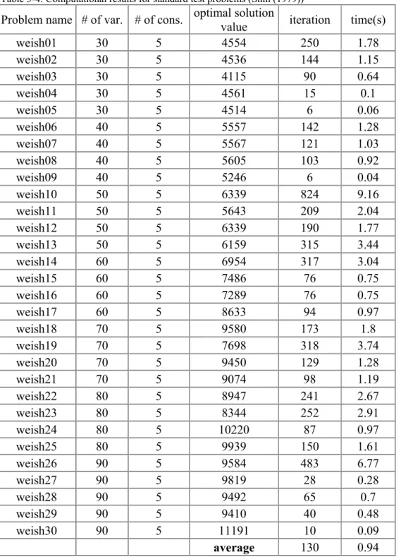
For the first experiment, we have chosen 30 small-sized test problems (Shih (1979)) from the literature which have been used in the computational experimentations of almost all of the algorithms designed for solving the 0-1 MDKP. We were able to solve all of these problems to optimality using the partitioning algorithm, coded in C language. Our computational results regarding these problems are shown in the table below,

Table 3-4: Computational results for standard test problems (Shih (1979))

Problem name # of var. # of cons. optimal solution

value iteration time(s)

weish01 30 5 4554 250 1.78 weish02 30 5 4536 144 1.15 weish03 30 5 4115 90 0.64 weish04 30 5 4561 15 0.1 weish05 30 5 4514 6 0.06 weish06 40 5 5557 142 1.28 weish07 40 5 5567 121 1.03 weish08 40 5 5605 103 0.92 weish09 40 5 5246 6 0.04 weish10 50 5 6339 824 9.16 weish11 50 5 5643 209 2.04 weish12 50 5 6339 190 1.77 weish13 50 5 6159 315 3.44 weish14 60 5 6954 317 3.04 weish15 60 5 7486 76 0.75 weish16 60 5 7289 76 0.75 weish17 60 5 8633 94 0.97 weish18 70 5 9580 173 1.8 weish19 70 5 7698 318 3.74 weish20 70 5 9450 129 1.28 weish21 70 5 9074 98 1.19 weish22 80 5 8947 241 2.67 weish23 80 5 8344 252 2.91 weish24 80 5 10220 87 0.97 weish25 80 5 9939 150 1.61 weish26 90 5 9584 483 6.77 weish27 90 5 9819 28 0.28 weish28 90 5 9492 65 0.7 weish29 90 5 9410 40 0.48 weish30 90 5 11191 10 0.09 average 130 0.94

For the second experiment we randomly generated 0-1 MDKP as follows:

ƒ Each coefficient of the constraint matrix aij (i = 1, . . . , m and j = 1, .

. . , n) and each coefficient of the objective function cj (j = 1, . . . , n)

is an integer randomly chosen between 1 and 1000.

ƒ The right-hand side coefficients (bi ’s) are generated using

n

bi = 0.5

∑

j=1

We made experiments for different values of m and n and found out that if we set m at 5, the largest value of n was 90 for which the algorithm could solve problems to optimality, this value was 40 if we set m at 10 and 25 if we set m at 20. The reason for this is that we limited our algorithm to partitioning the original problem at most 10 times, that is if the first sub-problem is P(T0), then the algorithm stops when it reaches P(T10) (see

section 3.2), due to computational and programming difficulties and to solve larger problems requires using the partitioning procedure more than 10 times.

Note that, the largest values of m and n for which the algorithm solves problems to optimality will be different if one generates easier or harder problems than the ones we generated using the procedure described above. Since the easiest large-sized test problems in the literature are harder than the problems we generated, we conclude that with its current design the partitioning algorithm is not an efficient algorithm to solve large-sized 0-1 MDKP. Therefore, we tried to modify it in such a way that it does not require to use the partitioning procedure a large number of times to solve a

problem. For this purpose, we chose to take advantage of the IP solver of CPLEX to solve sub-problems. Our computational experiments with larger problems showed us that this may be an efficient way to solve large-sized 0-1 MDKP. As it can be seen in the Chapter 5, by this way we are able to find better quality solutions than CPLEX to 0-1 MDKP with large number of variables and few constraints.

The description of the modified partitioning algorithm is given in the next section.

3.5 One Step Partitioning Algorithm

Consider the following 0-1 integer programming problem:

n maximize

∑

∑

1. solve the LP relaxation of the above problem plus any cuts generated so far. Let X* = (x1*, x2*, . . . ,xn*) denote the solution to the LP relaxation.

Stop, if either the problem is infeasible or the objective function value for X* is less than the best feasible integer solution value found so far (Zinc) plus one, declaring Zinc as optimal.

2. generate Xint = (x1', x2', . . . ,xn') as candidate solution by the following:

Check if this solution is feasible and update the incumbent solution if it is feasible and the objective function value associated with it is greater than Zinc.

3. calculate the value of the integrality gap associated with the solution to the LP relaxation as follows:

n

δ = n -

∑

j=1

3.a. If the value of the integrality gap (δ) is less than 1, add the following cut to the problem:

∑

∑

jЄS1 jЄS2

where S1 = { j | xj' = 1} and S2 = { j | xj' = 0}.

Go to 1.

3.b. If the value of the integrality gap (δ) is greater than 1, 3.b.1. partition the problem with T defined as:

T C N = {1, 2, . . . ,n}, and j Є T if max [xj*, (1 - xj*)] = 1, j = 1, . . .,n,

and solve the associated problem P(T): maximize

∑

jЄN\T

subject to

∑

∑

jЄN\T jЄT

xj Є {0, 1}, j Є N \ T

3.b.2. check the candidate solution for feasibility and if it is feasible and the objective function value associated with it is greater than Zinc,

update the incumbent solution.

3.b.3. append a new cut to the original problem as,

∑

∑

jЄT∩S1 jЄT∩S2

where S1 = { j | xj' = 1} and S2 = { j | xj' = 0}.

Go to 1.

As the number of iterations increases, the computational time increases rapidly at each iteration because the number of constraints increases and the problems get larger. Since we use the IP solver of CPLEX to solve sub-problems, the computational time of the algorithm rapidly increases as the sub-problems get larger.

C h a p t e r 4

Computational Analysis of the Search Based

Cuts

4.1 Computational Analysis of the Search Based Cuts Applied

to the 0-1 MDKP

We used the multidimensional 0-1 knapsack problems generated by Chu and Beasley (1998) for the computational analysis of the search based cuts. We made two experiments. In the first experiment, we fixed the number of constraints and for different numbers of variables we calculated the absolute reduction in the objective value per cut after 100 cuts (generated by the one step partitioning algorithm) are added to the original problem. We used 10 problems for each combination of m and n, while m is the number of constraints and n is the number of variables. The results for the first experiment are as follows:

Table 4-1a: Computational results for m=5, α=0.5 and n=100 OR-library instances (see [6]) pb z(1) z(2) |z(1)-z(2)|/ 100 Mkpcb1-11 42939.52 42830.36 1.0916 Mkpcb1-12 42706.7 42613.85 0.9285 Mkpcb1-13 42165.19 42095.35 0.6984 Mkpcb1-14 45347.07 45234.88 1.1219 Mkpcb1-15 42434.12 42328.64 1.0548 Mkpcb1-16 43082.23 42988.35 0.9388 Mkpcb1-17 42190.6 42069.72 1.2088 Mkpcb1-18 45265.47 45171.75 0.9372 Mkpcb1-19 43567.49 43507.01 0.6048 Mkpcb1-20 44796.63 44680.97 1.1566 average 0.97414

Table 4-1b: Computational results for m=5, α=0.5 and n=250 OR-library instances (see [6])

pb z(1) z(2) |z(1)-z(2)|/ 100 mkpcb2-11 109220.6 109186.6 0.340 mkpcb2-12 109960.3 109917.4 0.429 mkpcb2-13 108648.8 108607.1 0.417 mkpcb2-14 109510.8 109472.7 0.381 mkpcb2-15 110834.2 110805.7 0.285 mkpcb2-16 110366.8 110336.1 0.307 mkpcb2-17 109152.6 109126 0.266 mkpcb2-18 109137.7 109113.1 0.246 mkpcb2-19 110123.1 110075.3 0.478 mkpcb2-20 107162.1 107136 0.261 average 0.341

Table 4-1c: Computational results for m=5, α=0.5 and n=500 OR-library instances (see [6]) pb z(1) z(2) |z(1)-z(2)|/ 100 mkpcb3-11 218500.1 218483.1 0.170 mkpcb3-12 221272.4 221253.3 0.191 mkpcb3-13 217615.8 217600.9 0.149 mkpcb3-14 223653.2 223634.9 0.183 mkpcb3-15 219067.5 219042.9 0.246 mkpcb3-16 220617 220602.2 0.148 mkpcb3-17 220076.5 220054.4 0.221 mkpcb3-18 218282.7 218266.5 0.162 mkpcb3-19 217059.9 217043.3 0.166 mkpcb3-20 219812.8 219793.6 0.192 average 0.1828

The first column of the tables above shows the problem name, in the second column the objective value for the LP relaxation of the original problem (z(1)) is given for each problem, z(2) is the objective value for the LP relaxation of the original problem plus 100 cuts generated by the one step partitioning algorithm and finally |z(1)- z(2)| /100 (absolute change in the objective value per cut) is given in column 4.

As seen from the tables above we fixed m at 5 and made computational experiments for n = 100, 250, 500. The average value of the absolute reduction in the objective value per cut after 100 cuts are added is 0.97414 for n = 100, 0.341 for n = 250 and 0.1828 for n = 500. These results are shown in the table and depicted in the graph below,

Table 4-1d: Average value of absolute reduction in objective value per cut for m=5, α=0.5 n |z(1)- z(2)| / 100 100 0.97414 250 0.341 500 0.1828

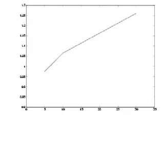
Figure 4-1a: Absolute reduction in the objective value per cut as n increases

As it can be seen from the table, the absolute reduction in the objective value per cut after 100 cuts are added decreases as the number of variables increases. That is, the effectiveness of the search based cuts decrease as the number of variables increases.

In the second experiment, we fixed the number of variables and for different numbers of constraints we calculated the absolute reduction in the objective value per cut after 100 cuts (generated by the one step partitioning algorithm) are added to the original problem. We used 10 problems for each

combination of m and n, while m is the number of constraints and n is the number of variables. The results for the second experiment are as follows:

Table 4-1e: Computational results for n=100, α=0.5 and m=5 OR-library instances (see [6])

pb z(1) z(2) |z(1)-z(2)| / 100 mkpcb1-11 42939.52 42830.36 1.0916 mkpcb1-12 42706.70 42613.85 0.9285 mkpcb1-13 42165.19 42095.35 0.6984 mkpcb1-14 45347.07 45234.88 1.1219 mkpcb1-15 42434.12 42328.64 1.0548 mkpcb1-16 43082.23 42988.35 0.9388 mkpcb1-17 42190.6 42069.72 1.2088 mkpcb1-18 45265.47 45171.75 0.9372 mkpcb1-19 43567.49 43507.01 0.6048 mkpcb1-20 44796.63 44680.97 1.1566 average 0.97414

Table 4-1f: Computational results for n=100, α=0.5 and m=10 OR-library instances (see [6])

pb z(1) z(2) |z(1)-z(2)|/ 100 mkpcb4-11 41712.64 41622.68 0.8996 mkpcb4-12 42597.32 42504.68 0.9264 mkpcb4-13 42759.32 42643.13 1.1619 mkpcb4-14 45959.36 45862.18 0.9718 mkpcb4-15 42183.12 42076.02 1.0710 mkpcb4-16 43377.96 43265.22 1.1274 mkpcb4-17 43927.94 43820.5 1.0744 mkpcb4-18 43335.83 43220.3 1.1553 mkpcb4-19 42611.6 42494.93 1.1667 mkpcb4-20 41542.79 41433.04 1.0975 average 1.0652

Table 4-1g: Computational results for n=100,α=0.5 and m=30 OR-library instances (see [6]) pb z(1) z(2) |z(1)-z(2)| / 100 mkpcb7-11 41276.36 41173.16 1.0320 mkpcb7-12 41866.73 41740.82 1.2591 mkpcb7-13 42232.96 42124.72 1.0824 mkpcb7-14 41634.88 41510.52 1.2436 mkpcb7-15 41410.88 41323.66 0.8722 mkpcb7-16 41603.16 41468.19 1.3497 mkpcb7-17 41616.13 41500.70 1.1543 mkpcb7-18 43388.05 43207.30 1.8075 mkpcb7-19 42656.56 42533.10 1.2346 mkpcb7-20 42262.70 42105.70 1.5700 average 1.26054

As seen from the tables above we fixed n at 100 and made computational experiments for m = 5, 10, 30. The average value of the absolute reduction in the objective value per cut after 100 cuts are added is 0.97414 for m = 5, 1.0652 for m = 10 and 1.26054 for m = 30. These results are shown in the table and depicted in the graph below,

Table 4-1h: Average value of absolute reduction in objective value per cut for n=100, α=0.5

m |z(1)-z(2)|/ 100

5 0.97414

10 1.0652 30 1.26054

Figure 4-1b: Absolute reduction in the objective value per cut as m increases

As it can be seen from the table, the absolute reduction in the objective value per cut after 100 cuts are added increases as the number of constraints increases. That is, the effectiveness of the search based cuts increase as the number of constraints increases.

4.2 Computational Analysis of the Search Based Cuts Applied

to the Set Covering Problem

For the second part of the computational analysis of the search based cuts we used another well known combinatorial optimization problem which is the set covering problem. The set covering problem can be formulated as follows: n minimize

∑

∑

where aij Є {0, 1} for i = 1, . . . , m; j = 1, . . . , n; and cj > 0 for j = 1, . . .,n.

For our computational experiments, we randomly generated set covering problems by the following:

ƒ Each coefficient of the constraint matrix aij (i = 1, . . . , m and j = 1, . .

. ,n) is 1 with probability 0.5 and 0 with probability 0.5 . ƒ Each coefficient of the objective function cj (j = 1, . . . , n) is 1.

In order to analyze the effectiveness of the search based cuts, we made two experiments. In the first experiment, we fixed the number of constraints and for different numbers of variables we calculated the absolute increase in the objective value per cut after 100 cuts (generated by the one step partitioning algorithm) are added to the original problem. We used 5 problems for each

combination of m and n, and the results for the first experiment are as follows:

Table 4-2a: Computational results for m=5 and n=100 set covering problems

pb z(1) z(2) |z(1)-z(2)| / 100 sc1 1.25 1.661876 0.004119 sc2 1.25 1.705390 0.004554 sc3 1.25 1.735886 0.004859 sc4 1.25 1.710705 0.004607 sc5 1.25 1.771835 0.005218 average 0.004671

Table 4-2b: Computational results for m=5 and n=150 set covering problems

Pb z(1) z(2) |z(1)-z(2)| / 100 Sc6 1.25 1.580607 0.003306 Sc7 1.25 1.598384 0.003484 Sc8 1.25 1.597140 0.003471 Sc9 1.333333 1.538552 0.002052 Sc10 1.25 1.597115 0.003471 average 0.003157

Table 4-2c: Computational results for m=5 and n=200 set covering problems

Pb z(1) z(2) |z(1)-z(2)| / 100 Sc11 1.25 1.532358 0.002824 sc12 1.25 1.518742 0.002687 sc13 1.25 1.498249 0.002482 sc14 1.25 1.504127 0.002541 sc15 1.25 1.537601 0.002876 average 0.002682

The first column of the tables above shows the problem name, in the second column the objective value for the LP relaxation of the original problem (z(1)) is given for each problem, z(2) is the objective value for the LP relaxation of the original problem plus 100 cuts generated by the one step partitioning algorithm and finally |z(1)- z(2)| /100 (absolute change in the objective value per cut) is given in column 4.

As seen from the tables above we fixed m at 5 and made computational experiments for n = 100, 150, 200. The average value of the absolute increase in the objective value per cut after 100 cuts are added is 0.004671 for n = 100, 0.003157 for n = 150 and 0.002682 for n = 200. These results are shown in the table and depicted in the graph below,

Table 4-2d: Average value of absolute increase in the objective value per cut for m=5

n |z(1)- z(2)| / 100

100 0.004671

150 0.003157 200 0.002682

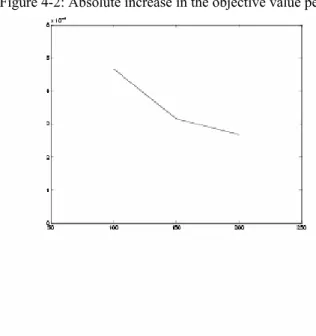
Figure 4-2: Absolute increase in the objective value per cut as n increases

As it can be seen from the table, the absolute increase in the objective value per cut after 100 cuts are added decreases as the number of variables increases. That is, the effectiveness of the search based cuts decreases as the number of variables increases as in the case of the 0-1 MDKP.

In the second experiment, we fixed the number of variables and for different numbers of constraints we calculated the absolute increase in the objective value per cut after 100 cuts (generated by the one step partitioning algorithm) are added to the original problem. We used 5 problems for each combination of m and n, and below are the results for the second experiment:

Table 4-2e: Computational results for n=100 and m=5 set covering problems pb z(1) z(2) |z(1)-z(2)| / 100 sc1 1.25 1.661876 0.004119 sc2 1.25 1.705390 0.004554 sc3 1.25 1.735886 0.004859 sc4 1.25 1.710705 0.004607 sc5 1.25 1.771835 0.005218 Average 0.004671

Table 4-2f: Computational results for n=100 and m=10 set covering problems

pb z(1) z(2) |z(1)-z(2)| /100 sc16 1.2 1.883667 0.006837 sc17 1.333333 1.889595 0.005563 sc18 1.25 1.764056 0.005141 sc19 1.2 1.821188 0.006212 sc20 1.285714 1.857548 0.005718 Average 0.00589

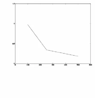
As seen from the tables above, we fixed n at 100 and made computational experiments for m = 5, 10. The average value of the absolute increase in the objective value per cut after 100 cuts are added is 0.004671 for m = 5, and 0.00589 for m = 10. These results are shown in the table below,

Table 4-2g: Average value of absolute increase in the objective value per cut for n=100

m |z(1)-z(2)|/ 100

5 0.004671

As it can be seen from the table, the absolute increase in the objective value per cut after 100 cuts are added increases as the number of constraints increases. That is, the effectiveness of the search based cuts increases as the number of constraints increases as in the case of the 0-1 MDKP.

C h a p t e r 5

Application of the Partitioning Algorithm to the

Multidimensional 0-1 Knapsack Problem

In order to check the efficiency of the partitioning algorithm, the one step partitioning algorithm described in Section 3.5 and coded in C language was applied to 60 randomly generated 0-1 MDKP and 30 large-sized 0-1 MDKP from the literature (Chu and Beasley (1998)). The computational results were compared with the implementation of CPLEX v8.1 in MIP mode and the results reported by Chu and Beasley (1998).

5.1 Problem generation

We generated a set of large 0-1 MDKP instances using the procedure suggested by Freville and Plateau (1994) and used by Chu and Beasley (1998) to generate the standard test problems in OR-library. The number of constraints m was set to 10 and the number of variables n was set to 1000 and 2000. We generated 30 problems for each m-n combination, giving a total of 60 problems.

Each problem instance is randomly generated as follows:

ƒ Each coefficient of the constraint matrix aij (i = 1, . . . , m and j = 1, .

ƒ The right-hand side coefficients (bi ’s) are found using

n

bi = α

∑

j=1

ten problems, α = 0.50 for the next ten problems and α = 0.75 for the remaining ten problems.

ƒ The objective function coefficients (cj ’s) are correlated to aij and

generated by: n

cj =

∑

j=1

where qj is an integer randomly chosen between 1 and 1000. In

general, correlated problems are more difficult to solve than uncorrelated problems (Gavish and Pirkul (1985), Pirkul (1987)).

5.2 Computational Results

The results obtained are shown on Tables 5-2a, 5-2b and 5-2c where, for each problem instance, the following information is given:

ƒ n and m: number of variables and number of constraints. ƒ α: tightness ratio.

ƒ z(lp): optimal value of the LP relaxation of 0-1 MDKP.

ƒ initial value (partitioning algorithm): first feasible integer solution value found by one step partitioning algorithm.

ƒ best value (partitioning algorithm): best feasible integer solution value found by one step partitioning algorithm in 225 iterations.

ƒ iter.: the number of iterations required by one step partitioning algorithm to find the value in column 5.

ƒ time (partitioning algorithm): computation time (in CPU seconds) required by one step partitioning algorithm to find the value in column 5.

ƒ initial value (CPLEX): first feasible integer solution value found by CPLEX v8.1 in MIP mode.

ƒ best value (CPLEX): best feasible integer solution value found by CPLEX v8.1 in MIP mode before memory tree size of 250 Mb is exceeded.

ƒ time (CPLEX): computation time (in CPU seconds) required by CPLEX v8.1 in MIP mode until 250 Mb tree memory size is exceeded.

Table 5-2a: Computational results for n=500 and m=10 OR-library instances (see [6])

Partition Algorithm CPLEX Prob. name z(lp)

initial best iter. time initial best time mkpcb6-01 118019.5 117168 117779 72 9.6 116510 117712 603.98 mkpcb6-02 119437.3 118613 119165 172 135.2 118543 119158 650.96 mkpcb6-03 119405.7 118761 119194 210 443.87 118705 119211 532.23 mkpcb6-04 119066.1 118268 118813 156 82.35 118163 118813 631.62 mkpcb6-05 116698 115896 116509 188 171.01 115379 116423 557.77 mkpcb6-06 119710 118946 119463 188 197.7 118355 119448 577.63 mkpcb6-07 120033.3 119180 119777 168 114.77 118688 119777 576.10 mkpcb6-08 118545.7 117883 118323 128 63.12 117561 118266 611.74 mkpcb6-09 118001.6 117182 117776 170 85.31 116727 117779 561.42 mkpcb6-10 119440.6 118943 119163 160 80.45 118040 119191 613.79 mkpcb6-11 217552.9 217068 217341 190 336.27 216744 217312 633.38 mkpcb6-12 219255.2 218307 219030 164 255.73 218742 219027 536.46 mkpcb6-13 217987.8 217500 217792 146 57.75 216788 217792 537.22 mkpcb6-14 217040.7 216455 216851 154 75.83 215956 216851 678.05 mkpcb6-15 214010.3 212415 213830 200 229.71 213229 213827 590.07 mkpcb6-16 215261.3 214654 215041 224 260.1 214349 215034 582.36 mkpcb6-17 218109.2 217030 217899 194 307.45 217249 217875 622.92 mkpcb6-18 220175.6 219488 219984 102 27.49 218784 219965 606.38 mkpcb6-19 214561 213918 214329 212 449.42 213666 214312 508.71 mkpcb6-20 221083.6 220367 220852 204 186.4 219930 220846 596.21 mkpcb6-21 304555 304214 304334 156 70.76 303606 304344 582.11 mkpcb6-22 302553 301951 302333 176 49.2 302159 302326 461.06 mkpcb6-23 302581.5 300585 302416 82 12.65 302061 302386 581.82 mkpcb6-24 300956.7 300440 300747 128 56.9 300353 300719 455.72 mkpcb6-25 304584.7 303763 304349 196 371.82 303563 304346 548.79 mkpcb6-26 301952.5 301489 301767 148 81.18 301226 301742 537.43 mkpcb6-27 305139.7 304745 304949 128 29.1 304641 304949 538.1 mkpcb6-28 296636.6 296287 296441 158 50.21 296038 296441 551.31 mkpcb6-29 301547.6 301131 301326 164 211.01 300507 301353 606.75 mkpcb6-30 307250 306393 307072 218 138.5 306730 307038 564.21 average 165 154.7 average 574.54