Investigating Use of Pressure Pulses to Assess Near Wellbore Reservoir Parameters

INVESTIGATING USE OF PRESSURE PULSES TO ASSESS NEAR WELLBORE RESERVOIR PARAMETERS

1_{İsmail DURGUT,} 2_{Jon S. GUDMUNDSSON,} 3_{Alberto Di LULLO}

1_{Department of Petroleum Natural Gas Engineering, Middle East Technical University, Ankara, Turkey} 2_{(Retired) Department of Petroleum Engineering and Applied Geophysics, NTNU, Trondheim, Norway} 3_{Flow Assurance Engineering Technologies, ENI, Upstream and Technical Services, San Donato Milanese,}

Italy

1_{durgut@metu.edu.tr,} 3_{alberto.dilullo@eni.com}

Geliş/Received: 16.10.2018; Kabul/Accepted in Revised Form: 26.02.2019)

ABSTRACT: Pressure surge in a pipe due to sudden flow rate change or full-stop of fluid flow is a

pressure wave propagating in fluid along the pipe. This phenomenon has been used to determine the flow rate and to detect and monitor changes in effective flow diameter. It turns out that the pressure surge, also known as pressure pulse, can be used to estimate the formation transmissivity and storativity in the near wellbore region. In this study, propagation of pressure pulse generated by sudden valve closure is simulated with a transient pipe flow model, and it is coupled with a transient analytical reservoir model. The coupled model is used to estimate the reservoir parameters by history matching approach, which is to iterate the transmissivity and the storativity values until an acceptable match is obtained between the measured and simulated pressure history at the upstream of valve. The developed modeling and estimation scheme is applied with two data sets from a field well test to estimate reservoir parameters. The reservoir parameters transmissivity and storativity in the near wellbore region were obtained from the history matching analysis. Matching analysis with the coupled model on the recorded wellhead pressure during two tests showing obvious different flowing conditions points out very similar reservoir parameter values.

Key Words: Pressure waves, Reservoir parameters, Transient pipe flow, Water hammer

Kuyu Yakınında Rezervuar Parametrelerinin Belirlenmesinde Basınç Darbesinin Kullanılmasının İncelenmesi

ÖZ: Bir akışkanın aktığı boruda ani akış hızı değişikliği veya akışın aniden durdurulması boru

içerisinde yayılan basınç dalgalanmasına sebep olur. Bu doğal olgu akış hızının ölçümü ve borunun etkin çapının belirlenmesi ve gözlenmesi hesaplamalarında kullanılmıştır. Basınç darbesi olarak da bilinen basınç dalgası kuyu yakınında formasyon geçirimliliği ve storativitesinin tahmininde kullanılabileceği öngörülmektedir. Bu çalışmada, ani vana kapanmasıyla oluşturulan basınç darbesinin yayılımı geçici rejim boru akış modeli ile simüle edilip, bu model analitik geçici rejim rezervuar modeli ile birleştirilmiştir. Birleştirilen model, vana girişinde ölçülen ve hesaplanan basınç değişim verilerini eşleştirme yaklaşımıyla rezervuar parametrelerinin iteratif olarak tahmini işleminde kullanılmıştır. Geliştirilen bu modelleme ve tahmin yaklaşımı bir kuyudaki iki kuyu test verisine rezervuar parametrelerini tahmin etme amacıyla uygulanmıştır. Kuyu civarındaki geçirimlilik ve storativite değerleri ölçülen/hesaplanan veri eşleştirme yöntemiyle elde edilmiştir. Kuyuda iki farklı akış durumunda ölçülen basınç değişimi bilgisinin birleştirilmiş modelle gerçekleştirilen eşleştirme analizi rezervuar parametreleri için çok benzer değerleri işaret etmektedir.

INTRODUCTION

Sudden rate change or full-stop of fluid flow in a conduit causes a pressure surge called water hammer, also known as a pressure pulse. When a valve is activated quickly, the pressure pulse (i.e. compression or expansion type pressure wave) generated propagates upstream and downstream. This phenomenon has been known for centuries (Mambretti, 2005) however, a Russian professor Nikolay Joukowsky was the first to describe the phenomenon theoretically and to define “the fundamental equation of water hammer” which is the best-known equation in transient flow theory. Therefore, this equation is known as Joukowsky equation (Ghidaoui et al., 2005). Moreover, his experimental work showed also that the water hammer waves propagate in piping system with a constant speed, which is independent of the shock intensity but depend on the pipe material and the pipe wall thickness (Prümmer, 2009).

The petroleum industry recognizes the potential effect and use of the phenomenon, however mostly from operational perspective. For instance, Santarelli et al. (2000)investigated the effect of water hammer on triggering sand liquefaction and production in water injectors; Zazovsky et al.’s (2014) evaluated the impact of pressure pulse generated by valve closure on formation, which might cause damage and transient sand production. Some other work has also been done on downhole formation damage and sand stability subject to water hammer waves (Vaziri et al., 2007; Wang et al., 2008). Livescu and Watkins (2014) investigated the water hammer pulses on the radial vibrations in coiled tubings and developed a model to simulate vibrations of the coil tubings with water hammer pulses.

Besides, pressure pulses can also be used to meter flows and to detect and monitor deposits. Gudmundsson and Celius (1999) showed the applicability of pressure pulse method for allocation testing and wellbore monitoring. Gudmundsson et al. (2001) applied pressure pulse to detect deposits in pipelines. Recently Carey et al. (2015) suggested that hydraulic fracture parameters could be estimated from the water hammer pressure signature by using a transient pipe flow model.

In this study we propose that the storativity and transmissivity of a reservoir near the wellbore can be estimated by using the pressure signal generated by a quick closing valve. The signal measured at upstream of the valve is analyzed by using coupled transient pipe flow and transient analytical reservoir models. The transient pipe flow model simulates the propagation of pressure wave/pulse generated by sudden valve closure in a pipe. The reservoir model, which is implemented as the boundary condition of the transient pipe flow model simulates the reservoir response to the pressure transients at the sand face. The reservoir parameters near wellbore region will be obtained by the history matching analysis using the coupled models.

MATERIALS AND METHODS

Quick-closing valve generates a pressure pulse, which propagates in the flowing fluid (both upstream and downstream). This pulse stops the flow while traveling in both directions. However, the complete stop takes place at the valve only, because the pulse dampens as the additional pressure required to keep the fluid flowing against the frictional force is released. In the rest of the pipe, the flow velocity will reduce gradually. The reduction of flow velocity is a function of the remained strength of the pulse. In other words, the ever decreasing kinetic energy of the pulse can only decelerate the fluid flow (i.e. cannot completely put the fluid at rest).

When the pulse reaches the bottom hole, it also changes the flow from (or into) the reservoir. As the pulse reflects back from the bottom hole, it also generates pressure transients in the reservoir. Then it propagates toward the wellhead, where it reflects back again. As stated earlier, the pulse strength (i.e. the amplitude of the water hammer pressure wave) is weakened by the frictional losses as the pulse propagates. If the pressure pulse is strong enough, the reflections may repeat tens of times until the pressure pulse attenuates completely. Therefore, a transient pipe flow model coupled with a reservoir flow models required to simulate both the propagation of pressure pulse and the pressure transients in the reservoir.

Modelling Transient Fluid Flow in Pipe

The transient flow model solves the equations describing the transient flow of single-phase viscous fluid in a pipe. These equations are mass and momentum balance equations for unsteady pipe flow in one dimension; given below respectively (Chevray and Mathieu, 1993):

𝜕(𝐴𝜌) 𝜕𝑡 + 𝜕(𝐴𝜌𝑣) 𝜕𝑥 = 0 ( 1) 𝜕(𝐴𝜌𝑣) 𝜕𝑡 + 𝜕(𝐴𝜌𝑣|𝑣|) 𝜕𝑥 + 𝜕(𝐴𝑝) 𝜕𝑥 = − 𝑓 2𝐷𝜌𝑣|𝑣|𝐴 + 4 3 𝜕 𝜕𝑥(𝐴𝜇 𝜕𝑣 𝜕𝑥) − 𝐴𝜌𝑔 𝑑𝑧 𝑑𝑥 ( 2) where 𝑣 = 𝑣(𝑥, 𝑡)is the cross-sectional average fluid flow velocity in the direction𝑥(along the pipe) and at the time 𝑡, 𝑝 = 𝑝(𝑥, 𝑡) the pressure, 𝜌 = 𝜌(𝑥) the fluid density, 𝜇 = 𝜇(𝑥) the dynamic viscosity of fluid, 𝐷 = 𝐷(𝑥) the flow diameter, 𝐴 = 𝐴(𝑥) the flow area, 𝑔 the acceleration of gravity, and 𝑧 is the opposite direction of gravity.

Although the energy balance equation is excluded from the system of equations, it does not imply the assumption of isothermal flow condition, because the density and viscosity are considered to vary with distance, which may reflect non-isothermal flow condition along the pipe.

The pressure transients (the pressure waves generated by the valve action) in fluid-filled pipe propagate with the in-situ speed of sound, which can be defined as (Howe 2006):

𝑐 = (𝜕𝑝 𝜕𝜌)

0.5

(3) Using the definition of the speed of sound, introducing the mass rate as 𝑚 = 𝜌𝑣𝐴,and neglecting the viscous term; one can transform Eqs. 1 and 2 to

𝜕𝑝 𝜕𝑡+ 𝑐2 𝐴 𝜕𝑚 𝜕𝑥 = 0 (4) 𝜕𝑚 𝜕𝑡 + (1 − ( 𝑣 𝑐) 2 ) 𝐴𝜕𝑝 𝜕𝑥+ 2𝑣 𝜕𝑚 𝜕𝑥 = − 𝑓 2𝐷 𝑚|𝑚| 𝜌𝐴 − 𝐴𝜌𝑔 𝑑𝑧 𝑑𝑥 (5)

The set of partial differential equations describing propagation of Pressure Pulse is solved by a numerical solver, called Clawpack (Conservation LAWs PACKage), which is a collection of algorithms applying finite volume methods for solving time-dependent hyperbolic equations. Information about the details of solution methodology can be found somewhere else (LeVeque 2002, Falk 1999).

Initialization of Transient Fluid Flow Model

The solution method needs to set state variables at the time 𝑡 = 0. The initialization assumes no variation in the pressure and the mass rate with time before closure (i.e. the steady-state flow condition).Therefore, the pressure along the pipe is simply obtained by the steady state solution of the governing equations (Eqs. 4 and 5), which yields

𝜕𝑝 𝜕𝑥= − [ 𝑓 2𝐷 𝑚|𝑚| 𝜌𝐴 − 𝐴𝜌𝑔 𝑑𝑧 𝑑𝑥] [(1 − ( 𝑣 𝑐) 2 ) 𝐴] ⁄ (6)

This equation is solved numerically for each cell starting from the pipe end with valve where the pressure and the rate is known before the valve closure. The discretized form of Eq.6 initializes the cell values, which are evaluated at the center of the cell:

𝑝_𝑖+1= 𝑝_𝑖− [ 𝑓𝑖 2𝐷_𝑖 𝑚0_|𝑚0_| 𝜌_𝑖𝐴_𝑖 − 𝐴𝑖𝜌𝑖𝑔 𝑑𝑧 𝑑𝑥] [(1 − ( 𝑣𝑖 𝑐_𝑖) 2 ) 𝐴_𝑖] ⁄ ∆𝑥 (7)

where 𝑚0 is the initial mass flow rate and 𝑝0 is the pressure at the valve. It has a negative value if the direction of flow is from the pipe towards the valve (and then out of the valve), and it is positive for the reverse direction.

Boundary Conditions of Transient Fluid Flow Model

In addition to initial conditions, the solution to a hyperbolic problem in a limited spatial domain, the numerical algorithm requires boundary conditions to have well-posed problem. Since the system is disturbed by an event, which is indeed the valve closure, it causes a wave propagating down the well.

At the well head, the flow rate changes during the valve closure event, which is modeled as reduction of mass rate in a given period. This is achieved by setting the mass rate at the valve-grid to decreasing values (starting from initial value to zero) during closing period. After the valve is fully closed, the valve is described by a closed-end boundary.

For the other end, i.e. the bottom hole, the constant pressure or constant rate condition can be applied. If the bottom hole boundary condition is set to a constant value, during the simulation run it is kept at its initial steady state value. However, the pressure pulse causing pressure transients in the wellbore causes also pressure transient in the reservoir around the wellbore. Therefore, an infinite acting reservoir model is implemented into the transient fluid flow model. The reservoir model is detailed in Section 2.4.

Reservoir Model

The model of reservoir is a horizontal radial flow model in a homogeneous porous medium saturated with a slightly compressible fluid. It is also assumed that the reservoir has uniform thickness and isotropic permeability and has been perforated over the entire reservoir thickness. Under these assumptions, one can derive an equation, which describes the pressure at any time at any point in the porous medium: the well-known general diffusivity equation. It can be solved analytically under pre-defined conditions.

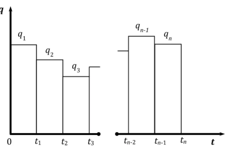
One of the analytical solutions is the line source solution, which presupposes radial flow in an infinite acting reservoir with a wellbore of zero radius. The line source solution also assumes constant well flow rate at the sandface (Chierici 1994). However, the pressure pulse itself is a rapid transient in pressure, and therefore its effect on the flow from and/or to the reservoir is transient too. Therefore, the reservoir has to be put on flowing at a discrete flow rate history, which has stepwise variation with time (see Figure 1). The flow history is as follows:

Flow rate Duration 𝑞₁ 𝑡₁− 0 𝑞2 𝑡2− 𝑡1 𝑞₃ 𝑡₃− 𝑡₂

… …

Figure 1. Time-varying flow rate for use with the principle of superposition in time

Applying the principle of superposition in time to the general solution of diffusivity equation, one can obtain the bottom hole pressure response from:

𝑝_𝑤𝑓(𝑡_𝑛) = 𝑝_𝑖− 1

2𝜇𝑇{∑(𝑞𝑗− 𝑞𝑗−1) [𝑝𝐷(𝑡𝐷(𝑡𝑗) − 𝑡𝐷(𝑡𝑗−1))] 𝑛

𝑗=1

} (8)

where 𝑝𝐷(∙)is the dimensionless form of the line source solution given as 𝑝_𝐷(𝑡_𝐷) =1

2𝐸𝑖( 1

4𝑡_𝐷) (9)

by introducing the dimensionless time and the supplementary definitions for the reservoir rock and fluid parameters: Transmissivity: 𝑇 =𝑘ℎ 𝜇 (10.a) Storativity: 𝑆 = 𝜙𝑐𝑡ℎ (10.b) Dimensionless time: 𝑡_𝐷= 𝑘 𝜙𝜇𝑐_𝑡𝑟_𝑤2𝑡 = 𝑇 𝑆𝑟_𝑤2𝑡 (10.c)

with consistent units i.e. 𝑘 in m2_{, ℎ in m, 𝜇 Pa·s, 𝑇 in m}3_{/Pa·s, 𝑐}

𝑡 in 1/Pa, 𝑆 in m/Pa, 𝜙 in fraction, 𝑟𝑤 in m and 𝑡 in s.

The pipe-flow model calculates pressure and mass rate inside the pipe by using a known pressure boundary condition, which is indeed the bottom hole sandface pressure calculated by the reservoir model. The reservoir model takes the flow rate from the pipe model and calculates the sandface pressure, which is to be used as the boundary condition in the pipe-flow model at the next time step. This step needs to get 𝑝𝑤𝑓 from Eq.8 by the known flow rate history (i.e. the flow rates in every time steps).

Since the well is flowing before the pressure pulse test, the reservoir model needs to be put on flow at a known constant rate q for a given initialization period in order to generate pressure profile in the reservoir. The superposition calculations always start with this prolonged initial flow period over the initial reservoir pressure, which is taken as the pressure at the radius of investigation. The pressure response follows a diffusion type response, which implies that a pressure change at the well would be felt at least infinitesimally everywhere in the reservoir. However, from a practical standpoint there will be some point distant from the well at which the pressure response is so small as to be undetectable. The distance is indeed the radius of investigation. Since its definition depends on arbitrary variation in pressure response, there has been a variety of definitions in the literature. One way is in terms of the time at which the effect of boundaries in a closed reservoir is seen (Horne 1995). This way needs to re-define the dimensionless time based upon reservoir area:

𝑡𝐷𝐴 = 𝑘𝑡 𝜙𝜇𝑐𝑡𝐴𝑟𝑒𝑠 or 𝑡𝐷𝐴 = 𝑇 𝑆𝜋𝑟𝑒2𝑡 (11) q₁ q₂ q₃ q_n-1 q_n q t 0 t1 t2 t3 tn-2 tn-1 tn

If no boundary effect has been seen at a particular time during a test, then the dimensionless time 𝑡𝐷𝐴 for the radius of investigation at that moment must be less than 0.1. This basis gives rise to the following expression for radius of investigation:

𝑟_𝑖𝑛𝑣 = ( 𝑇 0.1𝜋𝑆𝑡)

0.5

(12) Long enough initialization time (which is a parameter of the reservoir model) guarantees that the pressure transients caused by the pressure pulse cannot reach practically beyond the radius of investigation. Hence, the pressure at this distance does not change practically; it can be used as the initial reservoir pressure for initialization purpose.

RESULTS AND DISCUSSION

The proposed approach and the developed model is applied, first, on an illustrative case to demonstrate the effect of reservoir parameters on the model response. Afterwards, we performed simulations with two data sets from field tests to estimate reservoir parameters.

Illustrative Simulation Case Study: Effect of Reservoir Parameters

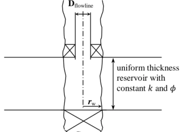
The first series of simulations presented in this paper are carried out to demonstrate the effect of reservoir parameters. A well is producing from a uniform thickness homogenous reservoir at 4000 m depth with constant rate. The well is installed with 3½ in. production tubing (ID 74.2 mm). It is completed as open-hole with the wellbore diameter of 10 cm (see Figure 2). The formation thickness is 50 m. While the well is flowing at a constant rate of 3 kg/s the valve in the wellhead is closed in one second. It is assumed that the fluid parameters remain constant with time and distance; the density is 700 kg/m3 and the sound velocity is 1000 m/s.

Figure 2. Reservoir and well completion for a test simulation

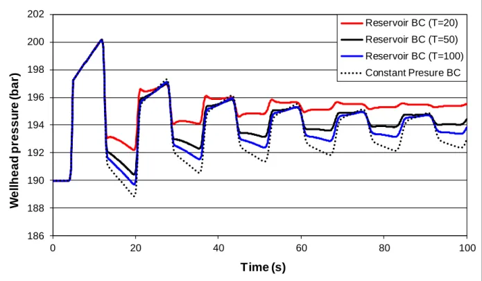
The effect of transmissivity and storativity is investigated with two sets of simulations. The first one is to show the effect of transmissivity while the second one is for the storativity. In each set of simulations, when one parameter is changed the other parameter is kept constant. Simulation results are presented in Figures 3 and 4. These figures compare the simulated wellhead pressures by the different transmissivities and storativities. As seen in Figure 3, decreasing transmissivity causes stronger attenuation of pulse in addition to increasing the average level of reflecting pulse, in other words increasing the level at which the pulse dies out. Moreover, the storativity behaves likewise, i.e. lower the storativity stronger the attenuation, but this parameter is not effective as transmissivity (compare Figure 3 with Figure 4). The reason is obvious that the transient pressure response is linearly related with the inverse of the transmissivity while it is logarithmic with the storativity, therefore the transmissivity is the dominant factor.

Dflowline

rw

uniform thickness reservoir with constant 𝑘 and 𝜙

Figure3. Wellhead pressures obtained by simulations applying reservoir boundary condition with

transmissivities of 20, 50 and 100 Darcy-m/cp respectively and constant storativity of 10-3 _m/bar

Figure 4. Wellhead pressures obtained by simulations applying reservoir boundary condition with

storativities of 10-4_{, 10}-3 _{and 10}-2 _{m/bar respectively and constant transmissivity of 50 Darcy-m/cp}

The pressure-pulse changes the pressure at the sandface, which gives rise to change in inflow from the reservoir. If the reservoir has less resistance to follow the pressure of pulse, it will react more closely

186 188 190 192 194 196 198 200 202 0 20 40 60 80 100

W

e

ll

h

e

a

d

p

re

s

s

u

re

(

b

a

r)

Time (s)

W

e

ll

h

e

a

d

p

re

s

s

u

re

(

b

a

r)

Time (s)

to a huge constant pressure reservoir and will be ready to give as much fluid flow as the pressure-pulse needs to keep the pressure back to its original value. However, if it resists, there will be pressure equalization at sandface, and then the fast transient in pressure will retain the change at least in an infinitesimal extent in the reservoir for some time, which will result in removing some kinetic energy from the pressure-pulse and will cause consecutively the attenuation of pulse. This phenomenon can be seen more at low permeability, low porosity, tight (less compressible) reservoirs.

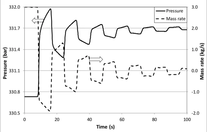
The simulator provides also the pressure and the mass rate at the bottom hole. Figure 5 illustrates how the pressure builds up after the valve closure and how the flow direction changes due to the pressure wave reflecting back and forth in the production tubing. For this case, the reservoir boundary condition with is applied with the storativity of 10-3 _{m/bar and the transmissivity of 50 Darcy-m/cp. The} results show that the sudden valve closure on the surface does not stop the production from reservoir immediately, instead the repeating pressure pulse changes the flow direction and causes swing in the flow direction and the bottom hole pressure which is also reflected on the surface pressure measurement.

Figure 5. Sandface pressure and mass rate obtained by simulation applying reservoir boundary

condition with storativity of 10-3 _{m/bar and transmissivity of 50 Darcy-m/cp}

Moreover, the developed simulator has a feature to calculate the pressure profile in the reservoir at each time step. Figure 6 shows those profiles at different times again for the reservoir boundary condition with the storativity of 10-3 _{m/bar and the transmissivity of 50 Darcy-m/cp. The profiles clarify} what happens inside the reservoir.

The water hammer pressure, which is approximately 7 bars at the wellhead hits the reservoir with a reduced pressure surge (less than one bar, see Figure 5) at around 8th _{second and it increases the} sandface pressure 0.9 bar in 1 second (Figure 6.a). Remember that the valve was closed in 1 second. As the pressure wave penetrates into the reservoir, this causes a reverse pressure gradient along a short distance in the reservoir, which is indication of inflow to the reservoir (i.e. changing flow direction).

-2.0 -1.0 0.0 1.0 2.0 3.0 330.5 330.8 331.1 331.4 331.7 332.0 0 20 40 60 80 100

M

as

s

ra

te

(

kg

/s

)

P

re

ss

u

re

(

b

ar

)

Time (s)

Note that as the pressure pulse reflects back from the sandface, its phase changes as well (i.e. the pressure pulse becomes a wave with decreasing pressure). This negative pulse travels back into the wellbore. When the pulse reached back to the reservoir for the second time (Figure 6.b), it was actually a wave with decreasing pressure, which results in flow from the reservoir into the wellbore. The sequence of first increasing then decreasing pressure waves repeats until the pressure pulse disappears.

“

Figure 6. Reservoir pressure profiles at different times obtained by simulation applying reservoir

boundary condition with storativity of 10-3 _{m/bar and transmissivity of 50 Darcy-m/cp}

The pressure profiles indicate another detail that the pressure surge generated by a valve closure results in oscillating behavior of the reservoir pressure. The pressure disturbances can only penetrate several meters into the reservoir for the duration of pressure pulse tests. Therefore, the pressure response at the wellhead should reflect effect of the reservoir properties near the wellbore.

Field Case Studies

The second set of study is a field case where the pressure pulse method is applied in a single-phase oil production well.

The method has been tested in an oil production well producing from a deep carbonate reservoir. The length of wellbore is 5500 m. A 3½ in. by 2⅞ in. (8.89 mm by 7.30 mm) nominal diameter tapered production tubing string has been run in the well. The smaller diameter tubing is anchored to the surface tubing at 1675 m.

The wellbore had flow assurance solids problem; it has been therefore cleaned up. The pressure pulse tests have been performed before and after the wellbore cleanup operation.

The data set, which is to be discussed first, belongs to the condition after the cleanup operation because the recorded data is longer.

330.6 330.8 331.0 331.2 331.4 331.6 331.8 332.0 0.1 1 10 100 R es er vo ir p er ss u re (b ar ) Distance (m) Initial, < 8.0 s. 8.4 s. 8.7 s. 9.1 s. 16.0 s. (a) 330.6 330.8 331.0 331.2 331.4 331.6 331.8 332.0 0.1 1 10 100 R es er vo ir p er ss u re (b ar ) Distance (m) 16.0 s. 16.6 s. 17.1 s. 24.0 s. (b) 330.6 330.8 331.0 331.2 331.4 331.6 331.8 332.0 0.1 1 10 100 R es er vo ir p er ss u re (b ar ) Distance (m) 24.0 s. 24.7 s. 25.1 s. 32.0 s. (c) 330.6 330.8 331.0 331.2 331.4 331.6 331.8 332.0 0.1 1 10 100 R es er vo ir p er ss u re (b ar ) Distance (m) 32.0 s. 32.7 s. 33.1 s. 40.0 s. (d)

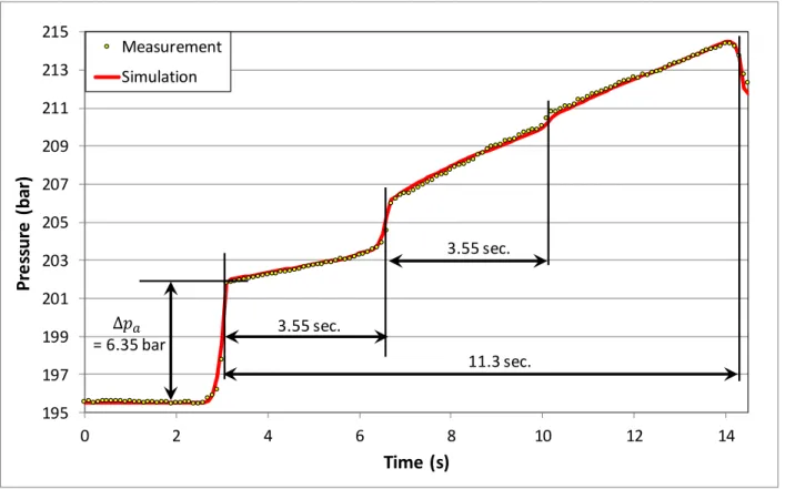
The test results show clearly the water hammer pressure (∆𝑝𝑎), and the reflection of the pressure pulse from the location of the tubing diameter change and from the bottom hole (see Figure 7). The pressure measurement has been performed at much higher frequency, however the data presented in the figure is down-sampled to 10 Hz. The first reflection that appears 3.55 seconds later after the water hammer effect is from the diameter change. This reflection repeats once more (attenuating as well); then the reflection from the bottom hole comes at 11.30 seconds. The reflection times provide the average speed of sound for the upper section of the tubing string (943 m/s) and for the whole wellbore (surface to bottom) as 973 m/s. Having calculated the average speed of sounds and considering the calculated values as the speed of sound values at the mean distance of each section, we can obtain the acoustic velocity profile: 930 m/s at the surface and 1016 m/s at the bottom (as a linear profile).

The density of oil is estimated by a PVT correlation as 710 kg/m3 _{at the wellhead flowing condition} (195 bar, 100°C) and 695 kg/m3 _{at the bottom hole flowing condition (approximately 590 bar, 170°C). The} oil density profile along the wellbore is considered as a linear variation of the distance from the wellhead.

Figure 7. Measured and simulated pressure pulse response at the wellhead

The magnitude of the water hammer pressure is the function of the in-situ acoustic velocity 𝑐, the density of flowing fluid 𝜌, and the fluid flowing velocity 𝑣 as stated by the Joukowsky equation:

∆𝑝_𝑎= 𝜌𝑣𝑐 (13)

Since the mass flow rate 𝑚 in a pipe with a constant cross-sectional area 𝐴 is 𝜌𝑣𝐴 it can also be found directly from the following relationship utilizing the Joukowsky equation:

𝑚 = ∆𝑝𝑎 𝐴

𝑐 (14)

provided that the speed of sound,𝑐 and the water-hammer pressure, ∆𝑝𝑎 are obtained from measurements.

The inside diameter of the surface tubing (3½ in. OD) is 74.2 mm. The water hammer pressure is measured as 6.35 bar (see Figure 7). The speed of sound at the surface is estimated as 930 m/s. Therefore,

195 197 199 201 203 205 207 209 211 213 215 0 2 4 6 8 10 12 14

P

re

ss

u

re

(

b

ar

)

Time (s)

the mass rate before the valve closure (which is used as the initial flow rate in the simulations) is calculated as 2.95 kg/s from Eq. 14.

The transient fluid flow model is used to simulate the case for which the input data are described above. Due to deposition on pipe walls, the flow diameter and the friction factor are the parameters to be adjusted to match the simulation results to the wellhead pressure measurement.

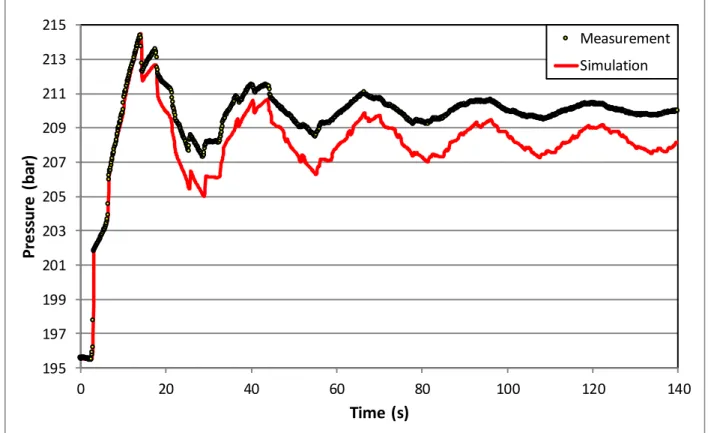
In addition, in order to have a well-posed problem a proper boundary condition at the bottom hole has to be applied. For the matching study to estimate deposition, we applied the constant bottom hole pressure boundary condition. We successfully matched the simulation results to the measurements as seen in Figure 7 by introducing a deposition of 1 mm in average along the upper section of the lower tubing string. However, the match was only for couple of seconds (or reflections); afterwards the deviation starts when the simulation runs for a long time (see Figure 8).

Figure 8. Measured and simulated pressure pulse response at the wellhead (simulation is performed

using the constant bottom hole boundary condition)

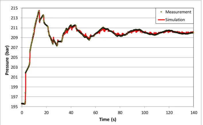
The pressure pulse data is history-matched by changing iteratively the transmissivity and the storativity until the discrepancy becomes sufficiently small. In other words, when the reservoir model with appropriate values of transmissivity and storativity is used as the bottom hole boundary condition, a good match is obtained for overall simulation time. Figure 9 presents the match, which was obtained with the transmissivity of 25 Darcy-m/cp and the storativity of 4.3 10-4 _{m/bar. Although we are not able} to compare these values with field data, the storativity value is a reasonable number, and the transmissivity is in the very acceptable range for carbonate rocks with fractures.

195 197 199 201 203 205 207 209 211 213 215 0 20 40 60 80 100 120 140

P

re

ss

u

re

(

b

ar

)

Time (s)

Figure 9. Measured and simulated pressure pulse response at the wellhead (simulation is performed

using the reservoir model as the bottom hole boundary condition)

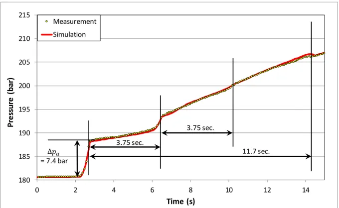
In the frame of testing campaign, another pressure pulse test has been also performed before the cleanup operation. The second set of field data is from this case. Although it is shorter, it can be still analyzed for the same purpose with the same approach explained earlier (see Figure 10). The first reflection, which is from the diameter change, appears 3.75 seconds after the hammer effect, though the reflection from the bottom hole comes at 11.70 seconds. Using those reflections, we obtain the acoustic velocities as 873 m/s at the surface and 1008 m/s at the bottom with linear variation assumption. The densities at the surface and the bottom hole are calculated as 709 and 695 kg/m3 _{respectively. The water} hammer pressure is measured as 7.4 bar. The mass rate is calculated 3.66 from Eq. 14. In order to match the simulation results to the measured data we slightly adjusted the mass rate (3.62 kg/s) and introduced a deposition of 4 to 5 mm in almost whole lower tubing string. We obtained a successful match as seen in Figure 10. 195 197 199 201 203 205 207 209 211 213 215 0 20 40 60 80 100 120 140

P

re

ss

u

re

(

b

ar

)

Time (s)

Figure 10. Measured and simulated pressure pulse response at the wellhead (before cleanup operation)

Figure 11. Comparison of simulated pressure pulse responses at the wellhead using the reservoir model

and the constant pressure boundary conditions with the measured data

As we have seen in the previous case, when the constant pressure boundary condition is used, we obtain a good match only for the first reflections. Then the simulation results deviate from the measurements (see the blue line in Figure 11).

180 185 190 195 200 205 210 215 0 2 4 6 8 10 12 14

P

re

ss

u

re

(

b

ar

)

Time (s)

The pressure pulse test before the cleanup operation has been performed at a higher flow rate and reduced diameter (due to deposition), which induces more frictional pressure drop. Although this test has obvious different flow condition than the one observed in the previous analysis, we still obtain a good match when the reservoir is modelled with very similar transmissivity and storativity values, i.e. T=23 Darcy-m/cp and S=4.0 10-4 _{m/bar. This suggests confirmation for reservoir parameters estimation} by matching analysis, though we are not able to compare the values with field data.

CONCLUSIONS

Transient pipe flow model was developed to be coupled to an analytical transient reservoir model. The transient pipe flow model solves the partial differential equations describing propagation of pressure pulse by a hyperbolic equation solver.

The transient analytical reservoir model is an analytical solution to the general diffusivity equation, which applies the principle of superposition in time to the line source solution of the diffusivity equation.

The coupled models were used to analyze field data from a single-phase oil well. The field data consists of rapid pressure measurements at the wellhead due to valve closure.

History matching approach is used to match the simulated pressure history to the measured pressure data at the wellhead. The reservoir parameters transmissivity and storativity in the near wellbore region were obtained from the history matching analysis.

Matching analysis of two sets of test data from different flowing conditions resulted in the same reservoir parameters.

ACKNOWLEDMENTS

The authors wish to acknowledge the support of this work by Markland Technology AS and by Eni, for having sponsored the project “Study of Monitoring and Removal of Deposits in Wells” in which the field data have been acquired. The project was possible also thanks to the contribution of Eni colleagues Vittorio Rota, Gilberto Toffolo and Martin Bartosek.

REFERENCES

Carey, M. A., Mondal, S., and Sharma, M. M., 2015. Analysis of Water Hammer Signatures for Fracture Diagnostics, SPE Paper 174866 presented the SPE Annual Technical Conference and Exhibition held in Houston, Texas, USA, 28–30 September 2015.

Chevray, R. and Mathieu, J., 1993. Topics in Fluid Mechanics, Cambridge University Press.

Chierici, G. L., 1994. Principles of Petroleum Reservoir Engineering Volume 1, Springer-Verlag Berlin. Falk, K. 1999. Pressure pulse propagation in gas-liquid pipe flow: modeling, experiments, and field

testing, Ph.D. dissertation, NTNU, Trondheim.

Horne, R.N., 1995. Modern Well Test Analysis, A Computer Aided Approach, 2nd edition, Petroway Inc., USA.

Howe, M. S., 2006. Hydrodynamics and Sound, Cambridge University Press.

Ghidaoui, M. S., Zhao, M., McInnis D. A., and Axworthy, D. H., 2005. A Review of Water Hammer Theory and Practice. Applied Mechanics Reviews 58(1), 49-76.

Gudmundsson, J. S. and Celius, H. K., 1999. Gas-Liquid Metering Using Pressure-Pulse Technology. SPE Paper 56584, Annual Technical Conference and Exhibiton, Houston, 3-6 October 1999.

Gudmundsson, J. S., Durgut, I., Celius, H. K. and Korsan, K., 2001. Detection and Monitoring of Deposits in Multiphase Flow Pipelines Using Pressure Pulse Technology. 12th International Oil Field Chemistry Symposium, Geilo, 1-4 April 2001.

Livescu, S., Watkins, T. J, 2014. Water Hammer Modeling in Extended Reach Wells. Paper SPE 168297 presented SPE/ICoTA Coiled Tubing & Well Intervention Conference and Exhibition, The Woodlands, TX, USA, 25-26 March 2014.

Mambretti, S., 2014. Water Hammer Simulations. WIT Press, Southampton, Boston.

Prümmer, R. 2009. History of Shock Waves, Explosions and Impact – A Chronological and Biographical Reference, Peter O. K. Krehl. Propellants, Explosives, Pyrotechnics, 34: 458.

Santarelli, F.J., Skomedal, E., Markestad, P., Berge, H.I., Nasvig, H., 2000. Sand Production on Water Injectors: Just How Bad Can It Get? SPE Drill. & Compl 15(2): 132.

Vaziri, H., Nouri, A., Hovem, K., Wang, X., 2007. Computation of Sand Production in Water Injectors. Paper SPE 107695 presented at the European Formation Damage Conference, Scheveningen, 30 May-1 June 2007.

Wang, X., Hovem, K., 2008. Water Hammer Effects on Water Injection Well Performance and Longevity. Paper SPE 112282 presented at the SPE International Symposium and Exhibition on Formation Damage Control, Lafayette, 13-15 February 2008.

Zazovsky, A., Tetenov, E. V., Zaki, K. S. and Norman W. D., 2014. “Pressure Pulse Generated by Valve Closure: Can It Cause Damage?” Paper SPE 168191 presented at SPE International Symposium and Exhibition on Formation Damage Control held in Lafayette, Louisiana, USA, 26–28 February 2014.

NOMENCLATURE

𝐴 Cross-sectional flow area of pipe (m2_{) 𝑞 Volumetric sandface flow rate (m}3_/s) 𝑐 Speed of sound (m/s) 𝑟𝑤 Wellbore radius (m)

𝑐𝑡 Total rock compressibility (1/Pa) 𝑡 Time (s)

𝐷 Flow diameter (m) 𝑡 Time (s)

𝑓 Darcy-Weisbach friction factor 𝑇 Transmissivity (Darcy-m/Pa·s and m3_/Pa·s) 𝑔 Acceleration of gravity (m/s2_{) 𝑣 Cross-sectional average fluid flow velocity (m/s)} ℎ Reservoir thickness (m) 𝑥 Direction along the pipe (m)

𝑘 Permeability (Darcy and m2_{) 𝑧 Opposite direction of gravity (m)} 𝑚 Mass flow rate(kg/s) 𝜇 Viscosity of fluid (cp and Pa·s) 𝑆 Storativity (m/Pa) 𝜙 Porosity (fraction)